
New Product Launching with Pricing, Free Replacement, Rework, and Warranty Policies via Genetic Algorithmic Approach
- DOI
- 10.2991/ijcis.d.190401.001How to use a DOI?
- Keywords
- New product launching; Price and warranty; Production; Genetic algorithm
- Abstract
New products are appearing in the marketplace at an ever-increasing step. Their launching is either market driven, or technology driven. Pricing and warranty policies play a vital role in launching of a new product, consequently growth of a company. In this paper a decision model is proposed to determine the pricing and warranty polices of a newly launched product considering free replacement during warranty period, and reworking during production process. We have assumed that the reworking is performed for the defective items, which are produced when a machine shifts from in-control state to out-of-control state to make them perfect. Profit function is formulated by combining the diffusion models and cost model. Structured optimal policies are proposed using optimal control theory and genetic algorithm solution approach is employed to explore the optimum values of price and warranty for every period of the product’s life cycle. Numerical example is presented considering different values of model parameters. Further, sensitivity analysis is performed to study the impact of model parameters on the profit model. The results of the paper will be greatly useful for the decision-makers, as it allows them to identify the role of the selected parameters during the entire life cycle of the product, and to study the long-term policy of a newly launched product.
- Copyright
- © 2019 The Authors. Published by Atlantis Press SARL.
- Open Access
- This is an open access article distributed under the CC BY-NC 4.0 license (http://creativecommons.org/licenses/by-nc/4.0/).
1. INTRODUCTION
Timely launch of a new product in market is becoming a necessary requirement for gaining a competitive advantage. In today’s scenario, a lot of pressure is faced by product development managers in launching a new product to market in record time. The various reasons for before-mentioned pressure are shorter product life cycles, growth of technological development, better mass communication, fragmentation of the marketplace due to the change in demographics, intense competition due to the maturing of markets and globalization, and the increasing cost of Research & Development (Ali et al., [1]). To survive in the market, a company must skillfully strategize product development process, its application, and management. Production process and sales are two major stages, which impact heavily on the entire life of product, even for survival and growth of the product as well as on the profitability of the company.
Generally, a production process is assumed to be perfect. But practically, when the demand of the product becomes high, the production system goes through a long-run process, that may transfer the manufacturing system from in-control to out-of-control state. As a result, two quality items are produced by this system-perfect and imperfect (defective). A cost is allowed to make the imperfect items as new as the perfect one. Also, companies set competitive price and offer warranty to boost the sales of the product. With consideration to the above facts, a production-sales profit maximization model to find the optimum level of price and warranty for a newly launched product considering production activities such as production, reworking of the imperfect items during production process is proposed. A warranty can be viewed as an indicator that delivers information about quality of the product and it also serves as an important marketing tool. Further, optimal control theory and genetic algorithm (GA) are applied for determining the optimum solution for the variables, that is, price and warranty under limited growth demand. The structure of this paper is as follows: Section 2 presents a brief literature review on marketing and/or technical strategy decisions, pricing and/or warranty, and imperfect production process. Problem definition, notations, and assumptions are provided in Section 3. The detailed formulation of demand/sale function, cost function, the production function along with model diagram, and the profit model is discussed in Section 4. The solution approach for the proposed model is discussed in Section 5. Numerical analysis of the model and sensitivity analysis is performed in Section 6. Finally, the conclusion is drawn in Section 7.
2. LITERATURE REVIEW
Launching a new product is a costly business. The role of the launch stage is to maximize the chance that a product profitably achieves an acceptance in the target market. Strategic and tactical launch decisions are the two main categories for a launch plan (Hultink et al., [2]). Strategic launch decisions include the product strategy, that is, the type of new product to be developed, market strategy, that is, the nature of the market into which the new product will be launched, competitive stance, and the firm’s overall orientation toward firm strategy. With reference to Tactical launch decisions it is well known that it targets the marketing aspects of the actual commercialization of the new product including the elements of the marketing mix along with the level of marketing investments, the breadth of product versions launched, how and where to distribute and promote the new product, and its price (Hultink et al., [2]). Although a majority of research from which we can derive normative guidelines for launching new products explored industrial markets (Montoya-Weiss and Calantone [3]), little empirical evidence is available regarding the launch decisions which are significant to the success of new products. Factors, which influence the launching decision of a product has been shown in Figure 1.
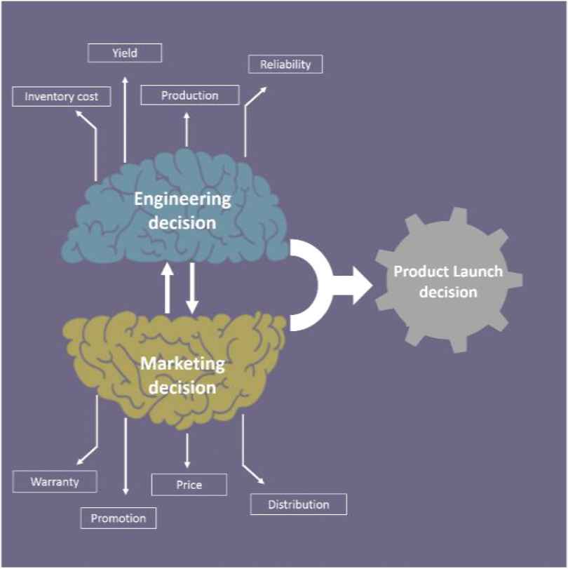
Factors influencing product launch decision.
The launching price is an integral part of the entire process. The pricing decisions are based on the launch price and the choice between skimming and penetration. High-priced product may yield more per unit profit but at the same time, it may result in decreased sales. For non-Giffen goods category, sales decreases as price increases, consequently, profit decreases (Lin and Shue [4]). Price also influence the production cost (incurred) because higher sales volume resulting from lower price may decrease the unit production cost. Also, a low-priced product attracts new buyers, who will remain loyal to the product in future, thus escalating profit. Therefore, to attract customers, manufacturers must set a competitive price that motivates the consumers to purchase the product. In general, price also serves as an evaluating tool of the product. Customers consider price as a major tool which influence their perspective toward a product, even if they lack complete information about the product (Suri and Monroe [5]).
Customers apply warranty information to review a product and to decide whether the price of the product is appropriate or not? Companies also apply warranty as a tool to judge the worth of product which improves the sales and increases the profit (Chien and Chen [6]; Ladany and Shore [7]). Short-term warranty does not convince customers enough about quality of product. But on the other hand, providing long-term warranty may result in very high cost of the product, also long-term warranty strategy has attracted manufacturers too (Chattopadhyay and Rahman [8]). Basically, the warranty length for a product is determined by the cost of warranty, which involves numerous factors like type of warranty, service mechanism of warranty, product failure rate, and the price (Rahman and Chattopadhyay [9]). From customer’s point of view, warranty is a fixed time commitment from the manufacturer, holding them responsible for any malfunctioning of product.
Various types of warranties are offered by the manufactures, some offer only repair, some offer restricted replacement with total repair, and some even offer total replacement. Actually, the fixed time length warranty is more acceptable form of warranty, where the warranty length of the renewed product is equal to the difference between length of the initial warranty and the period of usage of the faulty product being renewed. The warranty period is completed as soon as the complete life of product (initially purchased and subsequently renewed) has lasted the warranty length from the date of purchase. The renewals don’t affect the warranty period which still run from the initial point of purchase. Also, more warranty and less price increases the demand of product in the market.
In the past, researchers Lin and Shue [4] and Lin et al. [10] have done pioneer work for determining optimal pricing and warranty length of a product. Adida and Perakis [11] suggested a model based on demand in which they have assumed that demand is a linear function of the price, linear inventory cost, and the production cost, where cost of production is an increasing, strictly convex function of the production rate with all time-dependent coefficients. Glickman and Berger [12] in their work considered both price and warranty as the decision variables simultaneously with the objective to maximizing the profit. In their model, the authors guarantee repair of defective products, with the assumption that failures process is stochastic in nature while the cost for repair of defective product is constant. Teng and Thompson [13] proposed a model to maximize profit of a monopolist by determining optimal pricing and quality strategies. DiMicco et al. [14] and Raman and Chatterjee [15] suggested that manufacturers have the prospective to boost their income by selling the goods at customized price to buyers when the price is dynamic in nature. Wu et al. [16] proposed a model to maximize the profit by determining the optimal price and warranty-length strategies for a product with normal lifetime distribution. Later, Faridimehr and Niaki [17] wrote an erratum for the work proposed by Wu et al. [16]. Faridimehr and Niaki [18] investigated the optimal strategies for price, warranty length, and production rate of a new product considering static market for nondurable products and dynamic market for durable products.
The success of a new product depends on engineering decisions such as product reliability as well as marketing decisions, that is, its price, warranty (Huang et al. [19]). Even though a higher product reliability results in a higher manufacturing cost as well as an increase the sales price, consumers are still willing to pay more if an assurance about its reliability. Product warranty is one such indicator of reliability wherein longer warranty periods indicating better reliability (Istiana et al [20]). As warranty terms improve the sales of the product increases and drives expected warranty servicing costs higher. Thus, due to the learning effects on this cycle the unit manufacturing cost decreasing with total sales volume and this in turn impacts the sale price over time. This is the reason why price and warranty decisions need to be considered jointly. On the other hand, due to a long-run production process, machinery problems, labor problems, and so on, there is always a possibility of production of imperfect quality items. Companies rework on the defective items and make them perfect by adding a defective cost. Sarkar and Moon [21] proposed an Economic Production Quantity model incorporating the concept of inflation considering imperfect production system. Sarkar et al. [22] proposed a model to determine the optimum reliability of the product and production rate with the objective to maximize total profit for an imperfect manufacturing process. Sarkar et al. [22] used Euler–Lagrange theory to derive the necessary and sufficient conditions for optimality of the dynamic variables. Recently, Kumar et al. [23] proposed a model for determining optimal pricing policies of the product under the influence of reworking during production. Over a long survey of the literature and to the best of our knowledge, no effort has been made to develop the joint production-sales model which incorporates activities such as production, reworking of the imperfect items, and warranty during sale for a newly launched product. Keeping in mind the importance of these points, we have proposed a model to determine the optimal price and warranty strategy that achieves the maximum integrated profit for a general product sold under a free replacement warranty while also reworking during the imperfect production process. A key difference between the present study and the existing papers has been summarized in Table 1.
| Pricing Strategy | Warranty Strategy | Imperfect Production Process | Price, Warranty, and Cumulative Sales–Dependent Demand Function | GA Approach | Inventory Holding Cost Included | |
|---|---|---|---|---|---|---|
| Present model | Yes | Yes | Yes | Yes | Yes | Yes |
| Sarkar and Moon [21] | Yes | No | Yes | No | No | Yes |
| Research on pricing and warranty policies* | Yes | Yes | No | Yes | No | No |
| Lin et al. [10] | Yes | Yes | No | Yes | No | Yes |
GA, genetic algorithm.
Comparison between present research and prior research.
3. PROBLEM DEFINITIONS, NOTATION, AND ASSUMPTIONS
This section considers problem definition, notation, and the assumptions.
3.1. Problem Definitions
Our aim is to build a simple structured profit maximization model which integrates production process and sales. During production process, the concept of reworking of defective items is incorporated. These defective items are reworked at a cost to make the products as new as perfect one. We have also used a policy of free replacement of the faulty product during the warranty period. The cost associated with this type of warranty is equal to the cost of production, as the consumers receive a new product. The purpose of this is to find the profit function where price and warranty are the decision variables, which have to be optimized by using optimal control theoretic approach and GA approach.
The following notations and assumptions have been used to develop the model:
3.2. Notation
Q (t)–Cumulative production at time “t”
q (t)–Production rate at time “t”
S (t)–Sales at time “t”
p (t)–Selling price per unit item sold at time “t” (decision variable)
w (t)–Warranty period for products sold at time t (decision variable)
k1–Amplitude factor and k1 > 0
k2–Constant of time displacement and k2 > 0
α–Productivity factor, α > 1
β–Production amplitude factor, 0 < β < 1
co–Fixed cost of the products
γ–The learning rate, and 0 < γ < 1
f (p, w, S)–Sales rate at time “t” which is a function of price, warranty length, and sales
c (t)–Unit production cost which is a function of Q (t) at time “t”
c1–Per unit cost of reworking items for the time during which the production goes in-control state to out-of-control state
ch–Per unit inventory holding cost at a time “t”
M1 (t)–Excepted number of faulty items produced by the system at time “t” during the production process when the production is transfer from in-control state to out-of-control state with the assumptions that the faulty product follows exponentially distribution described in Appendix
M2 (w(t))–Expected number of renewals during the warranty length w (t).
TM2 (w(t))–Length of period
3.3. Assumptions
The production process is imperfect in nature and the model is developed for a single item.
During production process, perfect and imperfect item are produced, the perfect quality items are ready for sale and reworking is done for the imperfect items to make them perfect.
The discount rate is zero. Although, this assumption might seem unreasonable, it can be an approximation in markets with a very low discount rate. This shows that there is no difference between present and future profit in long-term horizon.
Time horizon is finite.
4. MATHEMATICAL MODELING
4.1. Sales Model
The sales of any product depend on several factors, such as price, warranty, advertising, competitive environment, and so on. Numerous mathematical models have been proposed earlier to examine the sales behavior of a product. Customers frequently use warranty and price information to assess the quality of a product and to decide if the product is suitable for buying. Thus, price and warranty are the two key deciding factors for the sales of a product. Glickman and Berger [12] suggested a demand function in which the demand decreases exponentially when the price increases whereas demand increases exponentially when warranty increases. Glickman and Berger [12] considered both price and warranty length as the decision variables, which are to be determined with the objective to maximize the overall profit. Longer warranty is a signal of more reliable product. This assumption can be justified by a number of empirical studies. For example, Wiener [28] proposed that in the markets for appliances and motor vehicles, warranties are exact signals of product reliability. Douglas et al. [29] found that in the US automobile market, a more intensive warranty is associated with higher-quality product. The demand function used in this paper is a limited growth demand function with the assumption that the demand function is a multiplicatively separable function of price and warranty and cumulative sales. Researchers, Clarke et al. [24], Kalish [25], Dockner and Jørgensen [26], Teng and Thompson [13], and Jørgensen et al. [27] used multiplicatively separable demand which is a function of price, warranty, and cumulative sales. This form of sales function is now widely acceptable in literature. Therefore, in line with Lin et al. [10], the demand/sales function is
4.2. Production Model
We have assumed that production depends on sales. The sales-dependent production function helps to optimize the production and inventory holding cost of the product. Another benefit of sales-dependent production function is that the resources are utilized in an optimal manner and produced relatively stable picture of the system that supports the future benefit. The mathematical form of the production function used in this paper is given by
As discussed by Wu et al. [16], the cost of producing a unit is defined as
Free renewal warranty policy is used to describe the warranty, in which the items are replaced free of cost during the warranty period with the assumption that the expected number of replacement during the warranty length w(t) is exponentially distributed (please refer to Appendix A). Mamer [30] explained different types of warranty policies and stated that the free renewal warranty policy is one of the most extensively policy used to cover consumer durables. Moreover, by using warranty associated cost, the cost function more becomes dynamic. The price of the product will increase if more products are replaced during the warranty period and it will decrease if fewer products are replaced. Figure 2 depicts the life cycle of product.
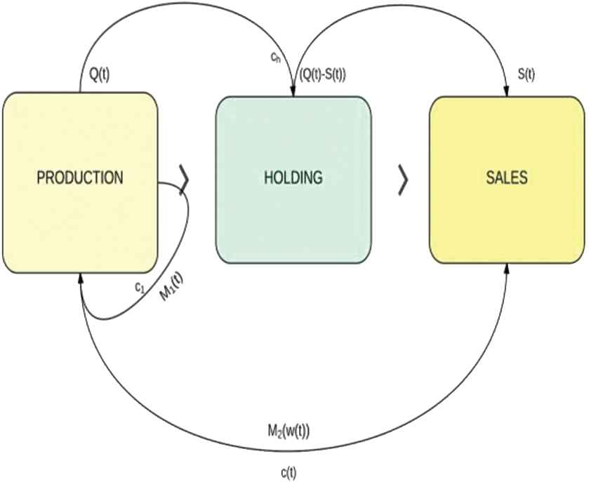
Model diagram of the product life.
4.3. Profit Maximization Model
With the above all considerations the profit maximization model is formulated as follows:
5. SOLUTION APPROACH
The above optimization model Equations (4–7) is solved by maximum principle. The Hamiltonian for the above optimization model is defined as follows (Sethi and Thompson [31]; Kapur et al. [32]; Kumar and Sahni [33]):
And the Lagrange’s function is,
The first order conditions are
Lp and Lw are the first order partial derivatives of L(t) with respect to price and warranty. According to Taylor’s theorem:
5.1. Genetic Algorithm (GA for Determining the Optimal Solution
In this section, we have described GA approach to obtain the best values of the decision variable, that is, price and warranty which also satisfy the objective function. GA is generally used when the optimal solution of problem is tough to find by classical optimization techniques. It is a random search base algorithm (Goldberg [34]), which follows the laws of natural selection, genetic information, and recombination with the population. It consists of operations: coding, calculating fitness, reproduction, crossover and mutation, appropriate values of population size, the probability of cross over, and finally the probability of mutation. GA is population-based adaptive search technique and highly effective when the search space of the problem is very large. GA is one of the best problem-solving approaches among other metaheuristics when large-scale problems are considered (Soleimani et al. [35]; Kumar et al. [36,37]). Researchers (Gupta et al. [38], Pasandideh et al. [39], Yang et al. [40]) applied GA to inventory management- related problems successfully. Kannan et al. [41] proposed a GA to minimize the total cost for a mixed-integer linear programming model with multi-echelon, multi-period, multi-product closed-loop supply chain network containing storage space and processing time restrictions. Pasandideh et al. [42] developed a random demand and limited storage capacity multi-period multi-item inventory control problem with the objective to determine the optimal order quantities of products in different periods and minimizing the total inventory cost. Saracoglu et al. [43] proposed an approach for multi-product multi-period (Q, r) inventory models to obtain the optimal order quantity and optimal reorder point under the constraints of shelf life, budget, storage capacity, and “extra number of products” promotions according to the ordered quantity. Saracoglu et al. [43] modeled the problem as an integer linear programming (ILP) model and then applied GA solution approach to solve larger scale problems.
Evolutionary computation methods are appropriate to solve complex and nonconvex bidding strategy problem. Therefore, in this paper, GA is used as an important evolutionary computation algorithm to solve this optimization problem. The proposed methodology consists of following components:
Population size: Here, the population corresponds to a sample of the complete solution set. Typically, the population size of a GA is a fraction of the whole solution set. The number of chromosomes in each generation will directly affect the time taken to find optimal solution to a given problem. If there are too few chromosomes, then there are few possibilities to carry out crossover and only a small part of the search space is explored. This may result in GA finish with a suboptimal solution. However, if there are too many chromosomes, GA will slow down, outweighing the attractiveness of this algorithm over the conventional solution techniques. Previous works have shown that populations with moderate-sized are best suited for many practical problems (Gupta et al. [38]; Yang et al. [40]).
Representation: The solution process begins with a set of identified chromosomes as the parents from a population.
Initialization: The population of chromosome is randomly initialized within the operating range of the control variables.
Reproduction: In a given generation the “Healthiest” chromosomes are used to form the chromosomes of the new population in the next generation and this new population is selected with the hope that it will be better than the old one. The members of the subsequent generation are called offspring. Competition method is used for chromosome selection in this approach. Selected chromosomes compose Mating pool. In fact, reproduction operator selects a set of the best chromosomes, but none of these are new and to tackle this Crossover operators are used to create new chromosome from randomly selected chromosome from mating pool. Here, offspring formulation will use heredity which is defined by two basic operations: mutation and crossover.
Crossover: The creation of offspring from its parents is done using the principles of crossover. In the process, some genes are selected from one subset of parents and mixed with different genes from other parents.
Mutation: Mutation process leads an offspring to have their own identity. Usually a very low mutation rate is selected to decrease the amount of randomness introduced in the solution. Selecting a proper level of mutation is the key to avoid a GA from getting captured in local minima.
Termination criteria: There are various methods to end GA running.
Figure 3 describes the flow chart to implement Genetic algorithm for our proposed model.
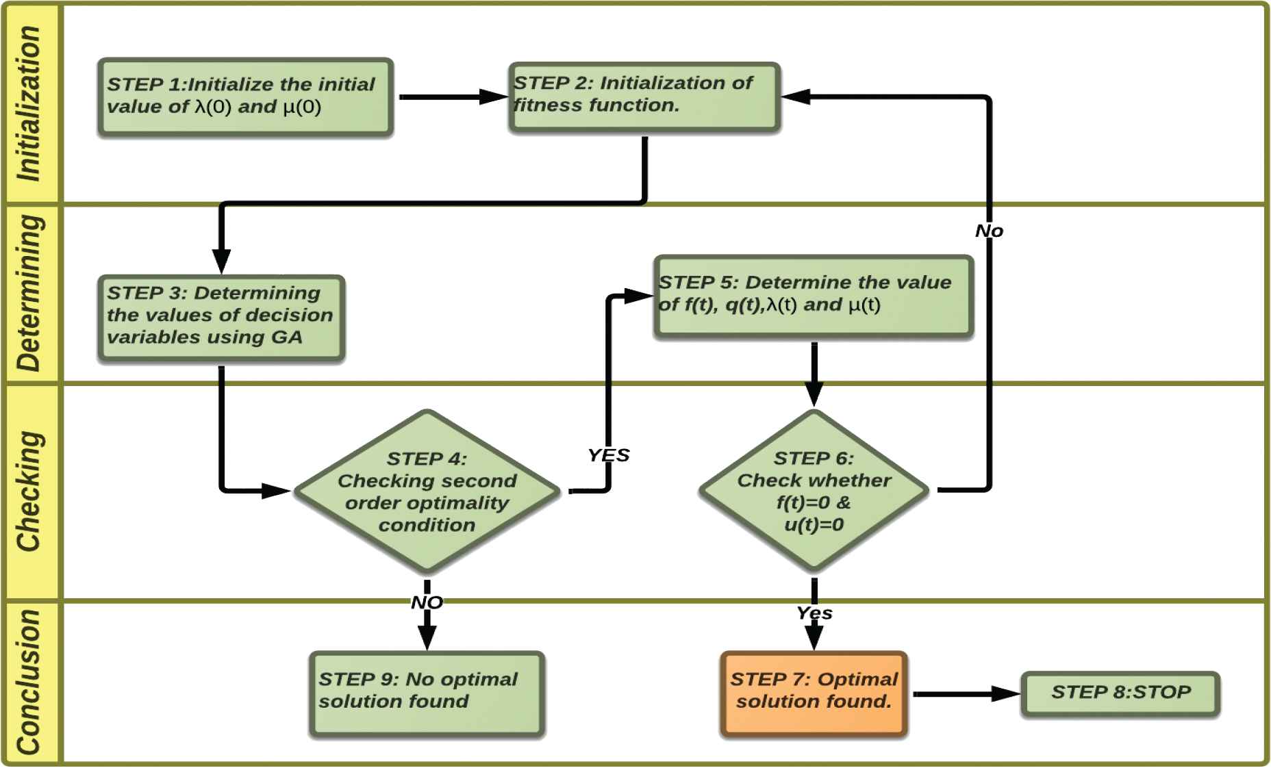
Flowchart of genetic algorithm (GA) for determining the optimal solution.
The fitness function to maximize the profit is given by:
To obtain the best optimum solutions for decision variables, that is, price and warranty, the second order optimality conditions are
Various parameter values considered for using GA are given below in Table 2.
| Parameters | Value |
|---|---|
| Population size | 1000 |
| Probability of mutation | 0.01 |
| Probability of crossover | 0.85 |
| Upper bound | 1500 |
| Difference between twoconsecutive iteration | 0.0001 |
Parameters for genetic algorithm.
6. NUMERICAL EXAMPLE
The numerical example is to test the applicability of the model. The solution was obtained using GA tool in MATLAB 7.11 software. Firstly, some base values are considered which are
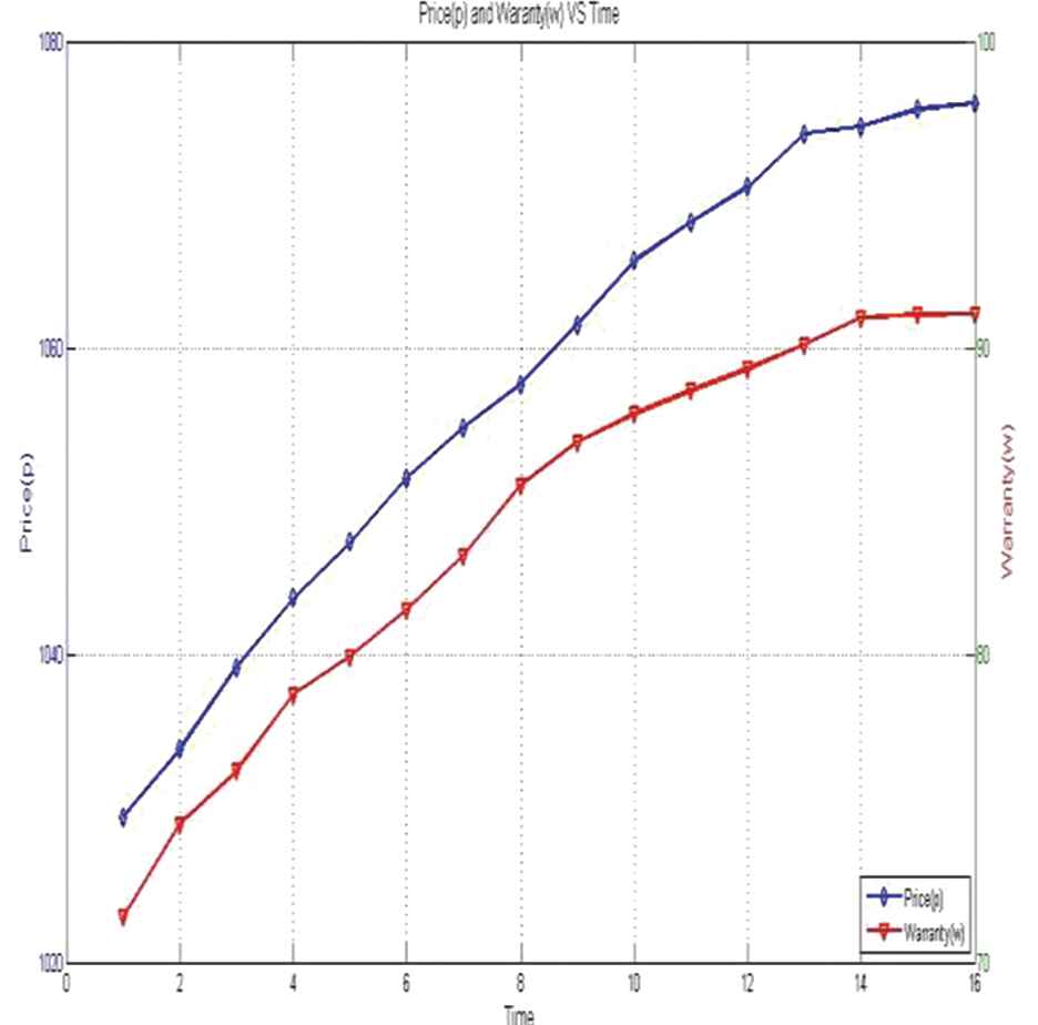
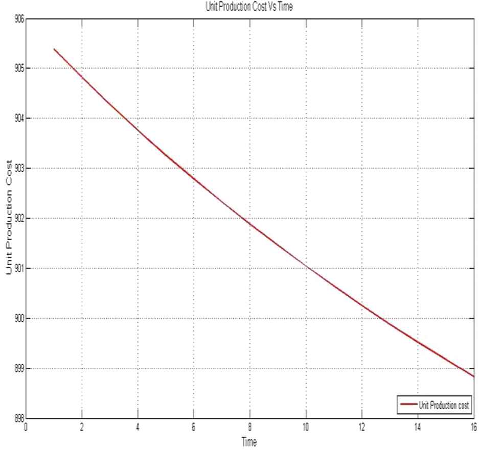
Table 3 describes the optimum values of price and warranty with the objective of maximum profit. Various model parameters are varied to perform the sensitivity analysis of the parameters. The model is solved on the basis of the first two values of λ (0) = 150 and λ (0) = 145 separately (keeping other parameters fixed) and observed that with the decrease in value of λ (0), the cumulative profit decreases. In addition to this, the warranty length of the product increases. Figure 4 depicts the optimal value of price and warranty with time. Variation in unit production cost with time is shown in Figure 5.
| t | Price (p(t)) | Warranty (w(t)) | Cumulative Sale (S(t)) | Unit Production Cost c(t) | Cumulative Profit |
|---|---|---|---|---|---|
| 1 | 1028.74 | 67.21 | 924.77 | 901.762656 | 425,680.21 |
| 2 | 1031.75 | 68.90 | 943.04 | 900.064255 | 500,420.17 |
| 3 | 1040.15 | 69.58 | 956.93 | 898.747577 | 687,430.99 |
| 4 | 1046.23 | 70.34 | 967.38 | 897.706446 | 740,460.91 |
| 5 | 1051.56 | 71.54 | 975.27 | 896.865934 | 794,601.76 |
| 6 | 1056.87 | 72.12 | 981.25 | 896.176804 | 806,820.14 |
| 7 | 1059.31 | 73.91 | 985.77 | 895.606516 | 809,407.51 |
| 8 | 1063.67 | 74.84 | 989.22 | 895.128583 | 796,803.25 |
| 9 | 1069.12 | 75.54 | 991.83 | 894.726820 | 778,168.68 |
| 10 | 1072.43 | 76.32 | 993.80 | 894.387555 | 753,923.29 |
| 11 | 1075.52 | 77.19 | 995.30 | 894.099322 | 727,188.92 |
| 12 | 1076.87 | 78.02 | 996.43 | 893.853472 | 698,880.79 |
| 13 | 1077.13 | 78.98 | 997.30 | 893.642984 | 670,155.89 |
| 14 | 1077.42 | 79.63 | 997.95 | 893.462227 | 641,541.46 |
| 15 | 1077.49 | 80.01 | 998.45 | 893.306845 | 613,498.46 |
| 16 | 1077.48 | 80.03 | 998.83 | 893.173131 | 586,254.17 |
Solution of original example when λ (0) = 150 and µ = 5.0.
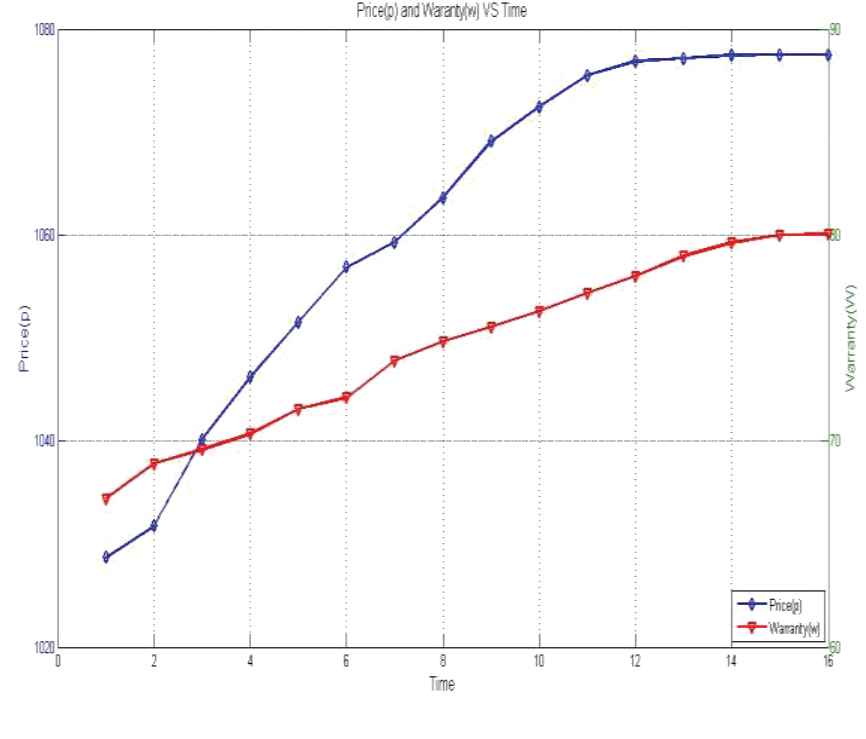
Graph depicting price and warranty with time “t” at λ (0) = 150.

Unit production cost with time “t” at λ (0) = 150.
Now changing the value of λ (0) = 150 to λ (0) = 145 and keeping other parameters same as in earlier case. The above procedure is repeated to determine its impact of λ on price, warranty, and other parameters. Table 4 shows the optimum values of price and warranty at any time point “t.” Figure 6 depicts the optimal value of price and warrant with time for λ (0) = 145 and the variation in unit production cost with time is shown in Figure 7.
| t | Price (p(t)) | Warranty (w(t)) | Cumulative Sale (S(t)) | Unit Production Cost c(t) | Cumulative Profit |
|---|---|---|---|---|---|
| 1 | 1029.482 | 71.472 | 924.77 | 901.762656 | 2,703,904.44 |
| 2 | 1033.896 | 74.498 | 943.36 | 900.050134 | 1,781,217.27 |
| 3 | 1039.236 | 76.237 | 957.47 | 898.725111 | 2,410,006.69 |
| 4 | 1043.732 | 78.721 | 968.08 | 897.677906 | 2,271,427.57 |
| 5 | 1047.391 | 79.971 | 976.09 | 896.833375 | 2,407,715.89 |
| 6 | 1051.541 | 81.482 | 982.09 | 896.144686 | 2,383,413.56 |
| 7 | 1054.833 | 83.242 | 986.59 | 895.576962 | 2,399,540.44 |
| 8 | 1057.639 | 85.532 | 989.98 | 895.104699 | 2,379,160.25 |
| 9 | 1061.537 | 86.961 | 992.52 | 894.708958 | 2,361,859.98 |
| 10 | 1065.688 | 87.873 | 994.42 | 894.376525 | 2,335,508.12 |
| 11 | 1068.214 | 88.632 | 995.83 | 894.096346 | 2,308,495.21 |
| 12 | 1070.542 | 89.342 | 996.89 | 893.859158 | 2,279,572.89 |
| 13 | 1073.985 | 90.123 | 997.68 | 893.657743 | 2,250,791.36 |
| 14 | 1074.432 | 91.002 | 998.27 | 893.486340 | 2,222,279.69 |
| 15 | 1075.542 | 91.087 | 998.71 | 893.339905 | 2,194,573.90 |
| 16 | 1075.983 | 91.112 | 999.04 | 893.214832 | 2,167,818.77 |
Solution of the model when λ (0) = 145 and µ = 5.0.
Price and warranty with time “t” at λ (0) = 145.
Unit production cost with time “t” at λ (0) = 145.
6.1. Sensitivity Analysis
In the above model the optimal solution depends on the various parameters which are the key parameters of the objective function and the values of these parameters affect the solution. The sensitivity analysis helps to determine the impact of the various parameters on the solution of the model. To perform the sensitivity analysis on the proposed model, the value of coefficient of price (a) is varied from 1.05 to 1.20 and its impact on the price, warranty, and cumulative profit is observed thoroughly. Similarly the effect of other parameters, that is, coefficient of warranty (b), total factor productivity (α), and learning rate (β) on the profit maximization model were analyzed. This will help to make the decision model closer to real-world situation.
6.1.1. Effect of change in coefficient of price (a)
When the values of the coefficient of the price is set from 1.05 to 1.15, the increase in the value of a, cumulative sales of the product decreases which results in decline of the cumulative profit. The effect for the different values is analyzed on model components and is tabulated below. Table 5 depicts all the above possible cases. From the Tables 5(a) and 5(b), when the price is 1031.75 then the corresponding warranty is 68.90 weeks but when the value of a is increased with price of 1031.65 the company is offering the warranty of 66.23 weeks. Due to decrease in warranty with same price leads to the decrease in the cumulative sale and hence the profit is reduced. From Tables 5(b) and 5(c) in second row, price of the product is increases from 1039.01 to 1044.56 and at the same time the warranty length of the product decreases from 68.35 weeks to 66.98 weeks which affects the cumulative sale and hence the net profit is reduced.
| t | Price (p(t)) | Warranty (w(t)) | Cumulative Sale (S(t)) | Unit Production Cost c(t) | Cumulative Profit |
|---|---|---|---|---|---|
| (a) When α = 1.05 | |||||
| 1 | 1028.74 | 67.21 | 924.77 | 901.762656 | 425,680.21 |
| 2 | 1031.75 | 68.90 | 943.04 | 900.064255 | 500,420.17 |
| 3 | 1040.15 | 69.58 | 956.93 | 898.747577 | 687,430.99 |
| 4 | 1046.23 | 70.34 | 967.38 | 897.706446 | 740,460.91 |
| 5 | 1051.56 | 71.54 | 975.27 | 896.865934 | 794,601.76 |
| (b) α = 1.10 | |||||
| 1 | 1031.65 | 66.23 | 917.53 | 902.102543 | 226,462.84 |
| 2 | 1039.01 | 68.35 | 931.58 | 900.563209 | 266,367.84 |
| 3 | 1048.54 | 70.71 | 943.26 | 899.305150 | 413,690.30 |
| 4 | 1056.32 | 71.99 | 952.95 | 898.258153 | 458,224.51 |
| 5 | 1063.76 | 72.87 | 960.95 | 897.375316 | 514,965.42 |
| (c) α = 1.15 | |||||
| 1 | 1035.13 | 66.01 | 912.41 | 902.395681 | 89,493.29 |
| 2 | 1044.56 | 66.98 | 922.91 | 901.025159 | 102,181.90 |
| 3 | 1053.87 | 67.76 | 932.09 | 899.863901 | 205,943.50 |
| 4 | 1061.14 | 68.48 | 940.13 | 898.865615 | 233,486.50 |
| 5 | 1070.56 | 69.18 | 947.18 | 897.996400 | 278,662.21 |
Sensitivity results for (a) α = 1.05, (b) α = 1.10, (c) α = 1.15.
6.1.2. Effect of change in coefficient of warranty (b)
Table 6 depicts the variations in price and warranty when the coefficient of the warranty is set from 0.3 to 0.6, increase in the value of b the cumulative sale of the product increases which results in the rapid increase in the cumulative profit of the product. From the Tables 6(a) and 6(b), initially the price is 1028.74 and the corresponding warranty is 67.21 weeks but when the value of the b is increased from 0.3 to 0.4 the price decreased to 1024.48 and corresponding warranty increased to 68.65 weeks which helps to increase the cumulative sales and hence the profit is increased.
| t | Price (p(t)) | Warranty (w(t)) | Cumulative Sale (S(t)) | Unit Production Cost c(t) | Cumulative Profit |
|---|---|---|---|---|---|
| (a) b = 0.3 | |||||
| 1 | 1028.74 | 67.21 | 924.77 | 901.762656 | 425,680.21 |
| 2 | 1031.75 | 68.90 | 943.04 | 900.064255 | 500,420.17 |
| 3 | 1040.15 | 69.58 | 956.93 | 898.747577 | 687,430.99 |
| 4 | 1046.23 | 70.34 | 967.38 | 897.706446 | 740,460.91 |
| 5 | 1051.56 | 71.54 | 975.27 | 896.865934 | 794,601.76 |
| (b) b = 0.4 | |||||
| 1 | 1024.48 | 68.65 | 937.60 | 901.280994 | 788,473.69 |
| 2 | 1027.71 | 69.03 | 960.98 | 899.441178 | 907,763.05 |
| 3 | 1030.13 | 69.81 | 975.58 | 898.154058 | 1,107,086.94 |
| 4 | 1033.67 | 70.27 | 984.74 | 897.219688 | 1,144,449.65 |
| 5 | 1038.02 | 70.73 | 990.46 | 896.526974 | 1,167,533.49 |
| (c) b = 0.5 | |||||
| 1 | 1021.01 | 67.34 | 957.08 | 900.711440 | 1,351,949.47 |
| 2 | 1024.28 | 68.21 | 981.47 | 898.911060 | 1,480,136.55 |
| 3 | 1028.47 | 69.01 | 992.04 | 897.851445 | 1,604,151.80 |
| 4 | 1031.81 | 69.99 | 996.58 | 897.201173 | 1,595,579.44 |
| 5 | 1034.71 | 70.65 | 998.54 | 896.791848 | 1,576,917.96 |
| (d) b = 0.6 | |||||
| 1 | 1028.74 | 66.12 | 986.65 | 900.042881 | 2,223,938.43 |
| 2 | 1031.75 | 67.71 | 997.99 | 898.849117 | 2,240,437.51 |
| 3 | 1040.15 | 68.84 | 999.72 | 898.412413 | 2,226,497.03 |
| 4 | 1046.23 | 69.95 | 999.96 | 898.252266 | 2,205,965.55 |
| 5 | 1051.56 | 71.07 | 999.99 | 898.192862 | 2,193,368.63 |
Sensitivity results for (a) b = 0.3, (b) b = 0.4, (c) b = 0.5, (d) b = 0.6.
6.1.3. Effect of total factor productivity (α)
Table 7 depicts the variations in price and warranty with respect to α. A change in the value of α from 43 to 42, increases the price from 1031.75 to 1033.12 and decreases the corresponding warranty from 68.90 weeks to 67.67 weeks as shown in the second row of the Tables 7(a) and 7(b). This causes the cumulative sales of the product to increase and the unit production cost also increases negligibly. The slight increase in unit production cost reduces the cumulative profit. The last row of the Tables 7(c) and 7(d) depicts a different trend. By decreasing the value of α from 41 to 40, the price of the product is decreased, and warranty increases minimally. This causes the cumulative sales to decrease and unit production cost to decrease fractionally, consequently cumulative profit decreases. Thus, if the change in price and warranty is very less, cumulative profit of the model will increase but if the change is large the cumulative profit will decrease.
| t | Price (p(t)) | Warranty (w(t)) | Cumulative Sale (S(t)) | Unit Production Cost c(t) | Cumulative Profit |
|---|---|---|---|---|---|
| (a) α = 43 | |||||
| 1 | 1028.74 | 67.21 | 924.77 | 901.762656 | 440,432.04 |
| 2 | 1031.75 | 68.90 | 943.04 | 900.064255 | 515,172.00 |
| 3 | 1040.15 | 69.58 | 956.93 | 898.747577 | 702,182.82 |
| 4 | 1046.23 | 70.34 | 967.38 | 897.706446 | 755,212.74 |
| 5 | 1051.56 | 71.54 | 975.27 | 896.865934 | 809,353.59 |
| (b) α = 42 | |||||
| 1 | 1029.98 | 66.12 | 924.77 | 901.811932 | 440,496.86 |
| 2 | 1033.12 | 67.67 | 942.92 | 900.149374 | 514,832.61 |
| 3 | 1037.65 | 68.98 | 956.75 | 898.856605 | 701,870.19 |
| 4 | 1043.42 | 69.65 | 967.24 | 897.828333 | 755,058.18 |
| 5 | 1051.72 | 70.06 | 975.16 | 896.997479 | 810,160.72 |
| (c) α = 41 | |||||
| 1 | 1031.12 | 65.43 | 924.77 | 901.861398 | 440,559.18 |
| 2 | 1036.45 | 66.21 | 942.85 | 900.233397 | 514,698.79 |
| 3 | 1040.78 | 67.24 | 956.55 | 898.967162 | 701,480.94 |
| 4 | 1044.89 | 69.02 | 966.98 | 897.957091 | 754,161.98 |
| 5 | 1050.94 | 69.56 | 974.93 | 897.135926 | 810,225.03 |
| (d) α = 40 | |||||
| 1 | 1034.76 | 64.81 | 924.77 | 901.911056 | 440,683.37 |
| 2 | 1038.68 | 65.37 | 942.73 | 900.319489 | 514,400.12 |
| 3 | 1041.88 | 66.17 | 956.38 | 899.077102 | 701,254.64 |
| 4 | 1046.21 | 67.76 | 966.78 | 898.083454 | 753,950.10 |
| 5 | 1050.03 | 69.79 | 974.73 | 897.274355 | 810,708.13 |
Sensitivity results for (a) α = 43, (b) α = 42, (c) α = 41, (d) α = 40.
6.1.4. Effect of the learning rate (β)
Table 8 shows the impact of β on the profit maximization model. β is increased from 0.5 to 0.8 keeping the other parameters fixed. By increasing the value of β, the price of the product decreases and at the same time the warranty length increases, which results increase in the cumulative sales. Here, the cumulative profit decreases even after increase in the cumulative sales because the decrease in the price of the product is high as compared to cumulative sales and hence net profit decreases.
| t | Price (p(t)) | Warranty (w(t)) | Cumulative Sale (S(t)) | Unit Production Cost c(t) | Cumulative Profit |
|---|---|---|---|---|---|
| (a) β = 0.5 | |||||
| 1 | 1028.74 | 67.21 | 924.77 | 901.762656 | 440,432.04 |
| 2 | 1031.75 | 68.90 | 943.04 | 900.064255 | 515,172.00 |
| 3 | 1040.15 | 69.58 | 956.93 | 898.747577 | 702,182.82 |
| 4 | 1046.23 | 70.34 | 967.38 | 897.706446 | 755,212.74 |
| 5 | 1051.56 | 71.54 | 975.27 | 896.865934 | 809,353.59 |
| (b) β = 0.6 | |||||
| 1 | 1025.51 | 69.00 | 924.77 | 900.986368 | 439,791.94 |
| 2 | 1029.24 | 71.00 | 943.24 | 898.870541 | 514,000.05 |
| 3 | 1033.21 | 73.00 | 957.25 | 897.317787 | 699,141.52 |
| 4 | 1036.86 | 75.00 | 967.84 | 896.137682 | 750,821.42 |
| 5 | 1040.23 | 71.54 | 975.84 | 895.219117 | 801,955.53 |
| (c) β = 0.7 | |||||
| 1 | 1023.28 | 67.93 | 924.77 | 899.988125 | 438,950.89 |
| 2 | 1026.02 | 68.27 | 943.20 | 897.420543 | 510,819.11 |
| 3 | 1029.52 | 68.79 | 957.09 | 895.642176 | 693,495.28 |
| 4 | 1031.18 | 69.06 | 967.58 | 894.347906 | 741,399.55 |
| 5 | 1034.75 | 69.63 | 975.50 | 893.375141 | 790,080.79 |
| (d) β = 0.8 | |||||
| 1 | 1021.34 | 68.08 | 924.77 | 898.728675 | 437,797.42 |
| 2 | 1023.72 | 68.42 | 943.25 | 895.670779 | 507,067.97 |
| 3 | 1026.75 | 68.81 | 957.17 | 893.669170 | 686,601.51 |
| 4 | 1029.32 | 69.02 | 967.67 | 892.272345 | 730,816.97 |
| 5 | 1031.76 | 69.35 | 975.58 | 891.259192 | 775,183.08 |
Sensitivity results for (a) β = 0.5, (b) β = 0.6, (c) β = 0.7, (d) β = 0.8.
7. CONCLUSIONS
Technology development brings prosperity to nations, but the successful commercialization of the technology is the real meaning of innovation. For this reason, all companies have tried their best to launch maximum numbers of products to market. However, commercial success or failure of a product does not rest solely on the product itself. The launch strategy adopted also determines whether a product succeeds or fails. The key to success in the launch process often rests in finding the proper strategies. Previous studies have discussed a number of relevant issues, but few studies have addressed new product launch strategy planning. In this paper, we have made a first attempt to formulate the mathematical model for a new product launch strategy incorporating joint effect of its production and sales. The model involves optimally selecting the warranty period and the price to maximize the expected profit for a product sold with a free replacement policy during warranty period.
During production run-time, a certain percentage of total production is defective which is reworked to make them perfect. Optimal control theory is applied to find the theoretical aspect of the model while GA is applied to obtain the optimal values of price and warranty for the manufactures. Based on replacement policy, the total unit cost of product is determined and, on this basis, total profit is calculated. During the modeling, we have assumed that the production function is depended upon the demand. This assumption optimizes the production, the inventory holding cost, and resources. From the simulation, we observed that any increase in warranty length increases the price of product, but for the longer warranty, cost does not increase more rapidly. It is found that both price and warranty should be preset in the same direction to find the best optimum results. Moreover, at the same price, the warranty length can be changed, and consequently change in cumulative profit. By changing the various decision parameters, the cumulative profit also changes. By varying coefficient of price, the warranty length changes significantly. Due to which the cumulative profit of the product shows rapid decline. When the value of coefficient of warranty is increased, sales rate is also increased, and inventory is reduced. Therefore, increase in the sales rate reduced the price which helps to increase the cumulative profit.
The major contributions of this model are to approximate optimum value of price and warranty for a new product when free replacement during warranty and reworking is the part of business policy. Thus, it can be propagated that model has a new managerial insight which helps a manufacturing system/industry to gain the profit at optimal level for a newly launched product. Also, the manufactures must collect the relevant information of input parameters before implementing this model for obtaining the optimum value of price and warranty. The proposed model is best suited for products that hope to gain market share while offering medium to long-term warranty, for example, solar panels that offer free replacement warranties between 10 and 25 years which demonstrating its reliability to the customer. The model can also have applied travel goods such as suitcases and travel pack whose fundamental design has remained the same but their warranties and thoroughly tested products make them stand apart, for example, Samsonite’s 10-year Global warranty for some of its products.
The proposed model does not consider the product with short life cycle because there are great variations in price for short life cycle products, for example, many of the electronic parts that compose a product have a life cycle that is significantly shorter than the life cycle of the product. The part becomes obsolete when it is no longer manufactured, either because demand has dropped to low enough levels that it is no longer practical for manufacturers to continue to make it, or because the materials necessary to produce it are no longer available. Moreover, the public’s demand for products with increased warranties makes this problem only worse. Therefore, unless the system being designed has a short life (manufacturing and field), or the product is the driving force behind the part’s market (e.g., personnel computers driving the microprocessor market), there is a high likelihood of a life cycle mismatch between the parts and the product. The life cycle mismatch problem requires that during design, engineers take into account which parts will be available and which parts may be obsolete during a product’s manufacturing run, such design phase factors have not been included in this model. This problem is prevalent in many avionics and military systems, where systems may encounter obsolescence problems before being fielded and often experience obsolescence problems during field life. In future research, this model can further be generalized to include the nondeterministic demand function.
ACKNOWLEDGMENTS
Authors sincerely thank the reviewers for their valuable suggestions that have incorporated to enhance the quality of the work.
APPENDIX A EXPONENTIAL DISTRIBUTION
Let Y1, Y2, ………… Yn be nonnegative random variables, which are exponentially distributed with failure rate λ at any time, then the sum of n identically distributed random lifetimes is distributed as Gamma with shape parameter and scale parameter. Where,
Y1, Y2, ………… Yn are the lifetimes of successive items (independent and identically distributed)
Gn = the sum of n identically distributed random lifetimes.
The renewal function, its first and second derivative with respect to w are defined as
REFERENCES
Cite this article
TY  - JOUR
AU  - Vijay Kumar
AU  - Biswajit Sarkar
AU  - Alok Nath Sharma
AU  - Mandeep Mittal
PY  - 2019
DA  - 2019/01/31
TI  - New Product Launching with Pricing, Free Replacement, Rework, and Warranty Policies via Genetic Algorithmic Approach
JO  - International Journal of Computational Intelligence Systems
SP  - 519
EP  - 529
VL  - 12
IS  - 2
SN  - 1875-6883
UR  - https://doi.org/10.2991/ijcis.d.190401.001
DO  - 10.2991/ijcis.d.190401.001
ID  - Kumar2019
ER  -