
An Efficient Modified Particle Swarm Optimization Algorithm for Solving Mixed-Integer Nonlinear Programming Problems
- DOI
- 10.2991/ijcis.d.190402.001How to use a DOI?
- Keywords
- Particle swarm optimization; Mixed-integer nonlinear programming; Constrained optimization; Simulated annealing
- Abstract
This paper presents an efficient modified particle swarm optimization (EMPSO) algorithm for solving mixed-integer nonlinear programming problems. In the proposed algorithm, a new evolutionary strategies for the discrete variables is introduced, which can solve the problem that the evolutionary strategy of the classical particle swarm optimization algorithm is invalid for the discrete variables. An update strategy under the constraints is proposed to update the optimal position, which effectively utilizes the available information on infeasible solutions to guide particle search. In order to evaluate and analyze the performance of EMPSO, two hybrid particle swarm optimization algorithms with different strategies are also given. The simulation results indicate that, in terms of robustness and convergence speed, EMPSO is better than the other algorithms in solving 14 test problems. A new performance index (NPI) is introduced to fairly compare the other two algorithms, and in most cases the values of the NPI obtained by EMPSO were superior to the other algorithms.
- Copyright
- © 2019 The Authors. Published by Atlantis Press SARL.
- Open Access
- This is an open access article distributed under the CC BY-NC 4.0 license (http://creativecommons.org/licenses/by-nc/4.0/).
1. INTRODUCTION
In the fields of science and engineering, researchers have a great interest in solving optimization problems consisting of real and discrete (or integer) variables. These are called mixed-integer programming (MIP) problems, which arise from a variety of real-world situations and applications. For example, Alavidoost et al. [1] described a supply-chain network with an MIP problem and solved it by using a genetic algorithm. Willis et al. [2] used an MIP to search in the superstructure of chemical reaction networks. Cobuloglu et al. [3] presented a two-stage stochastic MIP model to maximize the economic and environmental benefits of food and biofuel production. Merchan et al. [4] studied discrete-time MIP models to solve the production scheduling problem. Ku et al. [5] used an MIP to solve job shop scheduling. Benati et al. [6] established an MIP model to solve the feature selection problem in clustering and a heuristic method was given. There are many other studies on MIPs [7–10].
An MIP problem is described as follows:
where x ∈ ℝl represents the continuous variables, y ∈ ℤm represents the discrete or integer variables, and
If any of f(x, y) or gi(x, y) are nonlinear functions, then the problem is called mixed-integer nonlinear programming (MINLP). When x ∈ {0, 1}, it is called 0–1 mixed-integer nonlinear programming (0–1 MINLP). If none of the decision variables are continuous variables, the problem is called integer programming (IP).
Both integer and MIP are Non-deterministic Polynomial-hard, and the difficulty to solve these problems increases exponentially with size [11]. The traditional optimization algorithms can only deal with simple optimization problems, and cannot be used to solve complex problems. Therefore, a large number of stochastic algorithms are proposed and applied to solve such problems.
Current studies on mixed-integer optimization problems typically focus on some special models, such as the convex model, 0–1 MIP, and so on. At present, research mainly concentrates on the following four approaches: (1) The integer continuity method [12]. In this approach, the continuous optimization algorithm is first used to calculate the optimal solution without integer constraints. Then, the integer variables are rounded into the feasible domain. So, the approximate optimal solution is found. This method can easily solve the continuous optimization problem; however, this has low precision in the process of converting continuous variables into integer variables, and perhaps may not find the optimal solution for some problems. (2) The deterministic method, which uses the branch boundary method [13] and the cutting-plane approach [14] to solve MIP problems. These methods are effective and efficient for solving small-scale problems but, when the scale of the problem increases and the degree of nonlinearity becomes higher, the deterministic method is usually incapable of solving the problem. (3) Monte Carlo methods [15] comprise a broad class of computational algorithms that rely on repeated random sampling to obtain an approximate solution of an MIP problem. From a theoretical point of view, a Monte Carlo method can find a better solution with enough sampling, but what constitutes “enough” is not easy to measure in actual operation. (4) Evolutionary algorithms have wide applications and many new examples of them have been used to solve MIP problems, including random searching algorithms [16], simulated annealing algorithms [17], and genetic algorithms [18], among others. Hybrid algorithms, which combine these algorithms with a penalty function, are especially useful in solving constrained optimization problems [19, 20], but an exact penalty function is difficult to build. As the decision variables include discrete (integer) variables and continuous variables, a coevolution strategy using multiple algorithms has also been applied for this problem [21, 22].
In this paper, the initial population is randomly generated by mixed-integer and real number coding methods. For the part comprised of the continuous variables, the traditional adaptive particle swarm optimization (PSO) algorithm is used to update the speed and position. The traditional update strategy of the PSO algorithm, proposed for the continuous optimization problem, cannot solve the discrete optimization problem very well. In order to solve this, a new discrete evolution strategy (DS) is adopted to update the position for the part comprised of the discrete or integer variables, such that the integer and continuous parts can be simultaneously evolved.
The constrained optimization problem cannot be solved by the standard PSO algorithm. In order to enable the PSO algorithm to solve such problems, many improved mechanisms has been proposed [23, 24]. Among them, one of the most common ways is by transforming the constrained optimization problem into an unconstrained optimization problem by using a penalty function method, and then solving it by a standard PSO algorithm [25]. Another approach is the feasible solution priority method (the Deb method) [26, 27], which enforces the following criteria: (1) any feasible solution is preferred to any infeasible solution, (2) among two feasible solutions, the one having a better objective function value is preferred, (3) among two infeasible solutions, the one having a smaller constraint violation is preferred. However, it is often not the most effective to restrict the infeasible solution emergence in the individual optimal solution and the global optimal solution. In this way, the available information on infeasible solutions cannot be used, such as the infeasible solution with smaller objective function values or smaller constraint violations. These infeasible solutions may be closer to the global best solution than some of the feasible solutions, so it is necessary to allow some infeasible solutions to be used as guiding positions under a certain probability. Thus, a new update strategy of individual and global best position based on the constraints (IDeb) is proposed in this paper.
The performance of the EMOPSO algorithm is tested with 14 benchmark functions. The experimental results indicate our algorithm outperforms other two hybrid PSO algorithms, and improves the computational accuracy under the acceptable computational time and space occupancy.
The rest of the paper is organized as follows: In Section 2, we present the efficient modified PSO algorithm (EMPSO). Thereafter, the results are provided in Section 3. The paper concludes with Section 4.
2. AN EMPSO ALGORITHM
2.1. PSO Algorithm
The PSO [28] algorithm, first introduced by Eberhart and Kennedy in 1995, is a population-based evolutionary optimization method, inspired by the social behavior of flocking birds. Similar to a genetic algorithm, it is an optimization technique based on iterative steps. The system is initialized with a population of random solutions and then searches for optima by updating generations. The swarm consists of N particles, where each particle is regarded as a point in the n-dimensional search space. Each particle has its own position and velocity, which are denoted as x = (x1, x2, ⋯ , xn) and v = (v1, v2, ⋯ , vn), respectively. Different position vectors x correspond to different fitness function values, related to the objective function value.
Algorithm 1 Adaptive Particle Swarm Optimization Algorithm (APSO)
Step 1: Initialize a population of particles XN, each with a random position vector xi and velocity vector vi. Set the self-cognitive coefficient c1 and the social cognitive coefficient c2, the maximum generation Tmax, and the generation number t : = 1.
Step 2: Calculate the fitness of all particles in X (t).
Step 3: Update the position and velocities of the particles, based on the equations.
where d = (1, 2, ⋯ , n), r1, r2 are the random numbers between 0 and 1,
Step 4: Calculate each particle’s fitness and update every particle’s optimal position and the global best position.
Step 5: (Termination examination) If the termination criterion is satisfied, then output the global best position and its fitness value. Otherwise, let t: = t + 1, and return to Step 2.
The adaptive PSO algorithm, with the strategy of a linearly decreasing inertia weight, was introduced based on the standard particle swarm algorithm and has good global search capabilities.
2.2. Settings of the Initial Population and Selection of the Optimal Positions
This article modifies the initialization approach of the PSO algorithm, where the particle swarm is initialized through a mixed coding of discrete integers and real numbers. Namely, both the l-dimensional real variables
If the individual (x, y) satisfies the constraint conditions gi (x, y) ≤ 0, i = 1, 2, ⋯ , n, then it is regarded as a solution of the problem in Eq. 1 and marked as “1.” Otherwise, it is marked as “0.”
In order to ensure the guidance of the global best position, the population must have at least one feasible solution during the initialization process. That is, the initial position of the first particle must be in the feasible region and is taken as the initial global best position. If it is not a feasible solution, the generation is repeated. The initial position of all other particles can be randomly generated and are taken as their personal best positions.
2.3. Evolutionary Strategies for the Discrete Variables of a Particle
In view of the continuity of flight in the feasible domain, the traditional PSO is applied to solve the continuous optimization problem. In order to deal with the discrete variables of the MINLP more effectively, an improved evolutionary strategy for discrete variables (DS) is proposed. The specific approach is described in the following:
The discrete variables of the ith particle at the tth iteration are
Determine the number of all possible values for the dth dimension of the discrete (integer) variable as |Ωd|—for instance, if
Calculate the standard spacing for each possible value
As the individual and global optimal solutions both have a guiding role in finding the current solution, if the dth dimension of the global optimal solution equals the kth element of the set Ωd, then adjust the spacing of Ωd [k] to
After updating the spacings, we use the normalization method and rescale the other adjustment spacing values via
For example,
Standard spacing:
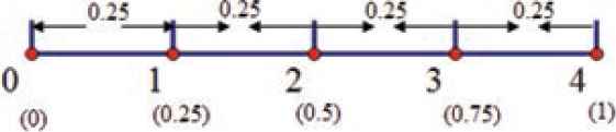
Suppose that the global optimal solution is 1 and the individual optimal solution is 3, then the adjusted spacing is
Adjusted spacing:
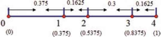
Next we follow the update strategy for each discrete variable: a random number uniformly distributed between 0 and 1 is generated by the computer. This number will fall into one of the intervals, the right value of this interval is defined as
For the example case shown above, if the random number is 0.625, then it will fall in the interval [0.5375, 0.8375], and so
Repeating the above process m times, the new discrete variable vector
2.4. Update Strategy for the Optimal Position Based on the Constraints
2.4.1. Update strategy of the personal best position
When the personal best position update is performed, we compare the current position
Let
For the two positions, there will be the following three situations in the comparison process (IDeb):
Both of the positions are feasible solutions (Gi = Gi,best = 0). In this case, it means that the two positions are in the feasible region, so the one having a better objective function value is preferred and made to be the current personal best position. Namely, when fi < fi,best, let
One position is a feasible solution, and the other one is an infeasible solution. In order to avoid losing the available information of the infeasible solution, we allow the infeasible solution to be accepted with a certain probability when the function value of the infeasible solution is less than the feasible solution in an early iteration. However, when the algorithm runs to the late stage, it is unacceptable that the infeasible solutions appear in the optimal position. So, the probability value of accepting infeasible solutions will be reduced to zero.
The probability function for accepting an infeasible solutions is
Both of the two positions are infeasible solutions (Gi > 0 and Gi,best > 0). At this point, it is not reasonable to only consider the constraint violation degree and ignore the information of the function value. Knowing how to reasonably balance the relationship between the function value and the constraint violation degree is very important. In this case, similarly to the multi-objective constraint handling method, all of the constraint functions are treated as an objective function.
When a dominant relationship exists, the solution will be compared by using a multi-objective constraint handling method. Namely, when the current position
If fi > fi,best and Gi < Gi,best or fi < fi,best and Gi > Gi,best, a dominant relationship does not exist. Thus, in order to better measure the relationship between the function value and the constraint violation degree, we define two new parameters. Consider case 1, as an example:
Constraint violation multiple:
Function value optimization multiple:
In case 1, the function value of Pi,best is smaller than the function value of
In case 2, the same conclusion can also be obtained.
By merging the above three cases, the pseudocode of the update strategy for the personal best position is as follows:
IDeb
1) Input:
Pi,best: the personal best position;
Pr: the probability value of accepting infeasible solutions;
2) If Gi = Gi,best = 0 (Both positions are feasible solutions.)
3) If fi < fi,best
4)
5) End If
6) Elseif Gi > 0, Gi,best = 0 (One position is a feasible solution, and the other one is an infeasible solution.)
7) If fi < fi,best
8) Randomly generate r ∈ [0, 1];
9) If r < Pr
10)
11) End If
12) End If
13) Elseif Gi = 0, Gi,best > 0
14) If fi < fi,best
15)
16) Else
17) Randomly generate r ∈ [0, 1];
18) If r > Pr
19)
20) End if
21) End if
22) Elseif Gi > 0, Gi,best > 0(Both positions are infeasible solutions.)
23) Calculate fmuli and Gmuli
24) If fi < fi,best & Gi < Gi,best
25)
26) Elseif fi > fi,best & Gi < Gi,best
27) If Gmuli > fmuli
28)
29) End If
30) Elseif fi < fi,best & Gi > Gi,best
31) If Gmuli < fmuli
32)
33) End If
34) End If
35) End If
The pseudocode of the update strategy for the personal best position.
2.4.2. Update strategy for the global best position
In the PSO algorithm, the guiding role of the global best position is considered as the social cognition of the population in the optimization process. Here, when the best optimal solution in the feasible solutions for the current population is better than the existing optimal solution, the global best position is updated. If there is no feasible solution in this generation, the global best position is not updated.
2.5. Description of the EMPSO
As previously analyzed, the details of EMPSO can be summarized as follows and the flowchart of EMPSO is given in Figure 1.
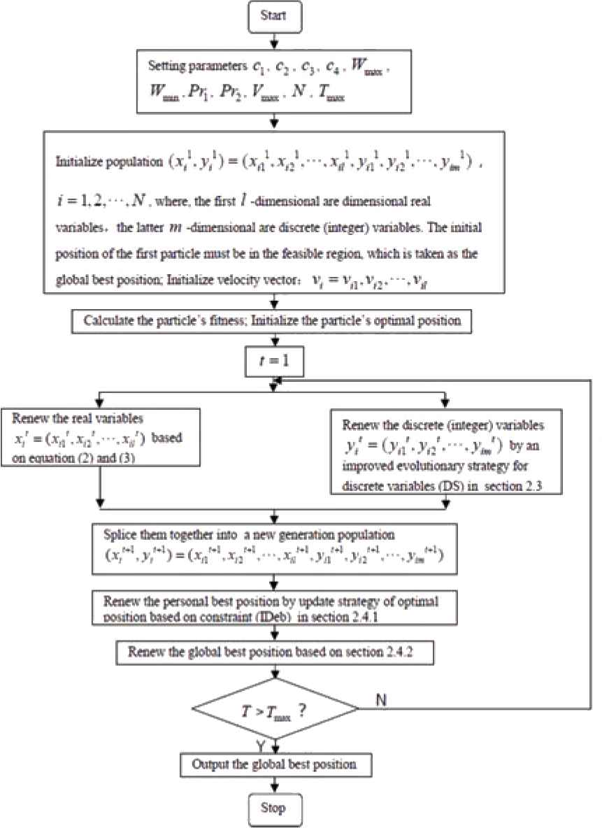
Flowchart of the efficient modified particle swarm optimization (EMPSO) algorithm.
Step 1: Initialize the position and velocity of each particle randomly in the search space:
Set the parameters c1, c2, c3, c4, wmax, wmin, Pr1, Pr2, the maximum generation Tmax, and the population size N. Also set t = 0.
Randomly initialize the positions of the population of particles by integer and continuous hybrid coding techniques and the velocities of the population of particles by continuous coding techniques.
Step 2: Calculate the objective function values from the initial positions of the particles, set the personal best position Pi,best of each particle equal to its current position, and set the global best position gbest.
Step 3: Update the continuous variables using Equations (2) and (3), and update the discrete variables by using the new evolutionary strategies described in Section 2.3.
Step 4: Update the personal best position Pi,best for i = (1, 2, ⋯ , m), and the global best position gbest, by using the update strategies described in Section 2.4.
Step 5: If the termination criterion is satisfied, then output gbest and its fitness value. If not, set t : = t + 1 and go to Step 2.
3. NUMERICAL SIMULATIONS
3.1. Test Problems and Experimental Setup
To demonstrate the effectiveness and performance of the EMPSO, 14 test problems selected from published literature, were solved. The salient features of the test problems are shown in Table 1. For the sake of completeness, a summary of these benchmark problems is given in the Appendix A.
| Problem | Total Number of Variables | Number of Integer Variables | Number of Constraints Excluding Bounds on Variables | References | |
|---|---|---|---|---|---|
| Inequality | Equality | ||||
| 1 | 2 | 1 | 2 | – | [2, 13] |
| 2 | 2 | 1 | 1 | – | [2, 13] |
| 3 | 3 | 1 | 3 | – | [2, 13] |
| 4 | 5 | 3 | 3 | 2 | [2] |
| 5 | 7 | 4 | 9 | – | [2] |
| 6 | 5 | 2 | 3 | – | [2] |
| 7 | 2 | 1 | 2 | – | [13] |
| 8 | 3 | 2 | – | – | [13] |
| 9 | 3 | 1 | 2 | – | [2] |
| 10 | 2 | 2 | 2 | – | [2] |
| 11 | 3 | 3 | 2 | – | [13] |
| 12 | 5 | 5 | 6 | – | [13] |
| 13 | 7 | 7 | 7 | – | [13] |
| 14 | 4 | 4 | 3 | – | [13] |
Salient features of the test problems.
In order to better study the effectiveness of the two improvement strategies (DS and IDeb) of the EMPSO algorithm, the classical evolutionary strategies for discrete variables, INT (update the discrete variables by a continuous evolution strategy, and then round), and Deb (an update strategy based on feasible solution priority, as previously described), were also studied. The experiments compare the EMPSO algorithm with other hybrid PSO algorithms: The INT-Deb-PSO algorithm and the DS-Deb-PSO algorithm. In the strategies mentioned above, common parameters to the three algorithms were set as follows: the self-cognitive coefficient for the continuous variables c1 = 1.7, the social cognitive coefficient for the continuous variables c2 = 1.7, the maximum inertia weight wmax = 0.9, the minimum inertia weight wmin = 0.5, and the maximum generation Tmax = 1000. In the EMPSO algorithm, the social cognitive coefficient for the discrete variables was set to c3 = 1.5, the self-cognitive coefficient for the discrete variables to c4 = 1.2, the minimum probability of accepting an infeasible solutions Pr1 = 0, and the maximum probability of accepting an infeasible solutions to Pr2 = 0.5. All programs were coded in Matlab and all executions were made on a Tsinghua Tongfang personal computer with an Intel(R) Core(TM) i5-3570K CPU@3.40 GHz.
3.2. Experimental Results
The 14 test problems were executed in 50 independent runs. Experimental results obtained by the three algorithms are given in Table 2, where “Fun.” indicates the problem, “Best” stands for the best optimal value obtained by the algorithm in all runs, “Worst” is the worst optimal value found by the algorithm in all runs, “Median” is the middle value of all obtained optimal values through the algorithm, “Mean” denotes the mean value of all obtained optimal values for the algorithm, “Std” is the standard deviation of all obtained optimal values through the algorithm, and “Success rate” represents the percentage of successful runs to the total runs for the algorithm (a successful run is where the obtained objective function value is within 0.1% of the known optimal value). Furthermore, “time” represents the average computation time (in seconds) used by the algorithm (in the case of successful runs), and “Avg. fun. eval.” is average number of objective function evaluations used by the algorithm in successful runs. The success rates of the three algorithms are shown in Figure 2.
| Fun. | Algorithm | Best | Worst | Median | Mean | Std | Success Rate | Time | Avg. Fun. Eval. |
|---|---|---|---|---|---|---|---|---|---|
| EMPSO | 2.000003 | 2.000100 | 2.000047 | 2.000051 | 9.54E-10 | 1 | 0.09 | 3307 | |
| 1 | DS-Deb-PSO | 2.000005 | 2.000100 | 2.000045 | 2.000050 | 6.36E-10 | 1 | 0.14 | 5315 |
| INT-Deb-PSO | 2.000001 | 2.236068 | 2.000048 | 2.009489 | 2.18E-03 | 0.96 | 0.04 | 5189 | |
| EMPSO | 2.124468 | 2.124499 | 2.124486 | 2.124484 | 1.01E-10 | 1 | 0.07 | 2311 | |
| 2 | DS-Deb-PSO | 2.124346 | 2.124499 | 2.124484 | 2.124479 | 5.46E-10 | 1 | 0.09 | 3448 |
| INT-Deb-PSO | 2.124349 | 2.124499 | 2.124477 | 2.124452 | 2.94E-09 | 1 | 0.03 | 2665 | |
| EMPSO | 1.076544 | 1.076839 | 1.076550 | 1.076556 | 1.67E-09 | 1 | 0.17 | 6406 | |
| 3 | DS-Deb-PSO | 1.076544 | 1.250000 | 1.076551 | 1.102258 | 3.63E-03 | 0.84 | 0.24 | 9151 |
| INT-Deb-PSO | 1.076545 | 1.350507 | 1.076551 | 1.118517 | 5.89E-03 | 0.74 | 0.07 | 6798 | |
| EMPSO | 7.667180 | 7.667180 | 7.667180 | 7.667180 | 7.24E-30 | 1 | 0.00 | 114 | |
| 4 | DS-Deb-PSO | 7.666911 | 8.740312 | 7.667180 | 7.737174 | 5.46E-10 | 0.92 | 0.17 | 3135 |
| INT-Deb-PSO | 7.667180 | 8.740215 | 7.667180 | 7.803010 | 1.05E-01 | 0.84 | 0.00 | 200 | |
| EMPSO | 4.579613 | 5.632730 | 4.579679 | 4.600734 | 2.22E-02 | 0.98 | 11.54 | 150992 | |
| 5 | DS-Deb-PSO | 4.579632 | 5.632730 | 4.579685 | 4.642862 | 6.38E-02 | 0.94 | 8.50 | 111262 |
| INT-Deb-PSO | 4.579641 | 5.780000 | 4.579695 | 4.940220 | 2.84E-01 | 0.68 | 1.40 | 124306 | |
| EMPSO | −32217.427471 | −32217.426018 | −32217.426489 | −32217.426579 | 1.47E-07 | 1 | 2.73 | 66672 | |
| 6 | DS-Deb-PSO | −32217.427739 | −32215.812744 | −32217.420663 | −32217.320323 | 9.54E-02 | 0.8 | 6.66 | 159860 |
| INT-Deb-PSO | −32217.427353 | −28674.167359 | −32217.426388 | −32146.470479 | 2.51E + 05 | 0.94 | 0.08 | 8219 | |
| EMPSO | −4242.004672 | −4242.003706 | −4242.004106 | −4242.004124 | 8.14E-08 | 1 | 0.62 | 22022 | |
| 7 | DS-Deb-PSO | −4242.004372 | −4241.997047 | −4242.003737 | −4242.002696 | 3.91E-06 | 0.62 | 0.78 | 28168 |
| INT-Deb-PSO | −7189.179772 | −1142.244867 | −4242.004209 | −3737.029756 | 2.42E + 06 | 0.72 | 0.07 | 7256 | |
| EMPSO | 0.000000 | 0.000001 | 0.000001 | 0.000001 | 7.05E-14 | 1 | 1.32 | 26314 | |
| 8 | DS-Deb-PSO | 0.000000 | 0.000001 | 0.000000 | 0.000000 | 8.66E-14 | 1 | 1.40 | 27814 |
| INT-Deb-PSO | 0.000000 | 0.000001 | 0.000001 | 0.000001 | 8.22E-14 | 1 | 0.17 | 8350 | |
| EMPSO | −75.134137 | −75.134000 | −75.134023 | −75.134039 | 1.36E-09 | 1 | 0.60 | 26654 | |
| 9 | DS-Deb-PSO | −75.134150 | −75.134000 | −75.134033 | −75.134043 | 1.40E-09 | 1 | 0.63 | 27948 |
| INT-Deb-PSO | −75.134118 | 15.532925 | 5.385932 | −28.057187 | 1.91E + 03 | 0.44 | 0.23 | 24141 | |
| EMPSO | −42.632121 | −42.632121 | −42.632121 | −42.632121 | 5.15E-29 | 1 | 0.00 | 60 | |
| 10 | DS-Deb-PSO | −42.632121 | −42.632121 | −42.632121 | −42.632121 | 5.15E-29 | 1 | 0.00 | 67 |
| INT-Deb-PSO | −42.632121 | −42.632121 | −42.632121 | −42.632121 | 5.15E-29 | 1 | 0.00 | 85 | |
| EMPSO | −68.000000 | −68.000000 | −68.000000 | −68.000000 | 0 | 1 | 0.02 | 436 | |
| 11 | DS-Deb-PSO | −68.000000 | −68.000000 | −68.000000 | −68.000000 | 0 | 1 | 0.03 | 593 |
| INT-Deb-PSO | −90.000000 | 16.000000 | −68.000000 | −65.840000 | 1.59E + 02 | 0.84 | 0.01 | 744 | |
| EMPSO | 8.000000 | 8.000000 | 8.000000 | 8.000000 | 0 | 1 | 0.01 | 119 | |
| 12 | DS-Deb-PSO | 8.000000 | 8.000000 | 8.000000 | 8.000000 | 0 | 1 | 0.04 | 440 |
| INT-Deb-PSO | 8.000000 | 14.000000 | 8.000000 | 8.120000 | 7.20E-01 | 0.98 | 0.00 | 86 | |
| EMPSO | 14.000000 | 14.000000 | 14.000000 | 14.000000 | 0 | 1 | 0.19 | 1680 | |
| 13 | DS-Deb-PSO | 14.000000 | 14.000000 | 14.000000 | 14.000000 | 0 | 1 | 0.22 | 2023 |
| INT-Deb-PSO | 14.000000 | 29.000000 | 14.000000 | 17.060000 | 2.12E + 01 | 0.56 | 0.04 | 4155 | |
| EMPSO | −0.974565 | −0.974565 | −0.974565 | −0.974565 | 4.53E-31 | 1 | 0.02 | 254 | |
| 14 | DS-Deb-PSO | −0.974565 | −0.974565 | −0.974565 | −0.974565 | 4.53E-31 | 1 | 0.03 | 391 |
| INT-Deb-PSO | −0.974565 | 0.000000 | −0.974565 | −0.948732 | 2.08E-02 | 0.96 | 0.01 | 672 |
EMPSO, efficient modified particle swarm optimization.
Results obtained by the three algorithms on 14 benchmark problems.
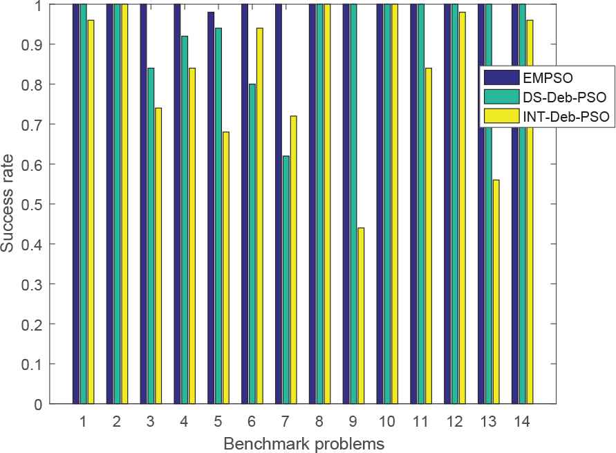
The success rates of three algorithms for 14 benchmark problems.
In order to reflect the optimization process, the optimizing curves of the three algorithms are plotted, in Figures 3–16, for the 14 test problems. For each image combination, the left image is the entire optimization process for the problem. As the main optimization process of some functions only takes place in a short period of time, the convergence process is not obvious in the left image. Therefore, in the right image, the part that converges fast for each function is locally enlarged.
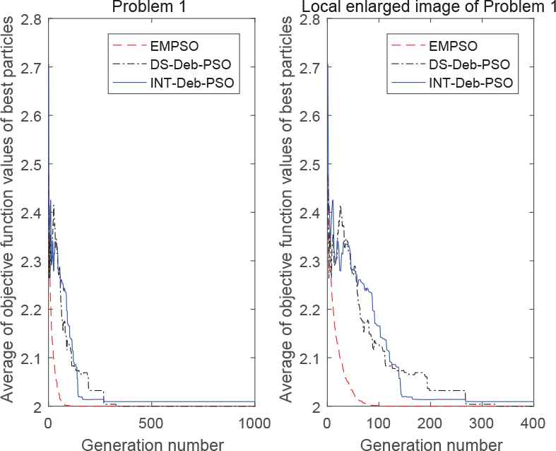
The entire (left) and locally enlarged (right) optimization curves for test problem 1.
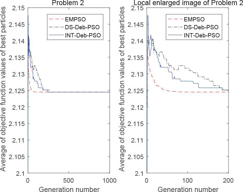
The entire (left) and locally enlarged (right) optimization curves for test problem 2.
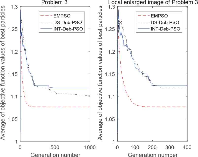
The entire (left) and locally enlarged (right) optimization curves for test problem 3.
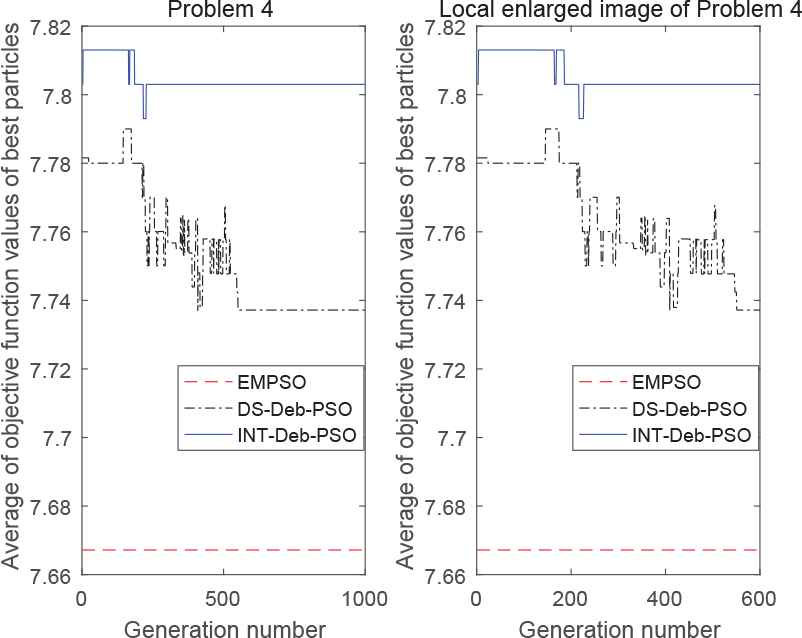
The entire (left) and locally enlarged (right) optimization curves for test problem 4.
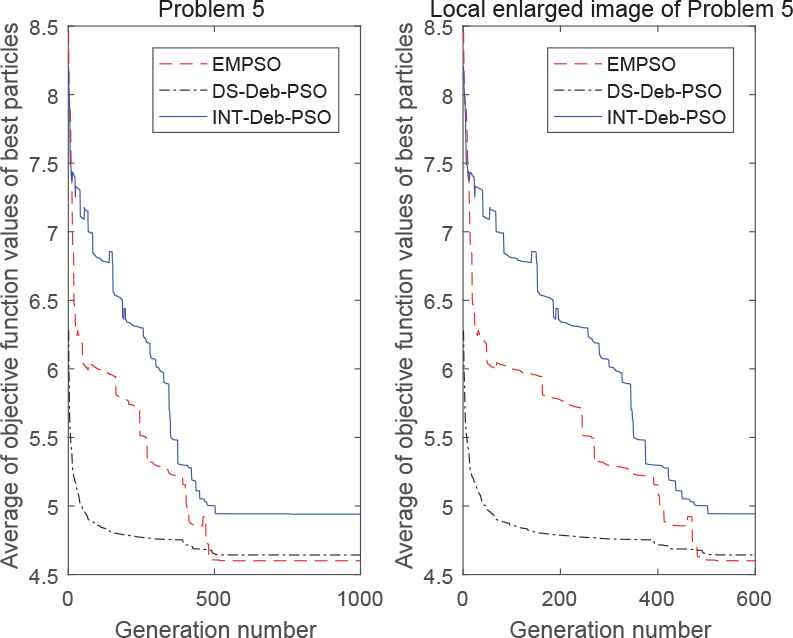
The entire (left) and locally enlarged (right) optimization curves for test problem 5.
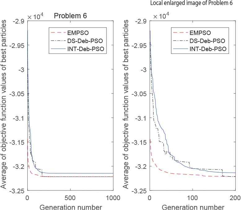
The entire (left) and locally enlarged (right) optimization curves for test problem 6.
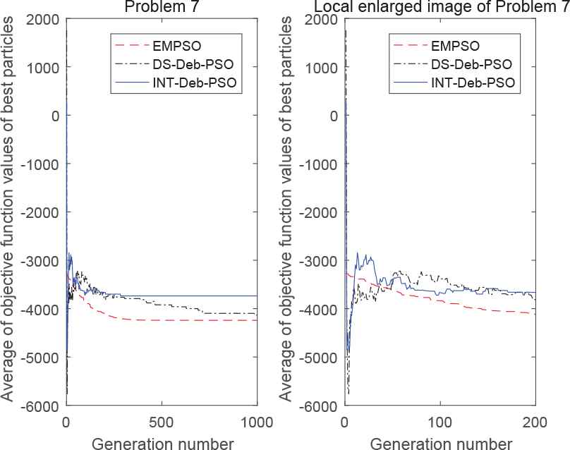
The entire (left) and locally enlarged (right) optimization curves for test problem 7.
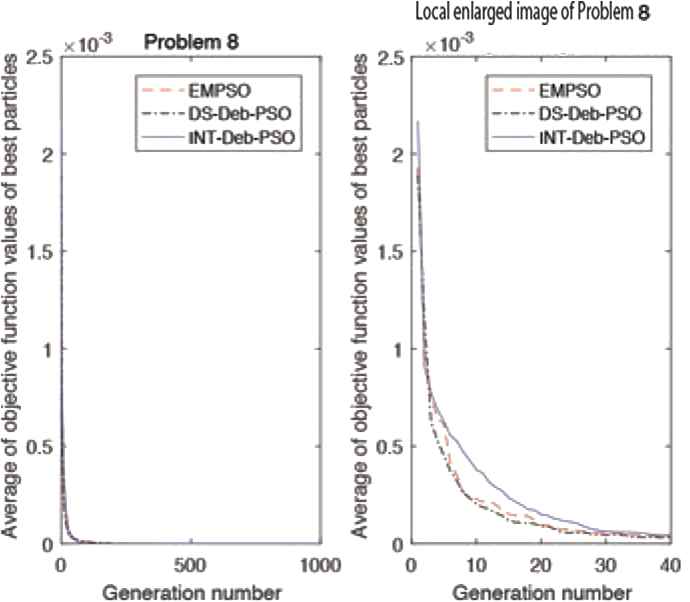
The entire (left) and locally enlarged (right) optimization curves for test problem 8.
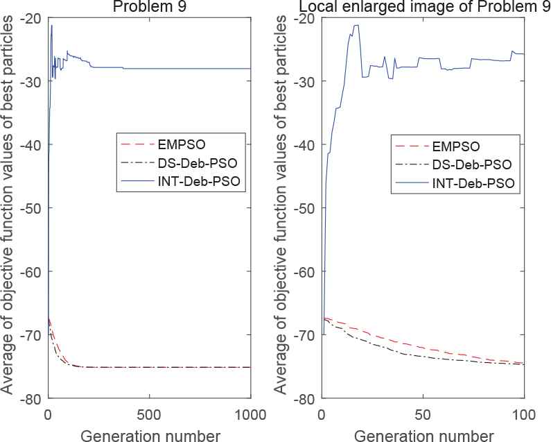
The entire (left) and locally enlarged (right) optimization curves for test problem 9.
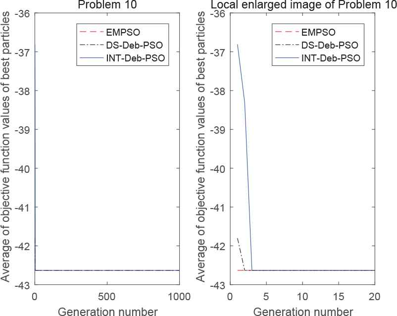
The entire (left) and locally enlarged (right) optimization curves for test problem 10.
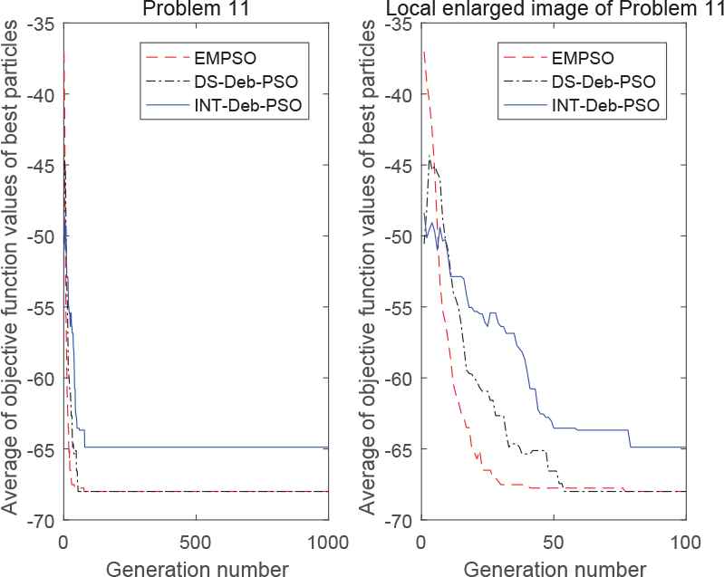
The entire (left) and locally enlarged (right) optimization curves for test problem 11.
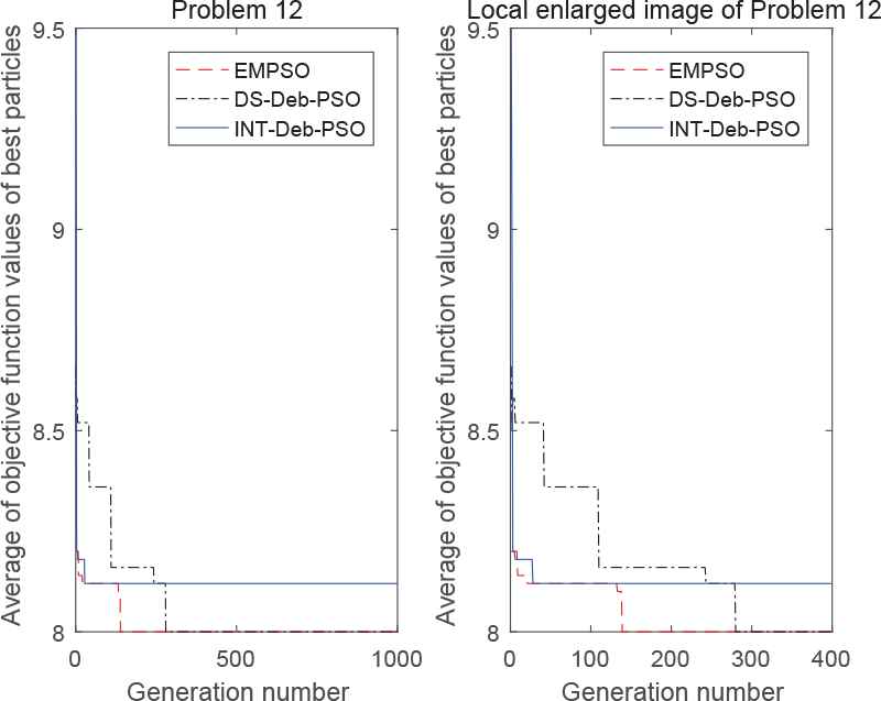
The entire (left) and locally enlarged (right) optimization curves for test problem 12.
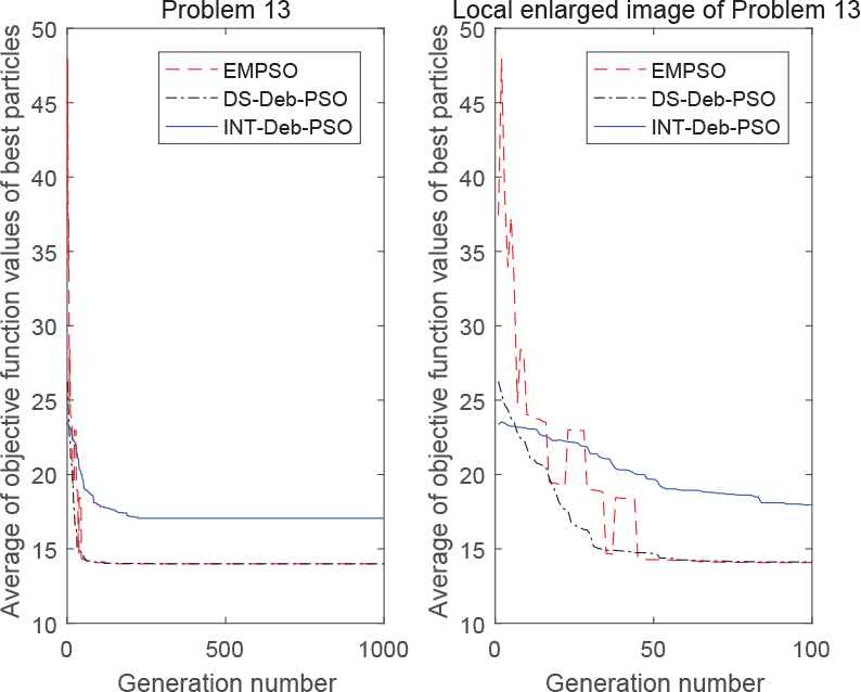
The entire (left) and locally enlarged (right) optimization curves for test problem 13.
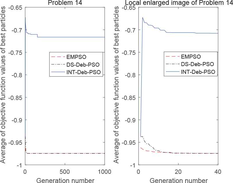
The entire (left) and locally enlarged (right) optimization curves for test problem 14.
3.3. Discussion of the Results
The results in Table 1 and Figure 2 show that EMPSO had the highest success rate in solving the 14 problems and provided a 100% success rate in 13 problems (i.e., all except for problem 5). Likewise, DS-Deb-PSO and INT-Deb-PSO provided a 100% success rate in 9 problems (1, 2, and 8–14) and 3 problems (2, 8, and 10), respectively. INT-Deb-PSO only had good performance in solving the problem with two continuous discrete variables, but for problem P9, which had nonuniformly spaced integers, its success rate dropped to 44%. Therefore, a combination of the DS strategy and the IDeb strategy is much better than the combination of the INT strategy and the Deb strategy. Since the DS strategy is more complex than the INT strategy, the computation time of the INT-Deb-PSO is the shortest, except for problem P4.
In terms of the average number of objective function evaluations, INT-Deb-PSO had the best value for five cases (6–9 and 12), whereas DS-Deb-PSO had the best value in only one case (5). In the other eight cases EMPSO obtained the best values. It can be seen that INT-Deb-PSO has obvious advantages in terms of computation time because of its simple strategy, but the advantage of the best average number of objective function evaluations is not as good as the algorithm based on the DS strategy.
EMPSO obtained the minimum standard deviation in all problems, and DS-Deb-PSO had a better standard deviation than INT-Deb-PSO for 13 problems (all except problem 8). The INT-Deb-PSO algorithm is not stable and fluctuates violently because of its lower success rate, and its standard deviation reached more than 10 for five problems (6, 7, 9, 11, and 13), it was as high as 106 for problem 7.
The known optimal solution could be obtained by EMPSO and DS-Deb-PSO, in our experiment, for all problems. For problems 7 and 11, INT-Deb-PSO seemed to have smaller experimental solutions than the known optimal solutions, but it could be easily verified that the two solutions were infeasible solutions. The EMPSO found the global optimal solutions within an acceptable error range (0.1%) for 13 problems and had an error of 0.02 for problem 5. The other algorithms were not 100% successful in solving all of the problems, as their error surpassed the allowed range. The algorithm with the DS strategy and the IDeb strategy, was not 100% successful in solving problems (such as problem 5), but its experimental solution was still near the known optimal solution and remained feasible. However, when other strategies are adopted, the deviation will increase, potentially generating infeasible experimental solutions.
In Figures 3–16, it appears that the EMPSO algorithm had a better convergence effect than the other algorithms, with its function curve dropping faster and smoother for all problems, except for problem 13. INT-Deb-PSO was not ideal in terms of the functional convergent curve of the 14 problems, having a slow convergence speed and poor stability. Furthermore, it could not converge to the optimal values for problems 6, 11, and 14. The convergence of DS-Deb-PSO was in between the other two algorithms. For problems 7, 11, and 13, the convergence speed of DS-Deb-PSO was faster than EMPSO at first, but it lagged behind the EMPSO algorithm before converging to the optimal value. The Deb strategy retained a feasible solution, so that the algorithm converged faster at an early stage. However, the Deb strategy ignored the guiding role of infeasible solutions, and so its ability to jump out of local optima was inferior to the IDeb strategy and the convergence effect was worse than the IDeb strategy at later stages.
Results from the above analysis show that each of the three algorithms had their own advantages in terms of time, success rate, average function evaluations, and average of the optimal solution. For INT-Deb-PSO, the computation time was obviously less than other algorithms, but the success rate was much lower than the other two algorithms. For test problem 5, the success rate of EMPSO was better than DS-Deb-PSO, but the computation time and average function evaluations of the EMPSO were inferior to DS-Deb-PSO.
3.4. Comparisons between the Three Algorithms with a New Performance Index
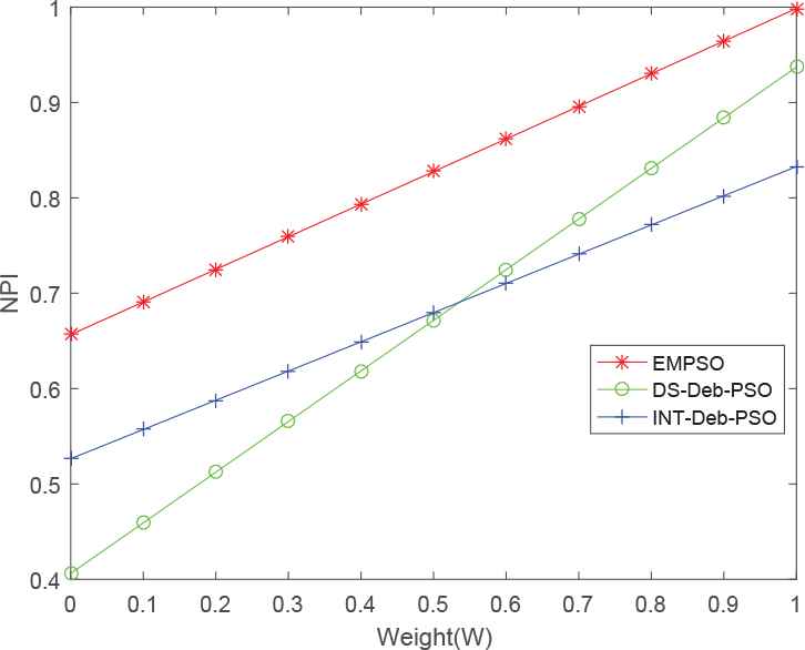
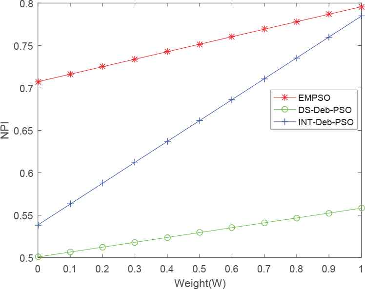
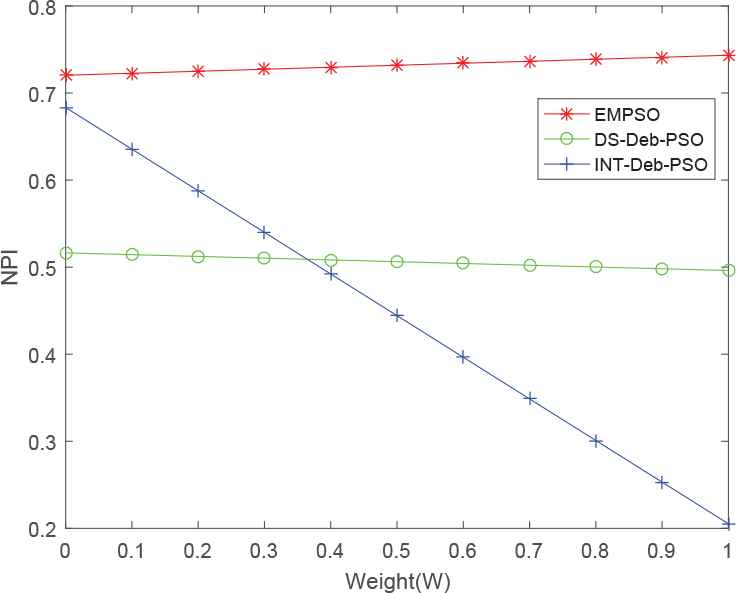
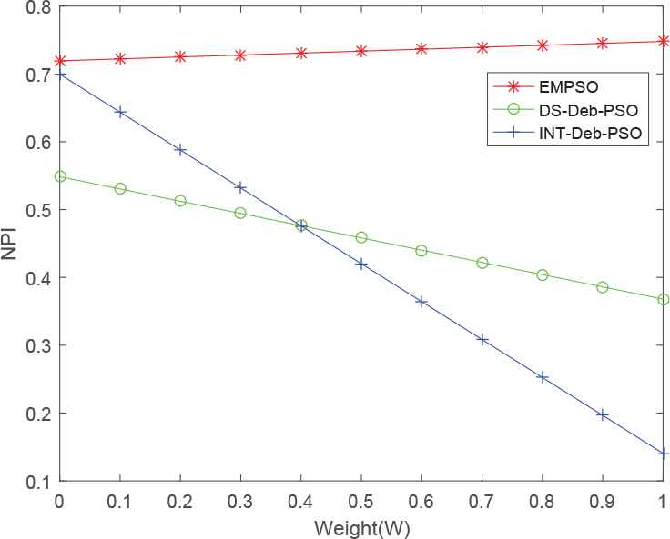
In order to get a better insight into the relative performance of computation time, success rate, and average function evaluations, the value of a performance index (PI) [18] is used. However, the PI cannot predict settlement in the stability of an algorithm and the distance between the calculated optimal value and the known optimal value, which are important in measuring the quality of an algorithm. In this paper, a new performance index (NPI) is proposed, based on an old PI, which is a comprehensive index of computation time, success rate, average function evaluations, stability of the algorithm, and the distance between the calculated optimal value and the known optimal value. For the computational algorithms we compared, the value of the new performance index NPIi for the algorithms is computed as
where N is the total number of test problems,
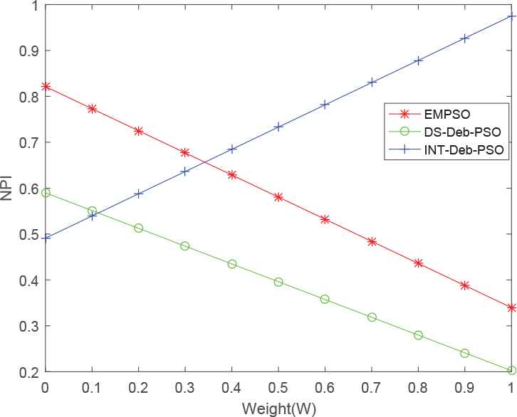
The graphs of NPI, corresponding to each of the five cases, are shown in Figures 17–21, respectively. It can be seen that the EMPSO algorithm outperformed the other two algorithms, except in Figure 18, in which the time was the main emphasis on the weights. In this case the evolutionary strategies for the discrete variables of the EMPSO algorithm, DS, need more time to calculate and are more complex than the approximate values (rounded-data) of INT-Deb-PSO. So, when k2 > 0.4, the NPI of EMPSO was surpassed by INT-Deb-PSO. The DS-Deb-PSO did not perform well under the comprehensive index NPI, the main reason being that the algorithm uses the DS strategy, which led to calculation times longer than INT-Deb-PSO, and the Deb strategy leads to the a lower convergence of efficiency than the EMPSO. In addition to the evolutionary strategies for the discrete variables and the update strategy, the other parameters of the three algorithms are the same, so we can see that the EMPSO, with the evolutionary strategies of the discrete variables (DS) and an update strategy based on the constraints (IDeb), was much more effective than the other hybrid-PSO algorithms; those with approximate values (INT) or an update strategy based on feasible solution priority (Deb).
New performance indices (NPIs) for the efficient modified particle swarm optimization (EMPSO), DS-Deb-PSO, and INT-Deb-PSO algorithms when
New performance indices (NPI) for the efficient modified particle swarm optimization (EMPSO), DS-Deb-PSO, and INT-Deb-PSO algorithms when
New performance indices (NPI) for the efficient modified particle swarm optimization (EMPSO), DS-Deb-PSO, and INT-Deb-PSO algorithms when
New performance indices (NPI) for the efficient modified particle swarm optimization (EMPSO), DS-Deb-PSO, and INT-Deb-PSO algorithms when
New performance indices (NPI) for the efficient modified particle swarm optimization (EMPSO), DS-Deb-PSO, and INT-Deb-PSO algorithms when
3.5. Comparison of the Computational Complexity of the Three Algorithms
In this section, in order to further compare the advantages and disadvantages of the three algorithms, the computational complexity of the proposed three algorithms is discussed. Since the main program of the three algorithms is the same, both the time and space complexities of the different improvement strategies in one generation are analyzed below.
3.5.1. Time complexity
INT Strategy:
Updating the discrete variables by the continuous update strategy of the PSO (the position and velocity are updated) requires O (N * m time, where N indicates the population size and m indicates the dimension of the discrete variable.
The rounding operation requires O (N * m) time.
Hence, the total time complexity of the INT strategy is O (N * m).
DS Strategy:
Calculating the standard spacing requires O (m) time.
Calculating the adjusted spacing requires O (N * m) time.
Determining the update interval requires O (N * m) time.
Updating the position vector requires O (N * m) time.
Hence, the total time complexity of the DS strategy is O (N * m).
Deb Strategy:
Calculating the constraint violation degree requires O (N * m) time, where L indicates the number of constraint functions.
Calculating the fitness values of the current position and the personal best position requires O (N) time.
Updating the personal best position requires O (N) time.
Hence, the total time complexity of the Deb strategy is O (N * m).
IDeb Strategy:
In the worst case,
Calculating the constraint violation degree requires O (N * m) time.
Calculating the fitness values of the current position and the personal best position require O (N) time.
Calculating the constraint violation multiple requires O (N) time.
Calculating the function value optimization multiple requires O (N) time.
Updating the personal best position requires O (N) time.
Hence, the total time complexity of the IDeb strategy is O (N * m).
In summary, we can see that the time complexities of the INT and DS strategies are on the same order. However, it is not difficult to find that the former is easy to operate, and so its calculation frequency is smaller than the latter. Additionally, the time complexity of the Deb strategy is smaller than that of the IDeb strategy, but the gap is very small. Therefore, the computation time of INT-Deb-PSO is the smallest, compared with the other two algorithms, which can also be seen in Figure 18. This is the advantage of the INT-Deb-PSO algorithm, but its performance in other aspects is not good. It can be seen that the calculation effect of the EMPSO algorithm is better; while the computation time is longer than the others, they basically remain on the same order.
3.5.2. Space complexity
INT Strategy:
As the update of the discrete variables needs to be overwritten in the calculation process, and no additional storage is needed. Hence, the space complexity is O (N * m).
DS Strategy:
The amount of space taken up by storing the spacing vector is O (N * |Ωmax| * m), where |Ωmax| = max{|Ωd|, d = 1, 2, ⋯ , m}.
The update of the discrete variables needs to be overwritten in the calculation process, so the amount of space is O (N * m).
Hence, the total space complexity of the DS strategy is O (N * |Ωmax| * m).
Deb Strategy:
The amounts of space taken up by the constraint violation degree of the current position and the personal best position are O (N).
The amounts of space taken up by fitness values of the current position and the personal best position are O (N).
The amounts of space taken up by the current position and the personal best position are O (N * d), where d indicates the dimension of the particle.
Hence, the total space complexity of the Deb strategy is O (N * d).
IDeb Strategy:
In the worst case,
The amounts of space taken up by the constraint violation degree of the current position and the personal best position are O (N).
The amounts of space taken up by fitness values of the current position and the personal best position are O (N).
The amount of space taken up by the constraint violation multiple is O (N).
The amount of space taken up by the function value optimization multiple is O (N).
The amounts of space taken up by the current position and the personal best position are O (N * d).
Hence, the total space complexity of the IDeb strategy is O (N * d).
We can see that the two improved strategies (DS and IDeb) take up a little more space than the two classical strategies (INT and Deb). However, for the current level of computer hardware, the impact of these additional storage requirements on the operation of the algorithm is basically negligible.
To summarize, the EMPSO algorithm not only improves the computational accuracy, but also achieves acceptable computational time and space occupancy.
4. CONCLUSIONS
This paper has presented an EMPSO for solving mixed integer nonlinear programming problems. For comparison, two hybrid PSO algorithms, the INT-Deb-PSO algorithm and the DS-Deb-PSO algorithm, were also implemented. All three algorithms have two evolutionary strategies: the evolutionary strategies of the discrete variables (DS or INT) and an update strategy of the optimal position (IDeb or Deb). For 14 integer and MIP problems, the numeric results show that EMPSO has a better robustness and faster convergence speed than the other two hybrid PSO algorithms. In order to fairly compare EMPSO with the other hybrid PSO algorithms, a comprehensive index, NPI, is proposed in this paper, which can weigh the importance of computation time, success rate, average number of function evaluations, stability of the algorithm, and the distance between the calculated optimal value and the known optimal value. The value of the NPI obtained by EMPSO is superior to the other algorithms in most cases, but the computational time of EMPSO needs to be further reduced. In this article, we only deal with the MIP problems with one objective function. In the near future, we also plan to deal with the MIP problems with multi-objective. Furthermore, most parameters in this paper (such as c3, c4, etc.) have certain values. It would be interesting to study whether these control parameters could adaptively change as the iteration time increases.
ACKNOWLEDGMENTS
This research was funded by the National Natural Science Foundation of P.R. China (61561001), First-Class Disciplines Foundation of NingXia (Grant No. NXYLXK2017B09) and Major Project of North Minzu University (2019MS003).
APPENDIX A
0–1 mixed integer nonlinear programming problems
The known optimal solution: F* = 2, x = 0.5, y = 1.
The known optimal solution: F* = 2.1247, x = 1.375, y = 1.
The known optimal solution: F* = 1.076543, x = [0.94194, −2.1], y = 1.
The known optimal solution: F* = 7.667, x = [1.117, 1.310], y = {0,1,1}.
The known optimal solution: F* = 4.5796, x = [0.2, 0.8, 1.908], y = {1, 1, 0, 1}.
Mixed integer nonlinear programming (uniformly spaced integer)
The known optimal solution: F* = −32217.4, x = [27, any, 27], y = {78, any}.
The known optimal solution: F* = −4242.00473, x = 3.65464, y = 15
The known optimal solution: F* = 0, x = 1.5, y = {50, 25}
Mixed integer nonlinear programming (nonuniformly spaced integer)
The known optimal solution: F* = −75.1341, x = [13.4, 5.6070],y = 500
Integer nonlinear programming
The known optimal solution: F* = −42.632, y = {1,3}
The known optimal solution: F* = −68, y = {2, 0, 5}
The known optimal solution: F* = 8, y = {1, 1, 1, 1, 2}
The known optimal solution: F* = 14, y = {0, 2, 4, 0, 2, 1, 4}
The known optimal solution: F* = −0.974565, y = {3, 3, 2, 3}
REFERENCES
Cite this article
TY  - JOUR
AU  - Ying Sun
AU  - Yuelin Gao
PY  - 2019
DA  - 2019/04/12
TI  - An Efficient Modified Particle Swarm Optimization Algorithm for Solving Mixed-Integer Nonlinear Programming Problems
JO  - International Journal of Computational Intelligence Systems
SP  - 530
EP  - 543
VL  - 12
IS  - 2
SN  - 1875-6883
UR  - https://doi.org/10.2991/ijcis.d.190402.001
DO  - 10.2991/ijcis.d.190402.001
ID  - Sun2019
ER  -