
Improved TODIM Method Based on Linguistic Neutrosophic Numbers for Multicriteria Group Decision-Making
- DOI
- 10.2991/ijcis.d.190412.001How to use a DOI?
- Keywords
- TODIM; Linguistic neutrosophic numbers; Score function; Combined weight model; MCGDM
- Abstract
The TODIM (an acronym in Portuguese for interactive multicriteria decision-making) method can consider the decision-makers’ (DMs’) psychological behavior. However, the classical TODIM method has been unable to address fuzzy information such as the linguistic neutrosophic number (LNN), which is an effective tool to represent uncertainty. In this paper, an extended TODIM method is proposed to solve multicriteria group decision-making (MCGDM) problems in a linguistic neutrosophic environment. First, the definitions and characteristics of the classical TODIM and the LNNs are introduced. Then, an improved score function (SF) of LNNs is proposed. Furthermore, we obtain the combined weights of the criteria and aggregate individual decision matrices into a group decision matrix. The classical TODIM method is extended to address MCGDM problems with LNNs, and specific decision steps are provided. Finally, several examples are given to verify the effectiveness and superiority of the proposed approach by comparison with some existing methods.
- Copyright
- © 2019 The Authors. Published by Atlantis Press SARL.
- Open Access
- This is an open access article distributed under the CC BY-NC 4.0 license (http://creativecommons.org/licenses/by-nc/4.0/).
1. INTRODUCTION
As practical decision situations have become more complex, we should consider how to better express evaluation information and make optimal judgment by appropriate decision methods for multicriteria decision-making (MCDM) or multicriteria group decision-making (MCGDM) problems. There are numerous methods to describe the evaluated object [1–6], such as fuzzy set (FS), intuitionistic fuzzy set (IFS), neutrosophic set (NS), and so on. Due to the uncertainty in decision environments and the cognitive limitations of human beings, Zadeh first proposed [6] FSs to present fuzzy evaluation information by using truth membership (TM). Based on the FS, Atanassov presented [1] IFSs that consist of TM and the falsity membership (FM). However, IFSs can only address incomplete information but not uncertain and inconsistent information. Then, Smarandache introduced [2] NSs to describe indeterminate and inconsistent information where each element of the universe is represented by TM, FM, and indeterminacy membership (IM). In view of their advantages, NSs have been applied in an increasing number of fields to help decision-makers (DMs) make rational and feasible judgements. For instance, Ye defined [7] two cotangent similarity measures based on NSs and a cotangent function and applied them to the fault diagnosis of a steam turbine. Zavadskas et al. introduced [8] a MAMVA model for NSs in the construction industry. Bolturk and Kahraman developed [9] a new method for MCDM problems by combining the interval-valued NSs and analytic hierarchy process (AHP). Abdelbasset et al. advanced [10] the idea that associated an NS with a mining algorithm that can effectively extract information from big data. Rashno et al. utilized [11] NSs and graph algorithms to present a fully automated algorithm in the healthcare industry. Fan et al. proposed [12] a neutrosophic Hough transform (NHT) method to improve the track initiation monitoring capacity in an uncertain environment.
In practice, people are used to giving their opinions in qualitative terms, such as “excellent,” “fair,” and “worse.” At this point, Zadeh defined [13] linguistic variables (LVs) to describe words or sentences in natural language. Since then, many studies on linguistic decision-making problems have been conducted. Wu et al. put forward [14] the maximum support degree model to guarantee the accuracy of group opinion based on linguistic distributions. Zhang et al. established [15] a new decision support model with 2-tuple linguistic terms that provided a basis for emergency decision-making. Furthermore, there are many extensions of LVs to accurately express evaluation information. Based on the FS model, Rodríguez et al. proposed [16] the concept of a hesitant fuzzy linguistic term set (HFLTS) in which a DM may hesitate among several LVs to define the TM. Analogously, Chen and Liu defined [17] the linguistic intuitionistic fuzzy numbers (LIFNs) that represent the TM and FM by LVs. However, the above linguistic forms reflect only the TM (and FM), and thus they are insufficient to accommodate uncertain and inconsistent information. Therefore, Fang and Ye introduced [18] the concept of linguistic neutrosophic numbers (LNNs) based on NS, which is characterized by describing the TM, IM, and FM of each element in a universe using three LVs.
For MCGDM problems, there are two common methods to help DMs select the optimal proposal from a variety of alternatives. One method uses aggregation operators that integrate the evaluation information of the alternatives to form a comprehensive value. Because information loss occurs in the integration process of the aggregation operators, there is another method—the use of the traditional decision methods, such as AHP [19], TOPSIS [20], VIKOR [21], ELECTRE [22], and other approaches [23, 24]. All of the above methods assume that DMs are perfectly rational, which is not in accord with all practical situations. For such cases, Gomes and Lima proposed [25] the TODIM approach based on the prospect theory [26], which considers a DM’s psychological preference. Up to now, it has been widely used in the decision-making domain. Wei et al. extended [27] the TODIM method to HFLTSs based on a novel score function (SF) of HFLTSs. Ren et al. applied [28] the TODIM approach to a Pythagorean fuzzy environment for a MCDM problem. Lourenzutti et al. developed [29] a TODIM model based on the Choquet integral to address heterogeneous information with interactions. Hu et al. proposed [30] a new decision model by combining the TODIM method and a three-way decision model. Llamazares put forward [31] a generalization of the TODIM method that avoided the previous paradoxes.
In an actual decision-making process, due to the bounded rationality of the DMs, they may have different preferences when facing with a gain or a loss. Therefore, the TODIM approach is a good tool that can select appropriate and satisfying optimums for DMs. Moreover, LNNs can represent incomplete, inconsistent, and indeterminate information. Based on these analyses, it is a good idea to apply TODIM in a linguistic neutrosophic environment. It is understood that the significant characteristic of the TODIM approach is that it can reflect a DM’s risk preference in the face of a loss. Hence, the premise is that we need to judge a gain and a loss by a comparison of the LNNs. SF flaws exist in Reference [18] under some cases, such as the LNNs m1 = (s6, s2, s3) and m2 = (s5, s1, s3) ∈ Γ[0,6]; therefore, we cannot distinguish them from the existing SF of the LNNs. To address this, we will propose a revised SF to overcome this shortcoming. The revised SF can more effectively compare LNNs without the assistance of an accuracy function.
However, the criteria weights have an impact on the TODIM approach. There are three methods to obtain criteria weights: (i) subjective weight provided by the DMs; (ii) objective weight from the evaluation information; and (iii) combined weights that combine the DMs’ preference and the evaluation information. The subjective weights from the DMs reflect the judgment and knowledge of the DMs in a complex decision environment. The objective weights are based on the evaluation information and utilize mathematical models to obtain a solution. To obtain the reasonable criteria weights, we should consider both the DMs’ preferences and the evaluation information. Therefore, we will develop a combined weight model based on the subjective weights from the DMs and the objective weights obtained by projection measurement.
Based on the above analysis, this paper considers the bounded rationality of the DMs and the complicacy of the decision environment. An improved TODIM approach based on the revised SF of the LNNs and the combined weights of the criteria is proposed. In summary, the main innovations and contributions of this paper can be summarized as follows:
Define a revised SF of the LNNs and prove its relevant properties;
Develop a combined weight model based on the minimum deviation in which the subjective weights are given by the DMs and the objective weighs are obtained by projection measurement;
Provide a new approach for the MCGDM under a linguistic neutrosophic environment. Then, demonstrate the procedure of the proposed method in detail; and
Prove the validity and superiority of the proposed method by comparison with other existing methods.
To accomplish these goals, we constructed the framework of this paper as follows: Section 2 presents the basic theories and concepts including the linguistic term set (LTS), the single-valued NS (SVNS), the LNNs, and the TODIM method. Section 3 develops a revised SF and proves the associated properties. Section 4 establishes the combined weight model. Section 5 demonstrates the steps of the proposed method. Section 6 illustrates some examples and compares the proposed method with those existing approaches that have been presented in References [18, 32, 33]. Section 7 concludes this paper.
2. PRELIMINARIES
2.1. LTS and Linguistic Scale Function
An LTS St = {si | i = 0, 1, 2, …, 2t} is an ordered discrete term set that accommodates a list of LVs, where t ∈ N, N is a collection of natural numbers. Meanwhile, there are restrictions on St [13]:
The LTS St is ordered: si ≻ sj if and only if i > j;
A negation operator is defined as: neg (si) = s2t − i.
During the integration process, we usually convert LTs into numerical values by a linguistic scale function (LSF) that can reduce the loss of information.
Definition 1.
[34] Let St = {si | i = 1, 2, …, 2t} be a discrete LTS, si, be an LT. There exists a numerical value θi ∈ [0, 1], then the LSF is a mapping from si to θi (i = 0, 1, …, 2t), and it can be defined as follows:
Now, we introduce two types of LSFs [34]:
This function simply uses the subscript function to evenly distribute the semantic values of the linguistic information.
2.2. Single-Valued NSs
Definition 2.
[2] Let X be a fixed set with the elements in X marked as x, an NS, B, in X is characterized by TM, TB (x), IM, IB (x), and FM, FB (x). It can be defined as:
Meanwhile, there are TB (x), IB (x), FB (x) ∈ [0, 1] and 0 ≤ TB (x) + IB (x) + FB (x) ≤ 3 for each x in X.
To simplify the NS and exploit its wide application in various fields, Wang et al. advanced [4] the idea of the SVNS, which is an extension of the NS.
Definition 3.
[4] Let X be a fixed set with the elements in X marked as x, a SVNS, B, in X is defined as B = {〈x, TB (x), IB (x), FB (x) 〉| x ∈ X}, where TB (x), IB (x), and FB (x) denote the TM, IM, and FM of the element x ∈ X to the set B, respectively, and they are bounded by [0, 1], and 0 ≤ TB (x) + IB (x) + FB (x) ≤ 3.
For simplicity, we use x = (T, I, F) to represent an element, x, in the SVNS, which is called a single-valued neutrosophic number (SVNN).
2.3. Linguistic Neutrosophic Numbers
Definition 4.
[18] Let X be a fixed set and S = (s0, s1, …, s2t) be an LTS. The LNS M in X is composed of a TM, σM, an IM, θM, and an FM, τM, where σM, θM, τM: X → [0, 2t], and ∀x ∈ X,
To keep things simple, we use Γ[0, 2t] to represent the set of all of the LNNs.
Definition 5.
[18] Let m = (sσ, sθ, sτ),
Definition 6.
[32] Let X be the universe of discourse, where X = {x1, x2, …, xn}, and let M and N be two LNSs in X, where
Definition 7.
[18] Let
Definition 8.
[18] Let
2.4. The Traditional TODIM Method
The TODIM approach is proposed based on the prospect theory, which assumes that the rationality of the DMs is limited in the decision process. There is a different deviation between the optimal choice and DMs’ actual choice due to the DMs’ cognitive level, risk preference, and so on. Similar to prospect theory, the TODIM model defines a value function to reflect a gain or a loss for each criterion.
In the following, we will describe the specific steps of the TODIM method [25]:
Let
First, normalize the decision matrix
Second, define the relative weight of the criterion, Cj, to be the reference criterion, Cr as:
Next, calculate the dominance degree of alternative Ai over the alternative At by the following formula:
The θ can reflect the DM’s attitude about losses (θ > 0). In Equation (13), there will be three cases: (i) when zij − ztj ≻ 0, the ϕj (Ai, At) means a gain; (ii) when zij − ztj = 0, the ϕj (Ai, At) means a balance point; and (iii) when zij − ztj ≺ 0, the ϕj (Ai, At) means a loss.
Then, we can obtain the overall dominance degree of the alternative Ai by
Finally, rank the alternatives by their overall dominance degrees δ (Ai) (i = 1, 2, …, l). The greater δ (Ai) is, the better alternative Ai will be.
3. A NEW SF FOR LNNs
Although LNNs can depict the uncertain and imperfect evaluation information by LVs, we cannot directly compare two LNNs. Therefore, it’s necessary to develop a method to transform LNNs into crisp numbers. An SF is a good means to implement this requirement. Chen and Tan first proposed [35] a SF to address a fuzzy MCDM problem that evaluates the difference between the TM and FM. Obviously, it can effectively transform a fuzzy number into a crisp number and reflect the degree of suitability for each alternative. Similarly, Fang and Ye [18] provided the SF of a LNN and the definition is as follows:
Definition 9.
[18] Let m = (sσ, sθ, sτ) ∈ Γ[0, 2t], then the SF of a LNN m can be defined:
Example 1.
Let m1 = (s6, s2, s3), m2 = (s5, s1, s3) ∈ Γ[0, 6] be two LNNs, then
Thus, Fang and Ye [18] defined the accuracy function, α (m), where
In addition, there exists an obstacle for the LNN: how to evaluate and address the IM sθ. In this paper, we divide the IM into two parts in the SF, bθ, and (1 − b) θ, because there might be a FM and other parts may tend to be a TM or there might be other unknown and uncertain cases. For an LNN, we know that a higher value of the TM and a lower of the FM is better. Hence, the FM contained in the IM part of a SF should be subtracted rather than using the entire IM. In general, the percentage of the FM in an IM should be in accord with the percentage of the FM in the total evaluation value of the LNN in the same decision-making environment. Accordingly, b can be denoted as b = τ /σ + τ. For example, an LNN m = (s4, s3, s1) ∈Γ[0, 6], then b = 0.2. Therefore, based on the SF in Definition 9, a new SF is defined as
Notice that the new SF ψ′ (m) will not work in some extreme cases, such as
Theorem 1.
For an LNN m = (sσ, sθ, sτ) ∈ Γ[0, 2t], the new SF ψ′ (m) monotonically increases along with σ and monotonically decreases along with θ, τ.
Proof.
It is obvious that as σ increases, ψ′ (m) will monotonically increase. Similarly, ψ′ (m) will decrease with respect to θ.
For τ,
To prove the effectiveness of the new SF, we apply it in Example 1. There are
4. THE COMBINED WEIGHT MODEL BASED ON LNNs
The criteria weight is one of the important parameters considered in MCDM problems and plays a key role in the ranking alternatives. There are two common methods: subjective weighting approaches that focus primarily on the preferences of the DMs and objective weighting approaches that can be computed by the entropy [36], the distance [37], and the correlation coefficient [38]. Compared to the subjective weight models, the objective weight models can effectively reduce the subjectivity and improve the reliability, while they neglect the preferences of the DMs. To obtain scientific and proper weight information, they should not only consider the DMs’ preferences but also make full use of the objective evaluation information of the alternatives to achieve the unification of subjectivity and objectivity. Therefore, the combined weight model has a vital practical significance by reasonably combining the subjective weights and the objective weights. In this paper, we build a novel model to determine the criteria weights by combining the subjective factors with the objective factors that can be computed by projection measures. The characteristics of our weight model can reflect both the subjective judgment from a DM and the objective evaluation information. Next, we introduce how to obtain the objective weights. Then, by combining them with the given subjective weights, we will provide a combined weight model based on the minimum total deviation between the evaluation values with the combined weights and the original weights.
4.1. The Objective Weighted Model Based on Projection Measure
In a MCDM problem, suppose the alternative set is A = (A1, A2, ⋯, Al), and the criteria set is C = (C1, C2, ⋯, Ch) where the objective weight of criterion,
The projection measure is proposed from the point of a vector, which considers the evaluation value as a vector.
First, define the ideal solution from all of the alternatives, Ai(i = 1, 2, …., l), for each criterion, Cj, according to the SF by Equation (16), that is,
Then, obtain the projection values of the evaluation values for all of the alternatives of the ideal solution under the criterion Cj (j = 1, 2, …., h).
There is an angle between the evaluated values and the ideal solution, so we give the cosine formula between zij and
In the following, we define the projection of the criterion value, zij, on the ideal solution,
Obviously, the greater
To obtain the solution, we can construct the following Lagrange function:
4.2. The Combined Weight Model
To achieve the unification of the subjectivity and the objectivity, considering the subjective preferences and the empirical judgment of the DMs and the objective evaluation information, several combined weight methods have been proposed [39–41]. In this paper, our proposed combined weight model is based on the minimum total deviation between the evaluation values with the combined weights and the original weights.
We suppose the subjective weight,
To obtain the solution, we construct the following Lagrange function:
5. AN IMPROVED TODIM METHOD FOR MCGDM PROBLEMS WITH LNNs
In this section, we propose a novel method to solve MCDM problems with LNNs based on the improved TODIM method.
Let A = {A1, A2, …., Al} be a set of alternatives, C = {C1, C2, …., Ch} be the set of criteria, and D = {D1, D2, …., Dp} be the set of the DMs. The DM Dk gives the evaluation information of the alternative Ai under each criterion Cj by LNN, which is denoted
Step 1: Normalize the decision-making information.
If both the benefit criteria and the cost criteria are present in the decision matrix, we need to convert the different types of the criteria into the same type. The normalized decision matrix is denoted
Step 2: Obtain the comprehensive decision-making matrix.
We use the LNWAA operator or the LNWGA operator that was presented in Definition 7 or Definition 8, respectively, to obtain the comprehensive decision-making matrix
Step 3: Calculate the combined weights of the criteria.
First, define the ideal solution from all of the alternatives for each criterion, Cj, by Equation (16), that is,
Next, combine the given subjective weights provided by the DMs with the objective weights, and obtain the combined weights of the criteria based on Equations (22–24) found in Subsection 4.2.
Step 4: Obtain the relative weight,
Step 5: Calculate the dominance degree, ϑ (Ai, At), of alternative Ai over alternative At:
Step 6: Obtain the overall dominance degree of the alternative Ai by
Step 7: Rank the alternatives.
Sort the alternatives by their overall dominance degrees, δ (Ai). The bigger the overall dominance degree, δ (Ai), the better the alternative Ai.
6. APPLICATION EXAMPLE
In this section, we will first illustrate the procedure of the proposed MCGDM method by a specific example [32]. Then, we present some examples to demonstrate the effectiveness and superiority of the proposed MCGDM method by comparison with the existing MCGDM methods [18, 32, 33].
6.1 The Procedure of the Proposed Method
In this subsection, we will use an investment group decision-making example to demonstrate the application of the proposed method for MCGDM problems.
Example 5.1.
An investment company selects four mines, A1, A2, A3, and A4, as alternatives and considers five factors as the evaluation criteria: (i) C1 is the geology factor; (ii) C2 is the mineral reserve risk; (iii) C3 is the development level of the market; (iv) C4 is the construction project risk; and (v) C5 is the policy impact. The DMs, Dh(h = 1, 2, 3), gives the evaluation values of alternatives zAi (i = 1, 2, 3, 4) on the criteria Cj (j = 1, 2, 3, 4, 5) in the form of LNNs based on the LTSs: S = {s0 = extremely low, s1 = pretty low, s2 = low, s3 = slightly low, s4 = medium, s5 = slightly high, s6 = high, s7 = pretty high, s8 = perfect}. Assume that the weight vector of three DMs is
| C1 | C2 | C3 | C4 | C5 | |
|---|---|---|---|---|---|
| A1 | (s1, s2, s1) | (s2, s3, s2) | (s4, s4, s3) | (s1, s5, s1) | (s3, s3, s2) |
| A2 | (s2, s6, s2) | (s3, s8, s2) | (s2, s4, s1) | (s3, s1, s2) | (s1, s2, s1) |
| A3 | (s2, s3, s1) | (s3, s2, s3) | (s1, s4, s1) | (s3, s5, s1) | (s5, s2, s4) |
| A4 | (s3, s1, s2) | (s1, s7, s1) | (s4, s6, s3) | (s2, s5, s1) | (s4, s6, s4) |
LNN decision matrix Y1 given by D1.
| C1 | C2 | C3 | C4 | C5 | |
|---|---|---|---|---|---|
| A1 | (s1, s6, s1) | (s4, s3, s4) | (s2, s6, s2) | (s3, s5, s2) | (s5, s2, s4) |
| A2 | (s1, s4, s1) | (s3, s2, s1) | (s2, s3, s4) | (s4, s0, s5) | (s2, s6, s4) |
| A3 | (s3, s5, s2) | (s2, s4, s3) | (s1, s6, s5) | (s3, s5, s3) | (s2, s6, s1) |
| A4 | (s2, s7, s2) | (s4, s6, s1) | (s3, s7, s2) | (s4, s4, s2) | (s3, s8, s4) |
LNN decision matrix Y2 given by D2.
| C1 | C2 | C3 | C4 | C5 | |
|---|---|---|---|---|---|
| A1 | (s2, s4, s1) | (s3, s5, s2) | (s5, s1, s4) | (s2, s6, s1) | (s3, s3, s2) |
| A2 | (s1, s2, s1) | (s2, s4, s2) | (s1, s5, s3) | (s4, s2, s0) | (s0, s5, s6) |
| A3 | (s2, s3, s3) | (s1, s5, s2) | (s2, s4, s5) | (s0, s4, s6) | (s3, s2, s4) |
| A4 | (s2, s3, s2) | (s4, s6, s1) | (s1, s4, s3) | (s3, s4, s5) | (s0, s4, s5) |
LNN decision matrix Y3, given by D3.
Case 1: the decision-making steps of the proposed method with the combined weights of the criteria is as follows:
Step 1: Normalize the decision-making information.
Since all five criteria are cost types, we normalize the evaluation values according to Equation (25) as listed in Tables 4–6.
| C1 | C2 | C3 | C4 | C5 | |
|---|---|---|---|---|---|
| A1 | (s1, s6, s1) | (s2, s5, s2) | (s3, s4, s4) | (s1, s3, s1) | (s2, s5, s3) |
| A2 | (s2, s2, s2) | (s2, s0, s3) | (s1, s4, s2) | (s2, s7, s3) | (s1, s6, s1) |
| A3 | (s1, s5, s2) | (s3, s6, s3) | (s1, s4, s1) | (s1, s3, s3) | (s4, s6, s5) |
| A4 | (s2, s7, s3) | (s1, s1, s1) | (s3, s2, s4) | (s1, s3, s2) | (s4, s2, s4) |
Normalized decision matrix Z1.
| C1 | C2 | C3 | C4 | C5 | |
|---|---|---|---|---|---|
| A1 | (s1, s2, s1) | (s4, s5, s4) | (s2, s2, s2) | (s2, s3, s3) | (s4, s6, s5) |
| A2 | (s1, s4, s1) | (s1, s6, s3) | (s4, s5, s2) | (s5, s8, s4) | (s4, s2, s2) |
| A3 | (s2, s3, s3) | (s3, s4, s2) | (s5, s2, s1) | (s3, s3, s3) | (s1, s2, s2) |
| A4 | (s2, s1, s2) | (s1, s2, s4) | (s2, s1, s3) | (s2, s4, s4) | (s4, s0, s3) |
Normalized decision matrix Z2.
| C1 | C2 | C3 | C4 | C5 | |
|---|---|---|---|---|---|
| A1 | (s1, s4, s2) | (s2, s3, s3) | (s4, s7, s5) | (s1, s2, s2) | (s2, s5, s3) |
| A2 | (s1, s6, s1) | (s2, s4, s2) | (s3, s3, s1) | (s0, s6, s4) | (s6, s3, s0) |
| A3 | (s3, s5, s2) | (s2, s3, s1) | (s5, s4, s2) | (s6, s4, s0) | (s4, s6, s3) |
| A4 | (s2, s5, s2) | (s1, s2, s4) | (s3, s4, s1) | (s5, s4, s3) | (s5, s4, s0) |
Normalized decision matrix Z3.
Step 2: Obtain the comprehensive decision-making matrix.
Utilize the LNWAA operator provided by Definition 7 to aggregate all of the individual decision matrix values, Zk (k = 1, 2, …., p), into a collective matrix,
| C1 | C2 | C3 | C4 | C5 | |
|---|---|---|---|---|---|
| A1 | (s1.00, s3.63, s1.26) | (s2.76, s4.22, s2.89) | (s3.08, s3.83, s3.42) | (s1.35, s2.62, s1.82) | (s2.76, s5.31, s3.56) |
| A2 | (s1.35, s3.63, s1.26) | (s1.68, s0.00, s2.62) | (s2.81, s3.91, s1.59) | (s2.76, s6.95, s3.63) | (s4.17, s3.30, s0.00) |
| A3 | (s2.06, s4.22, s2.29) | (s2.69, s4.16, s1.82) | (s4.02, s3.17, s1.26) | (s3.88, s3.30, s0.00) | (s3.18, s4.16, s3.11) |
| A4 | (s2.00, s3.27, s2.29) | (s1.00, s1.59, s2.52) | (s2.69, s2.00, s2.29) | (s2.99, s3.63, s2.88) | (s4.37, s0.00, s0.00) |
Integration decision matrix.
Step 3: Calculate the combined weights of the criteria.
First, define the ideal solution Z* by the new SF using Equation (16) and obtain the maximum value of each criterion as follows:
Then, we can calculate the objective weights of the criteria using Equations (18–21) and obtain w = (0.452, 0.398, 0.502, 0.493, 0.375)T.
Next, combine the given subjective weights provided by the DMs with the objective weights, and obtain the combined weights of the criteria based on Equations (22–24):
ϖ = (0.170, 0.121, 0.259, 0.206, 0.244)T.
Step 4: Obtain the relative weight ϖjr of each criterion Cj.
Since
Step 5: Calculate the dominance degree ϑ (Ai, At) of alternative Ai over the alternative At.
First, construct the dominance degree matrices with the criteria Cj (j = 1, 2, 3, 4, 5) (θ = 1) using Equation (27):
Then, we can obtain the overall dominance degree matrix using Equation (26):
Step 6: Obtain the overall dominance degree of the alternative Ai.
According to Equation (28), we can obtain the overall dominance degree of each alternative δ (Ai) (i = 1, 2, 3, 4) as shown in Table 8.
| A1 | A2 | A3 | A4 | |
|---|---|---|---|---|
| δ (Ai) | 0 | 0.6517 | 1 | 0.6440 |
The overall dominance degree for all of the alternatives.
Step 7: Rank the alternatives.
Since δ (A3) ≻ δ (A2) ≻ δ (A4) ≻ δ (A1), the corresponding rank result is A3 ≻ A2 ≻ A4 ≻ A1, and the optimal alternative is A3.
Case 2: If we adopt the subjective weights of the criteria given directly by the DMs, then we can skip Step 3 of the proposed method to obtain the optimal alternative.
In this case, the overall dominance degree of each alternative δ (Ai) (i=1, 2, 3, 4) can be calculated as follows: δ (A1) = 0, δ (A2) = 0.4910, δ (A3) = 1, δ (A4) = 0.6376, so we have A3 ≻ A4 ≻ A2 ≻ A1. It is obvious that the ranking result is different with the diverse weights of the criteria.
From the above cases, it can be concluded that criteria weights play an effective role in the decision-making result. The subjective weight vector of the criteria in Example 5.1 is λ = (0.2, 0.15, 0.25, 0.1, 0.3)T, and thus we can obtain the ranking result—A3 ≻ A4 ≻ A2 ≻ A1. By adjustment of the objective weights, the combination weight vector of the criteria is ϖ = (0.170, 0.121, 0.259, 0.206, 0.244)T and the corresponding ranking result is A3 ≻ A2 ≻ A4 ≻ A1. The combined weight model in this paper is based on the minimum total deviation between the evaluation values with the combined weights and the original weights, which reflects the DMs’ preferences and the difference between the evaluation values under the different criteria. Compared to the criteria weights given by the DMs in Case 2, the proposed combined weight model can decrease the subjectivity weight and simultaneously make full use of the objective information of the evaluated object. Therefore, the combined weight model in this paper is more reasonable and suitable to allocate weights for each of the criterion in the decision-making process.
6.2 An Analysis of the Effect of the Attenuation of Losses
The improved TODIM method is a new MCGDM method with parameter θ. The θ is an attenuation factor of the loss that is suggested to have a value between 1.0 and 2.5 [26]. To analyze the influence of parameter θ on the ranking results of the alternatives, we take different values of θ by increasing it by 0.1 in Step 5 of the procedure of the proposed method for Example 5.1. The ranking results of the four alternatives on the basis of the different θ values are listed in Table 9.
| θ = 1.0 | θ = 1.1 | θ = 1.2 | θ = 1.3 | θ = 1.4 | θ = 1.5 | |||||||
| δ | Order | δ | Order | δ | Order | δ | Order | δ | Order | δ | Order | |
| A1 | 0 | 4 | 0 | 4 | 0 | 4 | 0 | 4 | 0 | 4 | 0 | 4 |
| A2 | 0.6517 | 2 | 0.6523 | 2 | 0.6530 | 2 | 0.6536 | 3 | 0.6541 | 3 | 0.6547 | 3 |
| A3 | 1 | 1 | 1 | 1 | 1 | 1 | 1 | 1 | 1 | 1 | 1 | 1 |
| A4 | 0.6440 | 3 | 0.6475 | 3 | 0.6508 | 3 | 0.6540 | 2 | 0.6571 | 2 | 0.6601 | 2 |
| θ = 1.6 | θ = 1.7 | θ = 1.8 | θ = 1.9 | θ = 2.0 | θ = 2.1 | |||||||
| δ | Order | δ | Order | δ | Order | δ | Order | δ | Order | δ | Order | |
| A1 | 0 | 4 | 0 | 4 | 0 | 4 | 0 | 4 | 0 | 4 | 0 | 4 |
| A2 | 0.6552 | 3 | 0.6558 | 3 | 0.6563 | 3 | 0.6568 | 3 | 0.6573 | 3 | 0.6577 | 3 |
| A3 | 1 | 1 | 1 | 1 | 1 | 1 | 1 | 1 | 1 | 1 | 1 | 1 |
| A4 | 0.6630 | 2 | 0.6658 | 2 | 0.6685 | 2 | 0.6711 | 2 | 0.6737 | 2 | 0.6762 | 2 |
| θ = 2.2 | θ = 2.3 | θ = 2.4 | θ = 2.5 | |||||||||
| δ | Order | δ | Order | δ | Order | δ | Order | |||||
| A1 | 0 | 4 | 0 | 4 | 0 | 4 | 0 | 4 | ||||
| A2 | 0.6582 | 3 | 0.6586 | 3 | 0.6590 | 3 | 0.6595 | 3 | ||||
| A3 | 1 | 1 | 1 | 1 | 1 | 1 | 1 | 1 | ||||
| A4 | 0.6786 | 2 | 0.6810 | 2 | 0.6833 | 2 | 0.6855 | 2 | ||||
The ranking results of the different parameter θ values.
In Table 9, we can see that the ranking result of the alternatives change from θ = 1.3. When θ changes from 1.0 to 1.2, the order of the alternatives is A3 ≻ A2 ≻ A4 ≻ A1; when θ changes from 1.3 to 2.5, the order of the alternatives change into A3 ≻ A4 ≻ A2 ≻ A1. However, the optimal alternative obtained with the different values of θ is the same, that is, A2. Meanwhile, the dominance degree for the same alternative based on the proposed method increases with different values of θ. That is, when θ is bigger, the DMs have a more sensitive response to a loss. Different DMs can choose an appropriate parameter value for θ based on their different risk attitudes.
6.3 The Verification of the Effectiveness
In the following, we need to prove the effectiveness of our proposed method by an example. In this example, we compare the ranking results of the proposed MCGDM method with the results of the Fang and Ye [18] method, which is based on the LNWAA operator and the Liang et al. [32] method, which is based on the extended TOPSIS model.
Example 5.2.
An investment firm plans to select an industry as a project and there are four possible investment alternatives {A1, A2, A3, A4}, which are the medical industry, the internet industry, the processed food industry, and the sports industry, respectively. Three criteria are considered. They are the market competition (C1), the profitability (C2) and the capital liquidity (C3). (We assume that their weight vector is W = (0.35, 0.25, 0.4)T). The evaluation information of the alternatives {A1, A2, A3, A4} under the criteria Cj (j = 1, 2, 3) is in the form of LNNs and is based on the LTs: S = {s0 = extremely low, s1 = pretty low, s2 = low, s3 = slightly low, s4 = medium, s5 = slightly high, s6 = high, s7 = pretty high, s8 = perfect}. The decision matrix, Y = [yij]4×3, is provided in Table 10.
| C1 | C2 | C3 | |
|---|---|---|---|
| A1 | (s6, s1, s2) | (s7, s2, s1) | (s5, s2, s3) |
| A2 | (s7, s2, s2) | (s6, s1, s1) | (s6, s2, s2) |
| A3 | (s6, s2, s2) | (s6, s1, s2) | (s6, s3, s2) |
| A4 | (s7, s1, s2) | (s6, s2, s1) | (s6, s2, s1) |
Linguistic neutrosophic decision matrix of Example 5.2.
To obtain a scientific and effective result, we assume these methods adopt the same weight vector of the criteria W = (0.35, 0.25, 0.4)T and the comparison results are shown in Table 11.
| Approaches | Ranking Orders |
|---|---|
| Approach with LNWAA operator [18] | A4 ≻ A2 ≻ A1 ≻ A3 |
| Approach with LNN–TOPSIS [32] | A4 ≻ A2 ≻ A1 ≻ A3 |
| the proposed method | A4 ≻ A2 ≻ A1 ≻ A3 |
The ranking results by the different approaches of Example 5.2.
From Table 11, we see that the ranking result of the alternatives by the proposed method is the same as those of the methods described in References [18, 32], that is, A4 ≻ A2 ≻ A1 ≻ A3. It is obvious that our proposed MCGDM method is feasible and rational.
6.4 Further Comparisons with Other Methods
In the above subsection, we completed the validation of the proposed method by obtaining the same ranking result as two existing methods [18, 32]. Next, we will illustrate the advantages of the proposed method by using different approaches to obtain ranking results. Example 5.3 will show the advantages of the improved TODIM approach by comparison with a method based on the LNN–TOPSIS model [32]. Example 5.4 will show the advantages of the LNNs by comparison with the TODIM approach under SVNs that is described in Reference [33].
Example 5.3.
An investment company decides to invest in a domestic coal mine and there are four possible alternatives. Five criteria need to be considered including the production (C1), the technical capacity (C2), the market development (C3), the management capacity (C4), and the social policy (C5). We assume that their weight vector is W = (0.08, 0.20, 0.15, 0.27, 0.30)T. The evaluation information of the alternatives {A1, A2, A3, A4} combined with the criteria Cj (j = 1, 2, 3, 4, 5) is provided by the DM is in the form of LNNs based on the LTs: S = {s0 = extremely low, s1 = pretty low, s2 = low, s3 = slightly low, s4 = medium, s5 = slightly high, s6 = high, s7 = pretty high, s8 = perfect}. The decision matrix,
| C1 | C2 | C3 | C4 | C5 | |
|---|---|---|---|---|---|
| A1 | (s1, s4, s1) | (s3, s4, s3) | (s4, s2, s3) | (s1, s3, s2) | (s3, s2, s1) |
| A2 | (s1, s3, s1) | (s2, s3, s2) | (s2, s4, s2) | (s4, s6, s5) | (s3, s4, s0) |
| A3 | (s2, s3, s3) | (s3, s4, s1) | (s3, s2, s2) | (s1, s4, s2) | (s3, s4, s2) |
| A4 | (s1, s3, s2) | (s2, s3, s3) | (s4, s3, s3) | (s4, s5, s7) | (s4, s2, s0) |
Linguistic neutrosophic decision matrix of Example 5.4.
| Approaches | Ranking Orders |
|---|---|
| Approach with LNN–TOPSIS [32] | A1 ≻ A3 ≻ A4 ≻ A2 |
| the proposed method | A1 ≻ A3 ≻ A2 ≻ A4 |
The ranking results of the different approaches.
Comparison with the method based on the TOPSIS model [32]
The LNN–TOPSIS model described in Reference [32] first needs to construct the weighted decision-making matrix
Then, identify the positive ideal solution y+ and the negative ideal solution y− under each criterion according the SF described in Definition 9. That is,
Next, for each criterion, we can calculate the distance between the evaluation value
In Example 5.3, the corresponding correlation coefficients of each alternative are DC1 = 0.8122, DC2 = 0.3247, DC3 = 0.5868, DC4 = 0.4163. Therefore, the ranking result based on the LNN–TOPSIS model is A1 ≻ A3 ≻ A4 ≻ A2, which is different from the ranking of the proposed method−A1 ≻ A3 ≻ A2 ≻ A4.
As we can see, the difference of the ranking results between the LNN–TOPSIS model [32] and the proposed method is the order of A2 and A4. There can be two reasons that account for this difference:
The first is the difference of the SF. The LNN–TOPSIS model described in Reference [32] and the method proposed in this paper apply different SFs to compare the evaluation value of the different alternatives under each criterion. The SF in the LNN–TOPSIS model [32] is based on the definition from Reference [18]-
The other reason is the influence of the DMs’ psychological behavior on the two approaches. The LNN–TOPSIS model assumes that the DMs are perfectly rational while the proposed method holds that the DMs are not rational to some degree due to the incompleteness and asymmetry of the information and the fuzziness of the DMs’ cognitive ability. From the procedures of the LNN–TOPSIS model and the proposed method, we can see that the two approaches need to compare the evaluation values of the different alternatives under each criterion. However, the TOPSIS model is based on the assumption of the rational behavior of the DMs, while the proposed method is based on the bounded rationality and risk preferences of DMs. Then, the dominance degree values of the alternatives are calculated, which are denoted as
Therefore, the improved TODIM method in this paper is more general and reasonable than the LNN–TOPSIS model because the new SF can compare LNNs more effectively, and the proposed method can reflect the DMs’ psychological behavior through a comparison of each evaluation value.
Example 5.4.
An enterprise plans to select suppliers and there are four alternatives {A1, A2, A3, A4} and some criteria need to be considered as follows: quality (C1), price (C2), supply capacity (C3), after-sale service (C4), and corporate reputation (C5), (suppose the weight vector is W = (0.08, 0.20, 0.15, 0.27, 0.30)T). The DM gives the evaluation information of the alternatives with the criteria Cj (j = 1, 2, 3, 4, 5) by LNNs based on the LTs: S = {s0 = worst, s1 = worse, s2 = bad, s3 = slightly bad, s4 = medium, s5 = relatively good, s6 = good, s7 = better, s8 = best}. The decision matrix, Y = [yij]4×5, is presented in Table 14. Then, we can obtain the ranking results that are shown in Table 15.
C1 C2 C3 C4 C5 A1 (s1, s4, s1) (s3, s4, s3) (s3, s4, s3) (s1, s3, s2) (s3, s5, s4) A2 (s2, s4, s1) (s3, s4, s2) (s3, s4, s2) (s3, s7, s4) (s4, s3, s1) A3 (s2, s4, s3) (s1, s2, s1) (s3, s2, s2) (s2, s4, s3) (s3, s4, s3) A4 (s1, s3, s4) (s2, s3, s4) (s4, s3, s1) (s4, s3, s0) (s4, s0, s0) Table 14Linguistic neutrosophic decision matrix of Example 5.4.
Compared with the SVN–TODIM method [33]
The approach proposed in Reference [33] uses SVNNs. There are several methods to translate LNNs into SVNNs. We use two LSFs−f1(si) and f2(si) from Reference [34] to achieve the transformation. Specifically, when f = f1(si), the evaluation value y12 = (s3, s4, s2) is converted into (0.375,0.5,0.25); when f = f2(si) (r = 1.37), the evaluation value y12 is converted into (0.427,0.5,0.326).
In Table 15, it can be seen that the proposed method that is based on the LNN–TODIM model has different ranking results from those of the SVN–TODIM method. Two possible reasons are as follows:
One is the difference of the SFs between the two approaches. In the SVN–TODIM method, we obtain y22 ≻ y32 based on the SF described in Reference [18] while there is y22 ≺ y32 developed by the new SF in the proposed method. Suppose there is y22 ≺ y32 in the SVN–TODIM method, then we can obtain the same ranking as the proposed method−A2 ≻ A4 ≻ A3 ≻ A1. From this it can be seen that, the different SF s may bring about the different results.
Another reason is that the evaluation information is different. The two approaches take different forms to describe the evaluation information. Furthermore, there are different conversion results due to the two different types of transformations in the SVN–TODIM method. The characteristics of the two types of LSFs is graphically shown in Figure 1 (suppose r = 1.37).
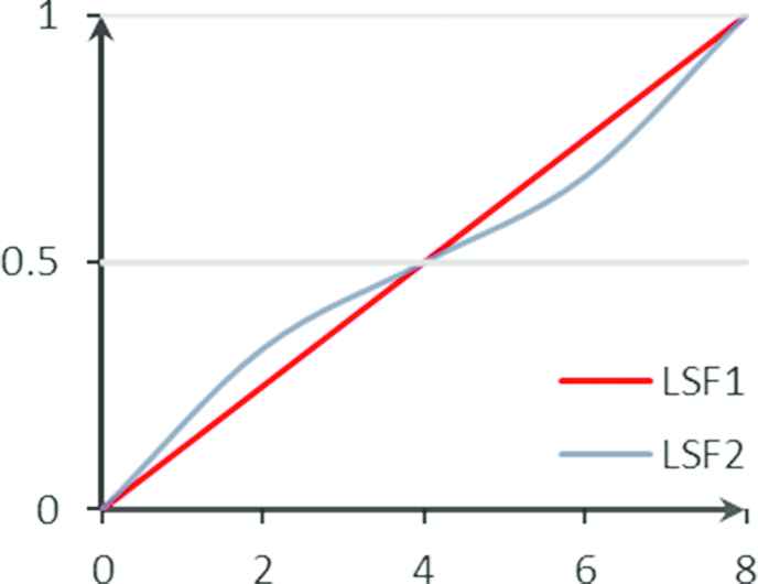
Illustration of linguistic scale function 1 (LSF1), LSF2.
By using bidirectional geometric growth, an LSF2 can better reflect the psychological processes of the DMs when judging the good and bad characteristics of the different criteria values. Although the ranking result of SVN–TODIM method based on LSF2s are closer to the proposed method, the LNNs can represent more complex information by using LTSs than by using SVNs, especially in a qualitative decision-making environment. All these examples show that the proposed method-based new SFs with LNNs is more flexible and more innovative.
It can be seen from the above comparisons and analysis that the proposed method based on the new SFs of LNNs has an advantage over the SVN–TODIM method that is described in Reference [33] and the TOPSIS method that is described in Reference [32] because it takes full advantage of the evaluation information by the LNNs and can consider the DMs’ psychological behavior by comparing evaluation values.
7. CONCLUSION
As an effective linguistic expression, an LNN makes the best use of the advantages of the LVs and SVNNs that describe uncertain and inconsistent information by using LVs. Then, the TODIM method is a suitable and reasonable tool for MCGDM problems that can consider the DMs’ psychological behavior. Therefore, it is a good idea to apply the TODIM method under a linguistic neutrosophic environment. To better reflect the risk preferences of the DMs facing a gain or a loss, we improved the SF of the LNNs that can effectively compare LNNs without the assistance of an accuracy function. Based on a subjective weight model and the objective weight model, we developed a combined weight model that not only considers the DMs’ preferences but also makes full use of the evaluation information. Consequently, an improved TODIM method based on the revised SF and the combined weight model is proposed. Then, we demonstrated the procedures of the proposed method and validated the effectiveness and advantages of the proposed method by comparison with other methods found in References [18, 32, 33]. The main contribution of this paper is a new approach for MCGDM problems with LNNs that enriches the existing research theories of LNNs. For our future studies, we will focus on the information preferences of the DMs in the form of the LNNs and we would like to develop potential applications of the proposed method in different domains, such as facility location, quality assessment, personnel recruitment, and so on.
ACKNOWLEDGMENTS
This paper is supported by the National Natural Science Foundation of China (Nos. 71771140 and 71471172), the Special Funds of Taishan Scholars Project of Shandong Province (No. ts201511045).
REFERENCES
Cite this article
TY  - JOUR
AU  - Peide Liu
AU  - Xinli You
PY  - 2019
DA  - 2019/04/23
TI  - Improved TODIM Method Based on Linguistic Neutrosophic Numbers for Multicriteria Group Decision-Making
JO  - International Journal of Computational Intelligence Systems
SP  - 544
EP  - 556
VL  - 12
IS  - 2
SN  - 1875-6883
UR  - https://doi.org/10.2991/ijcis.d.190412.001
DO  - 10.2991/ijcis.d.190412.001
ID  - Liu2019
ER  -