
Rough Number–Based Three-Way Group Decisions and Application in Influenza Emergency Management
- DOI
- 10.2991/ijcis.d.190420.001How to use a DOI?
- Keywords
- Three-way decisions; Group decision-making; Rough numbers; Risk preference
- Abstract
Group decision-making can effectively deal with complex decision problems in reality and takes important research status in the field of decision-making. In recent years, three-way decision has been a hot topic in the field of uncertain decision-making, so the models of three-way decision under group environment have become a new direction and problem in decision-making research. Based on the subjectivity and uncertainty of the group judgment, this paper adopts the rough number method to objectively and effectively integrate the group information so as to establish rough number–based three-way decision models. First of all, we use rough numbers to transfer loss functions of individuals into a rough number–based gathering loss function, and verify the rough number–based loss function meets the general characteristics of general loss functions. Then from the perspectives of optimism, pessimism, risk preference of decision-makers, and directly operation of rough numbers, we explore the calculation of thresholds and the acquisition method of three-way rules, and then establish rough number–based three-way group decision models. Finally, influenza emergency management is introduced to verify the effectiveness and advancement of the novel method.
- Copyright
- © 2019 The Authors. Published by Atlantis Press SARL.
- Open Access
- This is an open access article distributed under the CC BY-NC 4.0 license (http://creativecommons.org/licenses/by-nc/4.0/).
1. INTRODUCTION
Three-way decision-making is a decision-making theory developed on the basis of the decision-theoretic rough set (DTRS). Ever since its introduction by the Canadian scholar Yao in 2009, it has attracted wide attention in academia. To provide a reasonable semantic explanation for the three regions divided by the upper and lower approximate sets in the rough set theory, Yao corresponded the positive, boundary, and negative domains in the rough set model with three decision-making results: acceptance, noncommitment, and rejection [1,2]. The author also expanded the traditional two-way decision-making model with only two outputs (acceptance and rejection) into a three-way model, which more accurately describes the characteristics of human thinking and behavior. Three-way decision-making frequently occurs in real life. For example, a manuscript review by experts based on two-way decision-making leads to one of two results: acceptance or rejection. In the actual review process, however, most manuscripts cannot be directly categorized into the above two results. Instead, a third decision-making result, noncommitment, is selected, in which further revision required. This gives rise to a three-way decision-making problem. Three-way decision-making is proposed based on the idea of the DTRS. The DTRS starts with Bayes' theorem and uses loss functions to describe the risks in decision-making. It selects the decision-making behavior with the minimum risk in response to the expected risks of three-way decision-making results, namely, acceptance, delayed decision-making, and rejection. Two important elements in the DTRS are the conditional probability and the threshold. The final decision-making behavior is determined by comparing their magnitude. Three-way decision-making has already been widely applied in many areas, such as investment decision-making [3,4,5], conflict analysis [6], face recognition [7,8], email filtering [9], medical diagnosis [10,11], and recommendation systems [12,13].
The greatest advantage of three-way decision-making over traditional decision-making methods is that it can reduce the loss caused by incorrect classification. There are many decision-making problems in real life. Once an incorrect decision is made, the resulting loss may be immeasurable, especially for emergencies. In complicated decision-making situations with short decision-making time, incorrect decision-making often results in a series of adverse consequences. The management of an influenza epidemic situation is a typical emergency management event. In recent years, a variety of influenza viruses have caused outbreaks one after another, for example, H1N1. There are both correct and incorrect judgments on influenza epidemic situations. A correct judgment can control the development of the epidemic situation, whereas an incorrect judgment can easily lead to a large-scale influenza outbreak or social disorder. Figure 1 shows four results caused by different decisions aiming at whether the influenza outbreak or not. Suppose there are several influenza cases in a certain city, and the health department needs to determine whether or not this is a harbinger of an influenza outbreak based on the current situation and whether or not preventive measures should be implemented, such as issuing influenza warnings or deploying isolation procedures. The quadrant (ii) and (iv) depict the correct decisions, where quadrant (ii) represents that the city is suffering the influenza and the government decides to take protection actions to reduce the losses, and quadrant (iv) represents that no influenza outbreaks in this city and the government takes no action. While the quadrant (i) and (iii) demonstrate the mistakes in decision-making: the quadrant (iii) shows the type I error (rejection of a true null hypothesis), which means it is currently at the stage of an influenza outbreak, but the government has not taken any measures, which will result in spreading of influenza and more cases; the quadrant (i) shows the type II error (acceptance of a false null hypothesis), meaning that the current situation will not cause an influenza outbreak, but the government takes actions like issuing influenza warnings and deploying isolation procedures, which will cause the general public panic and disturb the normal functioning of society, and even social chaos. In particular, with the current development of the Internet, information spreads much faster, easily leading to the spread of rumors. For instance, a few years ago, a prevailing rumor that H7N9 would outbreak in China caused people to rush out and buy Banlangen (the root of Isatis indigotica) and white vinegar. This resulted in social unrest and consequences even worse than the influenza outbreak itself. Therefore, there is a new research approach in which three-way decision-making is used to cope with practical decision-making problems, especially emergency management problems.
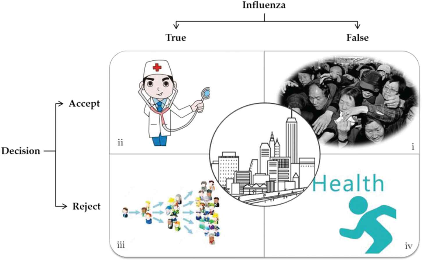
Decision results for influenza emergency management.
As an essential element of three-way decisions, the determination of loss functions is a key procedure and has attracted most attention. It is almost impossible to obtain exact losses by instruments or technologies, so in most realistic problems, losses need to be determined by related experts. For example, the losses of medical diagnosis problems need to be determined by doctors according to their knowledge and experience. While it is undeniable that there exists uncertainty and subjectivity in experts' opinions, therefore, many researches considered uncertainty and constructed three-way decision-making models based on different expression forms of losses. Liu and Liang described the loss using the interval number and constructed DTRS models based on the interval number [14,15], which has provided ideas for later research on three-way decision-making on uncertainty information. Liu introduced randomness into the loss function and constructed a random three-way decision-making model, the relevant characteristics of which were explored based on uniform distributions and normal distributions separately [5]. Subsequently, Liang et al. expanded the three-way decision-making model to fuzzy cases in which the loss function is expressed in the forms of triangular fuzzy numbers [16], intuitionistic fuzzy numbers [17], hesitant fuzzy numbers [18], and other data types. Corresponding three-way decision-making models were constructed, and the threshold calculation method was given to make the optimal decision. Liang et al. used linguistic terms to evaluate the selection and constructed a linguistic three-way decision-making method [19]. Three-way model was introduced into information table with order relation, and then the ordered three-way decisions were constructed as well as the algorithm [20].
As the complexity of decision environment and the limitation of human cognition, opinion of single decision-maker could not describe losses correctly. Therefore, to express losses in a comprehensive way, a few researches have introduced group decision-making approaches to three-way decisions. In traditional group decision-making methods, different aggregating approaches have been discussed according to different forms of evaluating values, some of which have been applied into three-way decision problems. By using the idea of granular computing, Liang aggregated and expressed the loss function as interval numbers and thus established a three-way group decision-making model [21]. After that, Liang expanded group decision-making to a loss function of linguistic value and constructed a three-way group decision-making model based on linguistic evaluation information [19]. Sun constructed a three-way group decision-making model based on a multigranularity fuzzy DTRS [22]. Liu constructed a three-way group decision-making model by taking the decision-makers' attitudes and preferences into consideration and integrating these with the prospect theory [23]. By aggregating group information, an aggregated loss function can be found, and then the thresholds. The conditional probability is always observed by historical experience, and then decision rules can be obtained through comparing conditional probability and thresholds.
Although there exist some studies about three-way group decision-making models, the research for group decision in three-way models is still in the exploratory stage. According to the discussion above, all the approaches for group aggregation in three-way decisions ignores the intrinsic links among evaluation information from decision-makers. Zhai proposed a novel approach, the rough number, which is proposed to quantify experts' cognition based on rough set theory, and can be used for group aggregation by considering the intrinsic relationship among decision-makers [24,25]. Therefore, this paper intends to discuss three-way group decision-making models in the novel perspective of rough number. A rough number is represented as an interval numbers formed by upper and lower limits. It does not require any prior information, but it is determined completely based on the original data. The rough number method can comprehensively take the evaluations from all experts and integrate decisions made by individual experts into a group decision to ensure the objectivity and accuracy of the data and results. The rough number method was originally applied in the development of new products initiated by quality function. Zhai used the rough number method to effectively compile subjective evaluations and judgments of consumers and integrated individual evaluation values into rough numbers, which were then employed for data mining and decision-making [25]. Subsequently, many scholars have integrated the rough number method with the multicriteria decision-making method and have obtained decision-making models, such as rough number AHP (analytic hierarchy process); [26], rough number BWM (best-worst method); [27], and rough number TOPSIS (technique for order preference by similarity to an ideal solution) [28]. Since its introduction, the rough number method has been widely used as an effective way of assembling group information.
Therefore, the aim of this research is to construct a novel three-way group decision-making model based on rough numbers, which can aggregate multiple experts' information in a reasonable way, obtain rough loss functions, and receive more effective three-way rules, and then be used in influenza emergency management problems. The remainder of this paper is organized as follows. Section 2 lists some basic concepts of three-way decisions with DTRSs and rough numbers. Section 3 proposes the construction process of group loss functions based on rough numbers. In section 4, according to group loss functions, we discuss the acquisition methods of three-way rules from four different perspectives. To illustrate the application in influenza emergency management, section 5 presents a practical case in China and discuss the effectiveness of the model. Section 6 concludes this paper and outlines the future work.
2. PRELIMINARIES
This section is composed of two subsections to review some preliminaries about three-way decisions with DTRSs and the method of rough numbers.
2.1. Three-Way Decisions Based on DTRSs
To illustrate the principle of rough sets, Pawlak defined the approximation space as
The PRSs divide the universe
In particular, the models can be degenerated to traditional two-way decisions when
In order to give semantic interpretations of the thresholds and three regions in PRSs, Yao proposed DTRSs with the aid of Bayesian theory [29]. A DTRS model is composed of two states and three actions, which can be seen in Table 1. The set of states can be expressed as
The loss functions.
For
According to Bayesian theory, the best decision is the one with minimum cost, so decision rules can be indicated as follows:
Since
Suppose there exists an assumption
On the contrary, if the assumption is
The rules (P″)-(N″) and (P‴)-(N‴) indicate that three-way decisions must satisfy the condition Equation (16) or
2.2. Rough Numbers
Inspired by rough set theory, rough number is firstly proposed by Zhai [24] in order to handle subjective preferences of customers in quality function deployment. Similar to the notion of approximates in rough sets, a rough number is constructed by lower and upper limits, which determine a rough boundary interval to characterize imprecise information. Rough numbers merely depend on original data without any prior knowledge, so they can capture the experts' real perception effectively, and aggregate every individual's preference into an objective and consistent group judgement. In this subsection, we review some basic concepts of rough numbers.
Suppose
Then
To compare the values of rough numbers, Zhai proposed the ranking rules [25]. For any two rough numbers
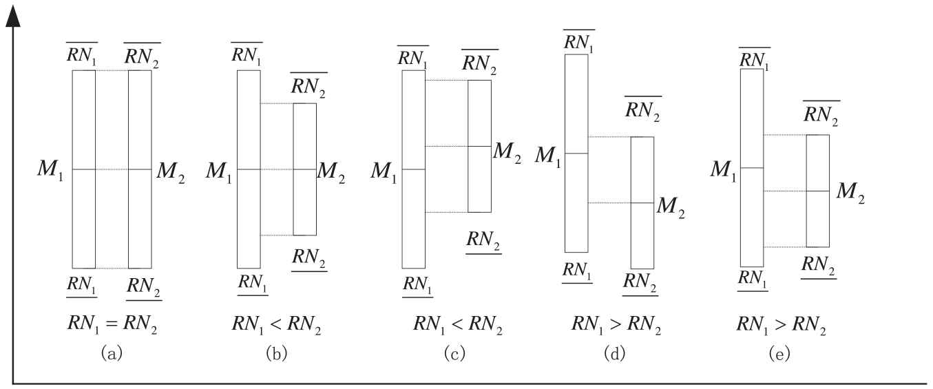
Ranking rules for rough numbers.
For an easy-to-operate purpose, we illustrate the ranking rules in an accurate mathematical linguistics rather than a graphical representation. Denote
If
If
If
if
if
if
Where
Based on the construction of
For a convenient expression,
Rough numbers are similar to interval numbers in form, so with the aid of arithmetic operations of interval analysis, Zhai proposed the operations of rough numbers [24]. Suppose
3. THE AGGREGATION OF LOSS FUNCTIONS BASED ON ROUGH NUMBERS
3.1. Description of Three-Way Group Decision-Making
The most important issue of the three-way decision-making model is the determination of the loss function. For losses caused by incorrect classification, researchers usually use subjective experiences and evaluation by relevant experts to determine the loss values. While due to the lack of knowledge and experience, and the limitation of individual subjective knowledge, individuals find it difficult to have systematic and comprehensive understanding of decision-making problems. Therefore, group decision-making has become an important approach in the field. In a group decision-making perspective,
The loss function of
3.2. Rough Number–Based Loss Functions
By integrating the evaluation information from
The results of experts' evaluation.
For any
Therefore, the rough number–based evaluation values of
By using Equations (20) and (21), aggregated loss function can be obtained and represented as
Rough loss function.
Therefore, the aggregated rough loss
According to the discussion in section 2, three-way decisions must satisfy the conditions
Theorem 1.
If for any
Proof.
Firstly, we prove
It is obvious that there are
For
According to the discussion, we can prove
So the theorem has been proved.
Theorem 1 illustrates that the aggregated loss functions based on rough numbers still satisfy the conditions in classical three-way decisions, which guarantee the validity and reasonability of the further research.
4. THREE-WAY GROUP DECISION MODELS BASED ON ROUGH LOSS FUNCTIONS
By using rough numbers to aggregate the information of decision-makers, the rough loss function, as shown in Table 4, has been obtained, wherein the losses are expressed as rough numbers. In this section, we intend to explore how thresholds, rules, and classifications are obtained in group three-way decisions based on rough loss functions. In consideration of the risk preferences of decision-makers, this section explores decision-making strategies from three perspectives, namely optimism, pessimism, and risk preference coefficient. Then a direct method to acquire the threshold and three-way rule is given based on the algorithm of rough numbers without taking into account the decision-maker's risk preference.
4.1. Three-Way Group Decision Models with Risk Preference
4.1.1. Model 1: An optimistic perspective
The optimistic perspective refers to a situation in which decision-makers believe that the loss caused by incorrect classification is the smallest. Therefore, only the lower limits of rough losses
Optimistic loss function.
According to the acquisition procedure of three-way decision rules, the expected losses of different actions
According to Bayesian theory, the optimistic decision rules can be indicated as follows:
Based on the properties shown in Theorem 1, we can obtain that
Example 1.
Suppose in a group decision-making problem, we have obtained the aggregated rough loss function, and the losses of misclassifications are expressed as
4.1.2. Model 2: A pessimistic perspective
The pessimistic perspective means that the decision-maker believes that the loss caused by incorrect classification is the greatest. Hence, for the rough number loss function, only the upper limits of the rough losses
Pessimistic loss function.
Based on the acquisition procedure of three-way decision rules, the expected losses when choosing different actions
According to Bayesian theory, the pessimistic decision rules can be denoted as follows:
From Theorem 1, we can obtain that there exist
Example 2.
Continue the Example 1. Based on the pessimistic viewpoint, we determine the upper limits of rough numbers as the final losses, which can be written as
4.1.3. Model 3: Risk preference coefficient
For many practical problems, the risk preferences of decision-makers are neither pessimistic nor optimistic, and they may be between the two instead. In such a case, a coefficient can be employed to describe the risk preference so that the losses in three-way decisions can be determined.
Definition 1.
For any rough number
From Definition 1, we know that
With the risk preference coefficient, it is possible to determine the loss function expressed using real numbers, which are shown in Table 7.
Loss function based on
Where
Based on the loss function derived from risk preference coefficient, the expected losses of different actions
According to Bayesian theory, the decision rules under risk preference coefficient model can be expressed as follows:
Theorem 1 illustrates that
Where
Example 3.
We continue to use the data in Example 1. Denote the risk preference coefficient as
4.2. Three-Way Group Decision Model Based on Rough Numbers
The models discussed above are all based on the viewpoint that converting rough numbers into real numbers. And in this section we intend to solve rough-number based three-way decisions in a direct way. According to the rough loss function shown in Table 4, we can obtain three-way decision rules by utilizing the arithmetic operations and ranking rules of rough numbers. The specific procedure is shown as follows.
Based on rough loss function in Table 4, the expected losses of different actions ai can be denoted as
According to the arithmetic operations of rough numbers, we can obtain the expected rough losses as
Simplify the decision rules based on Bayesian theory and we can get
Where
If
For the two cases: (1) if
It is worth noting that, in Equation (55), whether
| Conditions | Subconditions | Sub-subconditions | Results | No. |
|---|---|---|---|---|
| — | — | (a) | ||
| — | — | (b) | ||
| — | — | (c) | ||
| (d) | ||||
| (e) | ||||
| (f) | ||||
| (g) | ||||
| (h) | ||||
| (i) | ||||
| (j) | ||||
| (k) | ||||
| (l) | ||||
| (m) | ||||
| (n) | ||||
| (o) | ||||
| — | (p) | |||
| — | (q) | |||
| — | (r) |
Rough three-way decision rules.
In Table 8, three-way decision rules can be classified to three cases: (1) the normal case, where there is
Rules in normal case
In this case,
Where
Rules in extreme case I
In this case there exists
Suppose there are
if there is
for
for
if there is
for
for
Similarly, the cases when
Rules in extreme case II
In this case, there is
In conclusion, 18 three-way decision rules derived from rough loss functions can be obtained, as shown in Table 8.
Example 4.
We discuss the problem in Example 1 by using the direct model proposed in this subsection. The expected rough losses can be calculated as
According to Equations (56–58), we can obtain the values of three thresholds, which are denoted as
5. AN APPLICATION IN INFLUENZA EMERGENCY MANAGEMENT
5.1. Problem Description
As an important practical issue in human society, influenza emergency management is discussed in this section by using rough number–based three-way group decisions. A city in China is suffering from a suspected influenza outbreak. The health department of the city plans to isolate regions where influenza cases have been diagnosed, and takes no preventive measures in regions where there is no influenza outbreak. Based on the judgment on the influenza epidemic, two states
It is difficult to accurately calculate losses caused by incorrect classification of influenza epidemic situations. Therefore, five experts in influenza emergency management are selected to form a decision-making group
| 2 | 13 | 20 | 14 | 7 | 2 | |
| 3 | 10 | 21 | 13 | 6 | 1 | |
| 3 | 8 | 20 | 15 | 5 | 2 | |
| 4 | 7 | 19 | 13 | 7 | 3 | |
| 2 | 6 | 28 | 17 | 8 | 2 |
Results of experts' evaluation.
Based on the constructing process of rough numbers shown in Equations (17–21), the evaluation values of decision group can be aggregated to rough losses, as shown in Table 10.
Rough loss function.
5.2. Three-Way Decisions of Influenza Emergency Management
According to the four models proposed in Section 4, that is to say, the optimistic model, the pessimistic model, the risk preference coefficient model, and the rough model, we can obtain different decision results under various environments.
According to model 1 based on the optimistic perspective, the optimistic loss function can be denoted as Table 11. And by using Equations (29–31), we can calculate the values of thresholds as
According to model 2 based on the pessimistic perspective, the pessimistic loss function can be denoted as Table 12. By using Equations (35–37), we can obtain the values of thresholds as
According to model 3 based on the risk preference coefficient perspective, we can obtain the loss function based on
According to the direct rough model proposed in Section 4.2, we can calculate the values of thresholds by using Equations (56–58) based on the data in Table 10, and obtain that
The final results derived from four models can be depicted in Table 14 and Figure 4.
| 2.36 | 13.50 | |
| 7.21 | 5.92 | |
| 20.15 | 1.65 |
Optimistic loss function.
| 3.25 | 15.43 | |
| 10.63 | 7.25 | |
| 23.88 | 2.35 |
Pessimistic loss function.
| 2.98 | 14.85 | |
| 9.60 | 6.85 | |
| 22.76 | 2.14 |
Loss function based on
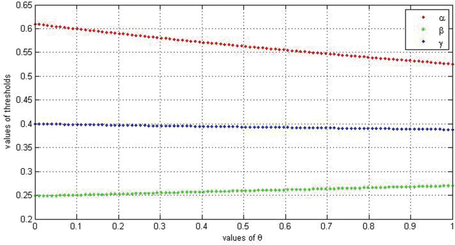
The thresholds values with different values of
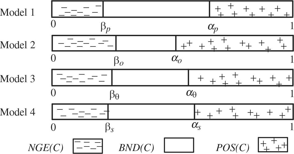
Three-way decisions based on different models.
The above four results have different effects on the determination of the three-way decision-making rules. All results are summarized in Table 14. Table 14 shows that regardless of which decision-making method is selected, the final classifications of
| Administrative Regions | Conditional Probabilities | Decision Results | |||
|---|---|---|---|---|---|
| Model 1 | Model 2 | Model 3 | Model 4 | ||
| 0.54 | |||||
| 0.21 | |||||
| 0.32 | |||||
| 0.65 | |||||
| 0.58 | |||||
| 0.26 | |||||
| 0.25 | |||||
| 0.57 | |||||
Results of decision-making.
5.3. Comparison and Discussion
According to previous research, for three-way decision-making models with multiple decision-makers, methods such as taking the maximum value, the minimum value, and the weighted average can be used to aggregate the group information, and the group loss function can be obtained. Then the final three-way decision rules are obtained by using the three-way decision-making process. Here the results obtained by the weighted average method and the three-way group decision-making model proposed in literature [21] were selected and compared with those obtained using the methods in this study, which are shown in Tables 15 and 16.
| Methods | Thresholds | ||
|---|---|---|---|
| Weighted average method | 0.565 | 0.265 | 0.397 |
| Method proposed by Liang [21] | 0.571 | 0.218 | 0.381 |
| Model 1 | 0.610 | 0.248 | 0.400 |
| Model 2 | 0.526 | 0.270 | 0.388 |
| Model 3 | 0.547 | 0.264 | 0.391 |
| Model 4 | 0.563 | 0.259 | 0.394 |
Comparison of thresholds.
| Methods | Classification | ||
|---|---|---|---|
| POS(C) | BND(C) | NEG(C) | |
| Weighted average method | {x4, x5, x8} | {x1, x3} | {x2, x6, x7} |
| Method proposed by Liang [21] | {x4, x5 } | {x1, x3, x6, x7, x8} | {x2} |
| Model 1 | {x4 } | {x1, x3, x5, x6, x7, x8} | {x2} |
| Model 2 | {x1, x4, x5, x8} | {x3} | {x2, x6, x7} |
| Model 3 | {x4, x5, x8} | {x1, x3} | {x2, x6, x7} |
| Model 4 | {x4, x5, x8} | {x1, x3, x6} | {x2, x7} |
Comparison of classifications.
Table 15 illustrates the values of thresholds obtained by different methods. The values are various according to the selection of methods, but all the thresholds of each method satisfy
The specific advantages of models in this paper are summarized as follows:
By using the rough number method to aggregate group information, it is possible to take advantage of the rough number method and to fully consider and explore the intrinsic relations among all information in the same evaluation category, which can effectively eliminate the effect of abnormal evaluating values.
The rough number method can reflect the objectivity of the rough set theory. No subjective prior knowledge is required, and only the intrinsic relations among information should be taken into consideration. Thus, the objectivity of the aggregation of group information is guaranteed, and the decision-making rules obtained are also more reliable.
Three-way group decision-making models based on rough numbers can utilize different decision-making modes. For example, the risk preferences of decision-makers in a decision-making situation can be taken into account, or the rough number calculation method can be employed when risk preferences are not considered. Decision-makers could select different three-way group decision-making models in various environments, which can result in decision-making rules that better address problems in real life and can offer greater flexibility.
6. CONCLUSIONS
Group decision-making involving multiple decision-makers is an important way to solve practical decision-making problems. This paper explored the integration of group decision-making with three-way decision-making models and their application. To handle the problem of group information aggregation in the process of group decision-making, the rough number method is adopted. Since the rough number method is objective and systematic, the estimation of the loss functions by all individuals in the group are aggregated to construct the rough number loss function and thus to describe the evaluation information of the group. In the construction stage of the three-way decision-making model, based on whether or not the decision-maker's risk preference should be taken into account, the optimistic method, the pessimistic method, the risk preference coefficient method, and the rough number calculation method were constructed respectively to examine the threshold calculation and the rule acquisition in three-way decision-making models. Finally, the three-way group decision-making model constructed in this paper was applied to an influenza emergency management problem to make the optimal decision with the lowest loss caused by errors. The three-way group decision-making model based on the rough number method is able to effectively aggregate the estimation of the loss function by the decision-making group to reflect the overall preference of the decision-making group and to choose different decision-making modes according to the actual problems to obtain decision-making rules. In future studies, three-way group decision-making models with group uncertain information, such as interval numbers and fuzzy numbers, will be further explored. Meanwhile, other emergency management problems will be selected for application.
ACKNOWLEDGMENTS
This paper is supported by the National Natural Science Foundation of China (Nos. 71771140 and 71471172), the Special Funds of Taishan Scholars Project of Shandong Province (No. ts201511045), and the Humanities and Social Sciences Research Project of Ministry of Education of China (No. 19YJC630059).
REFERENCES
Cite this article
TY  - JOUR
AU  - Fan Jia
AU  - Peide Liu
PY  - 2019
DA  - 2019/04/26
TI  - Rough Number–Based Three-Way Group Decisions and Application in Influenza Emergency Management
JO  - International Journal of Computational Intelligence Systems
SP  - 557
EP  - 570
VL  - 12
IS  - 2
SN  - 1875-6883
UR  - https://doi.org/10.2991/ijcis.d.190420.001
DO  - 10.2991/ijcis.d.190420.001
ID  - Jia2019
ER  -