
Using Multi-Conditional Minimum Thresholds in Temporal Fuzzy Utility Mining
- DOI
- 10.2991/ijcis.d.190426.001How to use a DOI?
- Keywords
- Fuzzy data mining; fuzzy set; Temporal fuzzy utility mining; Multiple thresholds; Extended two-phase model
- Abstract
In the field of fuzzy utility mining, the characteristics of transaction time have been a widely studied topic in data mining. However, using a single-conditional threshold for all items does not suffice to reflect the true properties of items. This paper, therefore, proposes a multi-conditional minimum threshold approach which considers the temporal behavior, the importance in items, and the usage of linguistic terms to mine high temporal fuzzy utility itemsets. The multi-conditional minimum thresholds are utilized to assist users in deciding appropriate standards for itemsets in mining when its contained items have different importance. An extended two-phase model and a corresponding mining approach are designed to handle the temporal fuzzy utility mining problem with the multi-conditional minimum thresholds. Finally, the results from the experimental evaluation show the effectiveness of the proposed approach under different settings.
- Copyright
- © 2019 The Authors. Published by Atlantis Press SARL.
- Open Access
- This is an open access article distributed under the CC BY-NC 4.0 license (http://creativecommons.org/licenses/by-nc/4.0/).
1. INTRODUCTION
Discovering knowledge discovery in data mining have been widely studied due to its wide applications. Frequent patterns found by association-rule mining is one of the fundamental research issues, as it can be used to identify implicit relationships among items in a database [1–3]. One drawback of association-rule mining, however, is that we cannot take for granted that the quantity of an item is binary. Besides, it cannot consider the profit of an item as an essential factor, either. As such, mining frequent itemsets are easy, in contrast to finding high-utility itemsets with the quantitative information and unit profit. Thus the utility mining strategy [4] was proposed, which considers both the sold quantities of items and their corresponding unit profits in transactions for recognizing the actual utility values of itemsets and thus discovering high-utility itemsets from a transaction database. Most of the related approaches were designed to improve the execution efficiency [5–9], to find the items with negative profits [10], to consider the on-shelf periods of the items [11–13], or to process the dynamic update of the datasets [14,15]. However, quantitative values are still not easily understood by decision-makers.
To resolve the problem, fuzzy sets provided a good solution, and thus fuzzy utility mining strategy [16,17] was proposed. Transforming quantitative information in each transaction to implied fuzzy terms by using the membership functions of each item, with the fuzzy intersection operator of fuzzy sets, users can easily comprehend the implication of quantity.
However, fuzzy utility mining has difficulty in maintaining the downward-closure property which is the main principle for association-rule mining to prune candidate itemsets efficiently. Lan et al. presented a fuzzy utility function and adopted the minimum operator for the intersection [17]. Besides, they propose an effective model with fuzzy utility upper bounds to prune unpromising candidates early in fuzzy utility mining. Going on the above concept, the late-on-shelf items in a supermarket may be obscured in fuzzy utility mining. Therefore, temporal fuzzy utility mining [18] was proposed to consider the first on-shelf time of an item to find more relevant patterns. Most works in fuzzy utility mining have been proposed to handle various applications but use only a single-conditional measurement for determining high fuzzy utility itemsets [16–18].
Nevertheless, a single-conditional measurement [9–11,16] may not accurately reflect the properties of items and itemsets in real applications, such as the difference in significance between emerging items and aged ones. In the past, several algorithms considering multiple-conditional measurements for association-rule mining [19–23], fuzzy association-rule mining [24,25], utility mining [26], and sequential pattern mining [27] have been studied. In these approaches, each item can be assigned an individual threshold.
According to the above reasons, in this paper, we consider the temporal fuzzy utility mining problem with multi-conditional minimum thresholds (TFUMPmmt). In the problem, the given minimum thresholds depend on the items. A mechanism is then designed to decide the minimum thresholds of itemsets based on the fuzzy operators. To avoid information loss, an extended two-phase model is provided to keep the downward-closure property for TFUMPmmt, and a TPM (Two-Phase Multi-conditional algorithm for temporal fuzzy utility mining) algorithm is proposed to solve it. At last, experimental results are given to compare the efficiency and effectiveness of the proposed approach and that for the temporal fuzzy utility mining problem with single-conditional minimum threshold (TFUMPsmt).
2. RELATED WORKS
The association-rule mining, such as the Apriori approach proposed by Agrawal et al. [1,2] and the FP-growth presented by Han et al. [28], focuses on binary mining to reveal the co-occurrence relationship of items but cannot discover itemsets with high profit. Products with high profit but low frequency may not be found in mining. The utility model, proposed by Yao et al. [4], then keeps the quantitative value of items and their profits to solve the disadvantage. Besides, Chan et al. [29] proposed the topic of utility mining, which considered not only quantities of items in a transaction but also profits of items in a database, to find itemsets with high utility values. However, the high-utility itemsets discovered contain just items without quantitative information and are difficult for users to comprehend the quantitative relationship of the items.
Fuzzy quantifiers can represent fuzzy approximation to the implicit meaning of facts [30,31]. For example, “two oranges” in a quantitative sentence can be treated as a “low” amount label for the semantic meaning needed by decision-makers. Thus, the methods of fuzzy utility mining were designed to capture the explicit meaning of the quantity sold. For example, Lan et al. [17] presented a framework to discover high fuzzy utility itemsets by adopting the fuzzy concepts to convert the quantity information in a quantitative transactional dataset into fuzzy regions. Wang et al. [16] also defined fuzzy utility mining as the problem of identifying linguistic itemsets taking into account both whole (i.e., three apples) and fractional (i.e., 2.1 pounds) quantities.
The methods mentioned above did not consider the temporal factor of the items while discussing high-utility or fuzzy utility itemsets. Because of this, short-sale or time-limited items in a supermarket may be obscured in mining. For example, during summer or winter vacations, supermarkets use different sale strategies to promote unfixed products. However, if all the products on shelves are viewed as being of the same time, it is difficult to explore the various combinations of products effectively, especially in short-sale or time-limited situations. To overcome the limitation, Huang et al. [18] in 2017 introduced fuzzy utility mining with consideration of transactional time (TFUM). But they only use a single minimum threshold to get high temporal fuzzy utility itemsets (HTFUIs).
The use of a single-conditional threshold in mining has largely been applied in utility mining [4,7,12,13], incremental utility mining [15], and fuzzy utility mining [17,18]. Existing approaches employ the threshold for all items as a measuring standard to mine desired itemsets. However, considering all items of the same importance does not reflect real-world practice. Thus, the threshold requirement should depend on the items to get better effects. For example, people will consider the utility of emerging items and aged ones under different criteria. An emerging item may not currently get much profit, but it may have a high potential to earn much money in the future. Hence, using a minimum fuzzy utility threshold for all items in fuzzy utility mining is not a fair measurement. Although taking into account multiple item thresholds better reflects real-world needs, it is also more challenging.
3. MINING TEMPORAL FUZZY UTILITY ITEMSETS WITH MULTI-CONDITIONAL MINIMUM THRESHOLDS
3.1. The Concept of the Proposed TPM Method
The proposed method mines HTFUIs under multi-conditional minimum thresholds. Figure 1 shows the execution process of the proposed TPM method.
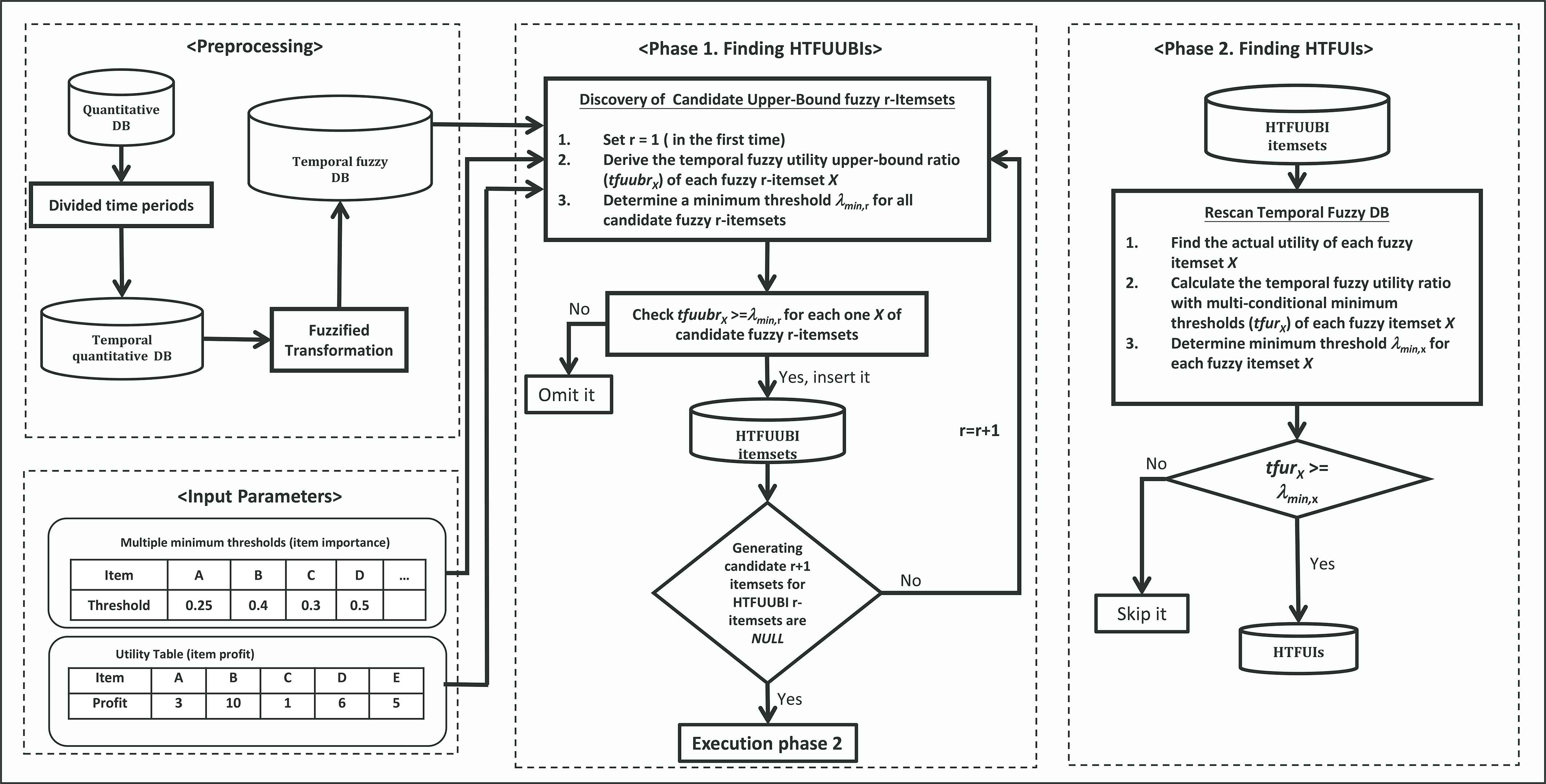
The overall mining process of the two-phase multi-conditional (TPM) algorithm.
In Figure 1, the <Preprocessing> dotted box contains the parameters of the proposed approach and the fuzzified process of the transaction data. First, a quantitative database is transformed into a corresponding temporal quantitative database by time periods, which is then converted into the temporal fuzzy database by fuzzy transformation. The <Input parameters> dotted box includes a utility table storing the profit of each item and a set of multiple minimum thresholds with items. After the preprocessing steps are conducted, the proposed mining method has two main phases. In the first phase, the algorithm determines the high upper-bound itemsets which satisfy the upper-bound ratio. Then in the second phase, the upper-bound itemsets derived in the first phase are further checked to find their actual fuzzy utility values. The fuzzy itemsets with their actual fuzzy utility values larger than or equal to the corresponding thresholds are output as the results. In this way, the proposed method can find the complete set of HTFUIs satisfying the multi-conditional minimum constraints.
3.2. Formal Problem Definition
Let P = {P1, P2, …, Pm}, where m represents the number of time periods and Pi represents the i-th time period, be a set of adjacent disjoint time periods with a d ∈ esignated time granularity. Given a set I of n distinct items {i1, i2, …, in}, a quantitative transaction database is a set of transactions represented as QTD = {Qtrans1, Qtrans2, …, Qtransy, …, Qtransz}, in which each transaction QtransyQTD
| Period | TID | A | B | C | D | E | F | G |
|---|---|---|---|---|---|---|---|---|
| P1 | Qtrans1 | 2 | 0 | 2 | 3 | 5 | 1 | 0 |
| Qtrans2 | 0 | 1 | 25 | 0 | 0 | 0 | 0 | |
| Qtrans3 | 0 | 0 | 0 | 0 | 10 | 1 | 0 | |
| Qtrans4 | 0 | 1 | 12 | 0 | 0 | 0 | 0 | |
| P2 | Qtrans5 | 4 | 0 | 8 | 0 | 10 | 0 | 0 |
| Qtrans6 | 0 | 0 | 4 | 3 | 0 | 1 | 0 | |
| Qtrans7 | 0 | 0 | 2 | 3 | 0 | 0 | 0 | |
| P3 | Qtrans8 | 6 | 2 | 0 | 0 | 10 | 3 | 0 |
| Qtrans9 | 4 | 0 | 0 | 4 | 0 | 0 | 3 | |
| Qtrans10 | 0 | 0 | 4 | 0 | 10 | 0 | 0 |
An example of a temporal quantitative dataset.
It is used throughout this work to help explain the definitions. In the dataset, there are 10 transactions which consist of 7 items in total, denoted from A to G. There are three time periods, P1 to P3, in this example. Table 2 represents the profit table and Table 3 shows the minimum fuzzy utility thresholds of all the items. The membership functions of each item are shown in Figure 2.
| Item | Profit |
|---|---|
| A | 3 |
| B | 10 |
| C | 1 |
| D | 6 |
| E | 5 |
| F | 2 |
| G | 20 |
The profit table.
| Item | Minimum Threshold |
|---|---|
| A | 0.25 |
| B | 0.4 |
| C | 0.3 |
| D | 0.5 |
| E | 0.25 |
| F | 0.25 |
| G | 0.3 |
The minimum thresholds of all the items.

Membership functions of the items in Table 1.
To explain the proposed TPM algorithm clearly, we offer the formal definitions for TFUMPmmt as follows: Let a fuzzy region of an item is called a fuzzy item, and a fuzzy itemset is composed of one or more fuzzy items with the condition that no two fuzzy items are formed from an identical item. For example, A.Low, A.Middle, and A.High are three fuzzy items derived from the item A, and {A.Low, B.High} is a fuzzy itemset. Note that {A.Low, A.High} cannot be a fuzzy itemset since both of the fuzzy items come from the same item A.
1st Definition: (The utility of a fuzzy item) The utility value uygl is defined as
In Table 1, for example, we can see that the item D in Qtrans9 has a quantity of 4. Its unit profit is 6 from Table 2. From Figure 2, its quantity membership for RD.Low is 0.66, for RD.Middle is 0.33, and for RD.High is 0. Thus, u9,D.Low = 0.66 * 4 * 6 = 15.84, u9,D.Middle = 0.33 * 4 * 6 = 7.92, and u9,D.High = 0 * 4 * 6 = 0. As such, the utility values of all the fuzzy items for the example are shown in Table 4.
| A | B | C | D | E | F | G | |||||||||||||||
|---|---|---|---|---|---|---|---|---|---|---|---|---|---|---|---|---|---|---|---|---|---|
| TID | Low | Middle | High | Low | Middle | High | Low | Middle | High | Low | Middle | High | Low | Middle | High | Low | Middle | High | Low | Middle | High |
| The Utility Value of Each Fuzzy Item | |||||||||||||||||||||
| Qtrans1 | 6 | 0 | 0 | 0 | 0 | 0 | 1 | 0 | 0 | 18 | 0 | 0 | 25 | 0 | 0 | 1 | 0 | 0 | 0 | 0 | 0 |
| Qtrans2 | 0 | 0 | 0 | 5 | 0 | 0 | 0 | 0 | 25 | 0 | 0 | 0 | 0 | 0 | 0 | 0 | 0 | 0 | 0 | 0 | 0 |
| Qtrans3 | 0 | 0 | 0 | 0 | 0 | 0 | 0 | 0 | 0 | 0 | 0 | 0 | 0 | 50 | 0 | 1 | 0 | 0 | 0 | 0 | 0 |
| Qtrans4 | 0 | 0 | 0 | 5 | 0 | 0 | 0 | 0 | 12 | 0 | 0 | 0 | 0 | 0 | 0 | 0 | 0 | 0 | 0 | 0 | 0 |
| Qtrans5 | 0 | 12 | 0 | 0 | 0 | 0 | 0 | 8 | 0 | 0 | 0 | 0 | 0 | 50 | 0 | 0 | 0 | 0 | 0 | 0 | 0 |
| Qtrans6 | 0 | 0 | 0 | 0 | 0 | 0 | 4 | 0 | 0 | 18 | 0 | 0 | 0 | 0 | 0 | 1 | 0 | 0 | 0 | 0 | 0 |
| Qtrans7 | 0 | 0 | 0 | 0 | 0 | 0 | 1 | 0 | 0 | 18 | 0 | 0 | 0 | 0 | 0 | 0 | 0 | 0 | 0 | 0 | 0 |
| Qtrans8 | 0 | 0 | 12 | 20 | 0 | 0 | 0 | 0 | 0 | 0 | 0 | 0 | 0 | 50 | 0 | 3 | 3 | 0 | 0 | 0 | 0 |
| Qtrans9 | 0 | 12 | 0 | 0 | 0 | 0 | 0 | 0 | 0 | 15.84 | 7.92 | 0 | 0 | 0 | 0 | 0 | 0 | 0 | 30 | 30 | 0 |
| Qtrans10 | 0 | 0 | 0 | 0 | 0 | 0 | 4 | 0 | 0 | 0 | 0 | 0 | 0 | 50 | 0 | 0 | 0 | 0 | 0 | 0 | 0 |
The utility values of all the fuzzy items in the example.
2nd Definition: (Total utility in a transaction) The total utility tuy of a transaction Qtransy is the sum of the utility values of all the fuzzy items in Qtransy. That is,
Take, for example, Qtrans8 in Table 4. We can get tu8 = u8,{A.High} + u8,{B.Low} + u8,{E.Middle} + u8,{F.Low} + u8,{F.Middle} = 12 + 20 + 50 + 3 + 3 = 88. The same process is done for the other transactions in Table 4. The resulting tu values of the 10 transactions are 51, 30, 51, 17, 70, 23, 19, 88, 95.76, and 54, respectively.
3rd Definition: (The utility of a fuzzy itemset) The utility value of a fuzzy itemset X in Qtransy, represented as uyX, is defined below:
Applying the membership functions given in Figure 2, for instance, the membership values of the two fuzzy items A.Middle and D.Low in Qtrans9 are 1 and 0.66, respectively. Therefore, the integrated membership value f9,{A.Middle, D.Low} of the fuzzy itemset {A.Middle, D.Low} in Qtrans9 is Min(1, 0.66), which is 0.66. The utility u9,{A.Middle, D.Low} is then calculated as 0.66 * ((4 * 3) + (4 * 6)), which is 23.76.
4th Definition: (The starting transactional period of an item) The starting transactional period of an item ig in a database, denoted as stp(ig), is the time period in which ig first occurs in a database. For instance, the stp values of the two items D and G in Table 1 are P1 and P3, respectively.
5th Definition: (The starting transactional period of an itemset) The starting transactional period of an itemset X in a database, denoted as stp(X), is defined as the latest starting transactional period of the items included in X. That is,
Continuing the above example, the stp value of the itemset {D, G} in Table 1 is P3.
6th Definition: (The interval of transactional periods of an itemset) The interval of transactional periods of an itemset X, denoted ITP(X), includes the periods from stp(X) to the end of the database.
For example, ITP({D}) in Table 1 is from P1 to the end. It thus includes {P1, P2, P3}. As another example, ITP({D, G}) is {P3}.
7th Definition: (The starting transactional period of all items) The starting transactional period of all items I in a database, denoted stp(I), is defined as the latest starting transactional period of all items in I. That is,
For instance, in Table 1, the starting transactional period of item G is P3, and that of all the other items in I is P1. Therefore, stp(I) is P3.
8th Definition: (The interval of transactional periods of all items) The interval of transactional periods of all items I, denoted ITP(I), includes intervals from stp(I) to the end of the database.
Continuing the above example, ITP(I) in Table 1 is {P3}.
9th Definition: (Maximal utility of an item) The maximal utility of an item ig in Qtransy, denoted as muyg, is defined as the maximum utility value among all the fuzzy regions of ig.
For instance, the three utility values of D.Low, D.Middle, and D.High derived from item D in Trans9 from Table 4 are 15.84, 7.92, and 0, respectively. According to the above definition, the mu9,{D} value of item {D} in Qtrans9 is 15.84.
10th Definition: (Maximal utility in a transaction) The maximal utility of a transaction Qtransy, denoted as muty, is computed as follows:
For instance in Qtrans9 from Table 4, mut9 = mu9,{A}+ mu9,{D} + mu9,{G} = 12 + 15.84 + 30 = 57.84. The same process is done for the other transactions in Table 4. The mut values of the 10 transactions are 51, 30, 51, 17, 70, 23, 19, 85, 57.84, and 54, respectively.
11th Definition: (Temporal fuzzy utility upper-bound ratio for a fuzzy itemset) The temporal fuzzy utility upper-bound ratio of a fuzzy itemset X, denoted tfuubrX, is computed as the following formula:
For instance, the tfuubr value of the itemset {B.Low} in Table 4 is calculated as tfuubr{B.Low} = (mut2 + mut4 + mut8) / (tu1 + tu2 + tu3 + tu4 + tu5 + tu6 + tu7 + tu8 + tu9 + tu10) = (30 + 17 + 91) / (51 + 30 + 51 + 17 + 70 + 23 + 19 + 88 + 95.76 + 54) = 138 / 498.76, which is 0.2766.
12th Definition: (High temporal fuzzy utility upper-bound itemset under a single-conditional threshold) Given a single minimum threshold λ, a fuzzy itemset X is a high temporal fuzzy utility upper-bound itemset under the single condition if tfuubrX ≥ λ.
Continuing the above example, if the minimum threshold λ is set at 0.26, {B.Low} is a high temporal fuzzy utility upper-bound 1-itemset.
As mentioned above, in real-world applications, a single-conditional measurement may not suffice to reflect the different importance of items. To solve this problem, different minimum thresholds should be used for different items. The extended upper-bound model is thus proposed as follows:
13th Definition: (Minimum threshold for an itemset) Let λg be the minimum threshold of an item ig. The minimum threshold of an itemset X, denoted as λX, is defined as min{λ1, λ2, …, λ|X|}, where |X| is the number of items in X.
14th Definition: (High temporal fuzzy utility upper-bound itemset under multi-conditional minimum thresholds) Given a set of minimum thresholds {λ1, λ2, …, λ|X|} for different items in a fuzzy itemset X, X is a high temporal fuzzy utility upper-bound itemset under multi-conditional minimum thresholds (abbreviated as HTFUUBI) if tfuubrX ≥ λX.
15th Definition: (Temporal fuzzy utility ratio under multi-conditional minimum thresholds) The temporal fuzzy utility ratio for a fuzzy itemset X under multi-conditional minimum thresholds in QTD, denoted as tfurX, is computed as the following formula:
For example, the {C.Low, D.Low} is an HTFUUBI in Table 4. Its temporal fuzzy utility ratio, tfur{C.Low, D.Low} can be calculated as follows: Its ITP{C.Low, D.Low} is from P1 to P3, which includes all the 10 transactions. The total tu value in the 10 transactions is calculated as 498.76 (= 51 + 30 + 51 + 17 + 70 + 23 + 19 + 88 + 95.76 + 54). In addition, since the itemset {C.Low, D.Low} appears in Trans1, Trans6, and Trans7, according to the third definition, the utility value of {C.Low, D.Low} is calculated as 42 (= 0.5 * (2 * 1 + 3 * 6) + 1*(4 * 1 + 3 * 6) + 1 * (2 * 1 + 3 * 6)). The tfur value of {C.Low, D.Low} is thus 0.0842 (= 42 / 498.76).
16th Definition: (HTFUI under multi-conditional minimum thresholds) A fuzzy itemset X is a HTFUI (abbreviated as HTFUI) under multi-conditional minimum thresholds if tfurX≥ λX.
Problem Statement: The problem to be solved is based on the above mentioned concept: to find all HTFUIs from a given QTD under multi-conditional minimum thresholds.
3.3. The TPM Algorithm for Temporal Fuzzy Utility Mining
The TPM algorithm is proposed to mine HTFUIs under multi-conditional minimum thresholds. It is applied with the two main phases shown in Figure 1 in Section 3.1. The first phase mainly finds out all high upper-bound itemsets (HTFUUBI) by checking whether their tfuubr values are not smaller than the corresponding minimum thresholds. If an itemset is smaller than its derived minimum threshold, it is pruned and not used to generate larger candidate itemsets. Then in the second phase, the tfur values of the HTFUUBIs found in the first phase are calculated and the ones satisfying tfurX≥ λX are put in the set of HTFUIs. The pseudocode of the proposed TPM algorithm is briefly shown in Algorithm 1. The PRE-PROCESS is a procedure to handle the fuzzy transformation of the database for use in later mining process (Line 1). The variable HTFUUBIall which put all derived high upper-bound itemsets, initially set to (Line 2). Then, the FIND-ONE-ITEM-HTFUUBI procedure is called to find out the HTFUUBI1 itemsets, each of which contains only one item, and are then added to the set of HTFUUBIall (Lines 3–4). A variable r is initially set to 1 (Line 5), which is used to keep the number of items to be processed currently. Then, a while-loop is performed to generate all HTFUUBI itemsets in a level-wise manner starting from those of length 2 (Lines 6–12). In the beginning, the algorithm checks whether any itemsets in HTFUUBI 1-itemsets exist. If yes, the FIND-NEXT-HTFUUBI procedure is called with HTFUUBIr as its input parameter to find the high upper-bound (r + 1)-itemsets HTFUUBIr+1 (Line 7), which is then added into HTFUUBIall. The variable r is then increased with 1, and the loop is executed again to find the HTFUUBI itemsets of length r + 1 until no new HTFUUBI itemsets are found (Lines 8–12). At last, the FIND-HTFUI procedure is invoked to check the actual tfur values of the itemsets in HTFUUBIall for determining all the HTFUI itemsets (Line 13).
First, a preprocessing procedure is built to transform the occurrence time of each transaction to a time period and to covert the quantitative information of the database to fuzzy regions. The procedure is shown in Algorithm 2, in which the procedure of ConvertToFuzzyRegion will transfer each transaction into fuzzy representation according to the given membership functions.
Next, in Line 3 of the main program, all the upper-bound 1-itemsets (HTFUUBI1) are generated by the procedure of FIND-ONE-ITEM-HTFUUBI, which is shown in Algorithm 3 below. And then, in Line 7 of the main program, all the upper-bound (r + 1)-itemsets (HTFUUBIr+1) are generated by the procedure of FIND-NEXT-HTFUUBI, which is shown in Algorithm 4 below.
Algorithm 1: The TPM method.
Input: QTD, a quantitative transaction dataset with items I = {i1, i2, …, in}, an item profit set S = {S1, S2, …, Sn}, multiple minimum thresholds λ = {λ1, λ2, …, λn}, time periods P = {P1, P2, …, Pm}, and membership functions MF.
Output: Finding out all the HTFUIs.
1. PRE-PROCESS( );
2. HTFUUBIall = ø
3. HTFUUBI1 = FIND-ONE-ITEM-HTFUUBI( );
4. HTFUUBIall = HTFUUBIall + HTFUUBI1;
5. Set r = 1;
6. WHILE HTFUUBIr <> ø DO:
7. HTFUUBIr+1 = FIND-NEXT-HTFUUBI(HTFUUBIr);
8. IF HTFUUBIr+1 <> ø THEN
9. HTFUUBIall = HTFUUBIall + HTFUUBIr+1;
10. END IF
11. r + = 1;
12. END WHILE
13. HTFUI = FIND-HTFUI(HTFUUBIall);
Algorithm 2: Preprocessing data.
**Preprocessing data for time periods and fuzzy regions**
PROCEDURE PRE-PROCESS( )
14. FOR each transaction Qtransy in QTD Do:
15. Obtain the time period of Qtransy;
16. END FOR
17. FOR each item ig Do:
18. Find the starting transactional time period stp(ig);
// Using the 4th definition and will be used in Algorithm 3
19. END FOR
20. Sort items in QTD in descending order of their minimum thresholds as SQTD;
21. FOR each sorted transaction Qtransy in SQTD Do:
22. Qtransy = ConvertToFuzzyRegion(Qtransy, MF);
// Qtransy thus includes the fuzzy terms after this step
23. END FOR
24. FOR each transaction Qtransy in SQTD Do:
25. FOR each fuzzy region Rygl in Qtransy Do:
26. Find uygl value for each fuzzy region; // Using the 1st definition
27. END FOR
28. END FOR
END PROCEDURE
Finally, the second phase of the proposed approach checks all the upper-bound itemsets derived from Algorithms 3 and 4 for whether they satisfy the corresponding thresholds. If so, they are put in HTFUIs, which are to be found. The procedure is given in Algorithm 5 below.
4. AN ILLUSTRATIVE EXAMPLE
An example is given to find HTFUIs in QTD under multiple minimum constraints by applying the proposed TPM algorithm. The algorithm proceeds as follows:
Algorithm 3: Finding HTFUUBI1 itemsets.
** Finding out all the high temporal fuzzy utility upper-bound 1-itemsets under multi-conditional minimum thresholds**
PROCEDURE FIND-ONE-ITEM-HTFUUBI( )
29. FOR each item ig of a transaction Qtransy in SQTD Do:
30. Calculate the muyg value of ig; // Using the 9th definition
31. END FOR
32. FOR each transaction Qtransy in SQTD Do:
33. Get the muty of Qtransy; // Using the 10th definition
34. Get the tuy value of Qtransy; // Using the 2nd definition
35. END FOR
36. stp(I) = minTP{st(ig)| ig ∈ I}; Find ITP(I), includes intervals from stp(I) to the end of QTD; //Using the 7th and 8th definitions
37. λmin,1 = min{λ(ig)| ig ∈ I};
// find out the minimum threshold among minimum thresholds of the items λ in the set of all items I
38. FOR each transaction Qtransy in ITP(I) Do:
39. numTransTotalUtility = numTransTotalUtility + tuy;
40. END FOR
41. HTFUUBI1 = ø
42. FOR each fuzzy region Rygl Do:
43. mutygl = 0;
44. FOR each transaction Qtransy in SQTD Do:
45. IF Rygl has existed in Qtransy THEN
46. mutygl = mutygl + muty;
47. END IF
48. END FOR
49. tfuubr = mutygl / numTransTotalUtility; // Using the 11th definition
50. IF tfuubr >= min,1 Then // Using the 14th definition
51. HTFUUBI1 = HTFUUBI1 ∪ Rygl;
52. END IF
53. END FOR
END PROCEDURE
Phase 1: Finding all high upper-bound itemsets (HTFUUBIs)
Line 1: The function of PRE-PROCESS is executed. The following steps are shown in Algorithm 2.
Lines 14–16: According to the user's need, the time duration of the quantitative transaction database QTD is partitioned into specific-length time periods. Assume the transaction time has been converted beforehand in Table 1.
Lines 17–19: The starting transactional period of each item is found in Table 1, and the results are shown in Table 5.
| Item | stp |
|---|---|
| A | P1 |
| B | P1 |
| C | P1 |
| D | P1 |
| E | P1 |
| F | P1 |
| G | P3 |
The stp values of all items.
Line 20: Assume there is a QTD including seven items (denoted as A to G), and the minimum threshold values of the seven items are 0.25, 0.4, 0.3, 0.5, 0.25, 0.25, and 0.3, respectively. In this step, each item in the quantitative transaction database QTD needs to be sorted. Assume the results for the Sorted Quantitative Transactions (SQTD) are shown in Table 6.
| Period | TID | D | B | C | G | A | E | F |
|---|---|---|---|---|---|---|---|---|
| P1 | Qtrans1 | 3 | 0 | 2 | 0 | 2 | 5 | 1 |
| Qtrans2 | 0 | 1 | 25 | 0 | 0 | 0 | 0 | |
| Qtrans3 | 0 | 0 | 0 | 0 | 0 | 10 | 1 | |
| Qtrans4 | 0 | 1 | 12 | 0 | 0 | 0 | 0 | |
| P2 | Qtrans5 | 0 | 0 | 8 | 0 | 4 | 10 | 0 |
| Qtrans6 | 3 | 0 | 4 | 0 | 0 | 0 | 1 | |
| Qtrans7 | 3 | 0 | 2 | 0 | 0 | 0 | 0 | |
| P3 | Qtrans8 | 0 | 2 | 0 | 0 | 6 | 10 | 3 |
| Qtrans9 | 4 | 0 | 0 | 3 | 4 | 0 | 0 | |
| Qtrans10 | 0 | 0 | 4 | 0 | 0 | 10 | 0 |
The SQTD in this example.
Algorithm 4: Finding HTFUUBIr+1 itemsets.
**Finding out all the high temporal fuzzy utility upper-bound (r + 1)-itemsets under multi-conditional minimum thresholds**
PROCEDURE FIND-NEXT-HTFUUBI (HTFUUBIr)
54. HTFUUBIr+1 = ø
55. Cr+1 = generateCandidate(HTFUUBIr);
56. FOR each itemset x in Cr+1 Do:
57. IF all the r-sub-itemsets of x exist in HTFUUBIr Then
58. HTFUUBIr+1 = HTFUUIBr+1 ∪ x;
59. END IF
60. END FOR
61. λmin,r+1 = min{λ(ig)| ig ∈ Cr+1};
// find out the minimum threshold among minimum thresholds of the items λ in the set of the items Cr+1;
62. FOR each transaction Qtransy in ITP(I) Do:
63. numTransTotalUtility = numTransTotalUtility + tuy;
64. END FOR
65. FOR each itemset x in HTFUUBIr+1 Do:
66. mutx = 0;
67. FOR each transaction Qtransy in SQTD Do:
68. IF all the r-sub-itemsets of x exist in Qtransy THEN
69. mutx = mutx + muty;
70. END IF
71. END FOR
72. tfuubr = mutx / numTransTotalUtility; // Using the 11th definition
73. IF tfuubr < λmin,r+1 Then // Using the 14th definition
74. Remove x in HTFUUBr+1;
75. END IF
76. END FOR
END PROCEDURE
Algorithm 5: Finding HTFUIs itemsets.
**Finding out all the HTFUIs under multi-conditional minimum thresholds**
PROCEDURE FIND-HTFUI(HTFUUBIall)
77. FOR each itemset x in HTFUUBIall Do:
78. Find ITP(x), which includes the intervals from stp(x) to the end of QTD
// Using the 5th and 6th definitions
79. FOR each transaction Qtransy in ITP(x) Do:
80. numTransTotalUtilityx = numTransTotalUtilityx + tuy;
81. END FOR
82. Calculate the utility ux value of each itemset in SQTD; // Using the 3rd definition
83. λmin,x = min{λ(ig)| ig ∈ x}; // find out the minimum threshold among minimum thresholds of the items λ in the set of the items x
84. tfurx = ux / numTransTotalUtilityx; // Using the 15th definition
85. IF tfurx >= λmin,x Then // Using the 16th definition
86. HTFUIs = HTFUIS ∪ x;
87. END IF
88. END FOR
END PROCEDURE
Lines 21–23: By applying the membership functions of the items, the quantity value for each item in SQTD is converted into a specific fuzzy set. Take the ninth quantitative transaction, Qtrans9, in Table 6 as an instance. It includes three items (quantity values), D(4), G(3), and A(4), respectively. By applying the membership functions, which is given in Figure 1, their quantity values are transformed into the three fuzzy sets (0.66/D.Low + 0.33/D.Middle + 0/D.High), (0.5/G.Low + 0.5/G.Middle + 0/G.High), and (0/A.Low + 1/A.Middle + 0/A.High), respectively. The results for all the quantitative transactions in Table 6 are shown in Table 7.
| TID | Linguistic Representation |
|---|---|
| Qtrans1 | |
| Qtrans2 | |
| Qtrans3 | |
| Qtrans4 | |
| Qtrans5 | |
| Qtrans6 | |
| Qtrans7 | |
| Qtrans8 | |
| Qtrans9 | |
| Qtrans10 |
The converted linguistic representation of the transactions in Table 6.
Lines 24–28: For each transaction in Table 6, find out the utility values of the fuzzy regions for each item. Take the item G in the ninth transaction (Qtrans9) in Table 6 as an example. The quantity and the profit for the item G in Qtrans9 are 3 and 20. Moreover, the membership values of the three fuzzy regions (G.Low, G.Middle, G.High) for the item G are 0.5, 0.5, and 0. The utility values can be calculated as 0.5 * 3 * 20 (= 30), 0.5 * 3 * 20 (= 30), and 0 * 3 * 20 (= 0), respectively. The same process can be executed for the remaining items. The results for the utility of the 10 transactions in this example are shown in Table 8. Note that “Low,” “Middle,” and “High” in Table 8 are simplified as “L,” “M,” and “H.” Next, the following steps are in Algorithm 1.
| TID | D | B | C | G | A | E | F | mut | ||||||||||||||
|---|---|---|---|---|---|---|---|---|---|---|---|---|---|---|---|---|---|---|---|---|---|---|
| L | M | H | L | M | H | L | M | H | L | M | H | L | M | H | L | M | H | L | M | H | ||
| Qtrans1 | 18 | 0 | 0 | 0 | 0 | 0 | 1 | 0 | 0 | 0 | 0 | 0 | 6 | 0 | 0 | 25 | 0 | 0 | 1 | 0 | 0 | 51 |
| Qtrans2 | 0 | 0 | 0 | 5 | 0 | 0 | 0 | 0 | 25 | 0 | 0 | 0 | 0 | 0 | 0 | 0 | 0 | 0 | 0 | 0 | 0 | 30 |
| Qtrans3 | 0 | 0 | 0 | 0 | 0 | 0 | 0 | 0 | 0 | 0 | 0 | 0 | 0 | 0 | 0 | 0 | 50 | 0 | 1 | 0 | 0 | 51 |
| Qtrans4 | 0 | 0 | 0 | 5 | 0 | 0 | 0 | 0 | 12 | 0 | 0 | 0 | 0 | 0 | 0 | 0 | 0 | 0 | 0 | 0 | 0 | 17 |
| Qtrans5 | 0 | 0 | 0 | 0 | 0 | 0 | 0 | 8 | 0 | 0 | 0 | 0 | 0 | 12 | 0 | 0 | 50 | 0 | 0 | 0 | 0 | 70 |
| Qtrans6 | 18 | 0 | 0 | 0 | 0 | 0 | 4 | 0 | 0 | 0 | 0 | 0 | 0 | 0 | 0 | 0 | 0 | 0 | 1 | 0 | 0 | 23 |
| Qtrans7 | 18 | 0 | 0 | 0 | 0 | 0 | 1 | 0 | 0 | 0 | 0 | 0 | 0 | 0 | 0 | 0 | 0 | 0 | 0 | 0 | 0 | 19 |
| Qtrans8 | 0 | 0 | 0 | 20 | 0 | 0 | 0 | 0 | 0 | 0 | 0 | 0 | 0 | 0 | 18 | 0 | 50 | 0 | 3 | 3 | 0 | 91 |
| Qtrans9 | 15.84 | 7.92 | 0 | 0 | 0 | 0 | 0 | 0 | 0 | 30 | 30 | 0 | 0 | 12 | 0 | 0 | 0 | 0 | 0 | 0 | 0 | 57.84 |
| Qtrans10 | 0 | 0 | 0 | 0 | 0 | 0 | 4 | 0 | 0 | 0 | 0 | 0 | 0 | 0 | 0 | 0 | 50 | 0 | 0 | 0 | 0 | 54 |
The utility of each fuzzy region in Table 6.
Lines 2–4: The function of FIND-ONE-ITEM-HTFUUBI is executed. The following steps are in Algorithm 3.
Lines 29–35: The mu value of each item in a transaction is found and then the mut value of each transaction in Table 8 is calculated. Using the ninth transaction Qtrans9 as an example, the mu value of the item D is 15.8 from D.L. Similarly, the mu values of the two items G and A are 30 and 12, respectively, from G.L and A.M. The mut value of Qtrans9 is then calculated as 15.84 + 30 + 12, which is 57.84. All the other transactions can be handled in the same way and the mut values of the remaining transactions are shown in the last column of Table 8.
The tu value of a transaction is calculated. Using the example of the ninth transaction Qtrans9 in Table 8, the fuzzy regions with nonzero utility values are D.L, D.M, G.L, G.M, and A.M. The tu value of Qtrans9 is thus calculated as 15.84 + 7.92 + 30 + 30 + 12, which is 95.76. The rest can be processed in the same way.
Line 36: According to the 7th definition, the starting transactional period stp(I) = min{st(iA), st(iB), st(iC), st(iD), st(iE), st(iF), st(iG)} = min{P1, P1, P1, P1, P1, P1, P3} = P3. Then, ITP(I) represents a duration of time periods from P3 to the end, which is still P3 in the example.
Line 37: Table 8 includes seven items and Table 3 has the corresponding minimum thresholds for all the items, which are 0.25 (A), 0.4 (B), 0.3 (C), 0.5 (D), 0.25 (E), 0.25 (F), and 0.3 (G), respectively. Thus, the minimum value λmin,1 among the seven minimum thresholds is 0.25.
Lines 38–40: In Line 37, ITP(I) is {P3}. The third period, P3, includes three transactions, Qtrans8, Qtrans9, and Qtrans10, which have the tu values of 94, 95.76, and 54, respectively. The variable numTransTotalUtility is calculated as 94 + 95.76 + 54, which is 243.76.
Line 41: The variable HTFUUBI1 is assigned as ø.
Lines 42–53: After this step, all the upper-bound 1-itemsets are found. Take the 1-itemset {D.Low} in Table 8 as an example. It appears in Qtrans1, Qtrans6, Qtrans7, and Qtrans9, and its mut values in the four transactions are 51, 23, 19, and 57.84, respectively. Its upper-bound value is calculated as 51 + 23 + 19 + 57.84 (= 150.84). The results are shown in Table 9.
| Fuzzy Itemset | UB | Fuzzy Itemset | UB |
|---|---|---|---|
| D.Low | 150.84 | G.High | 0 |
| D.Middle | 57.84 | A.Low | 51 |
| D.High | 0 | A.Middle | 127.84 |
| B.Low | 138 | A.High | 91 |
| B.Middle | 0 | E.Low | 51 |
| B.High | 0 | E.Middle | 266 |
| C.Low | 147 | E.High | 0 |
| C.Middle | 70 | F.Low | 216 |
| C.High | 47 | F.Middle | 91 |
| G.Low | 57.84 | F.High | 0 |
| G.Middle | 57.84 |
The 1-itemsets with upper-bound values.
Therefore, the tfuubr value of {D.Low} is 150.84/243.76, which is 0.6188. Since it is larger than the minimum value λmin,1 (0.25), the fuzzy item, {D.Low}, is put into the set of HTFUUBI1. The results after the check are shown in Table 10. The following steps are in Algorithm 1.
| 1-Itemset | 1-Itemset |
|---|---|
| D.Low | A.High |
| B.Low | E.Middle |
| C.Low | F.Low |
| C.Middle | F.Middle |
| A.Middle |
The HTFUUBI1 Table.
Line 5: The variable r is assigned as 1.
Line 6: All the upper-bound 1-itemsets in Table 10 are found.
Line 7: The function of FIND-NEXT-HTFUUBI is executed. The following steps are in Algorithm 4.
Line 54: The variable HTFUUBIr+1 is assigned as ø.
Line 55: The Apriori-like algorithm is used to generate the candidate itemsets. For example, thirty-three candidate 2-itemsets are produced from the set of HTFUUBI1. The results are shown in Table 11. Note that a valid utility itemset cannot contain two fuzzy regions from the same item. For example, {C.Low, C.Middle} is invalid.
| 2-Itemset | 2-Itemset | 2-Itemset | 2-Itemset |
|---|---|---|---|
| D.Low, B.Low | B.Low, C.Middle | C.Low, F.Low | A.Middle, F.Middle |
| D.Low, C.Low | B.Low, A.Middle | C.Low, F.Middle | A.High, E.Middle |
| D.Low, C.Middle | B.Low, A.High | C.Middle, A.Middle | A.High, F.Low |
| D.Low, A.Middle | B.Low, E.Middle | C.Middle, A.High | A.High, F.Middle |
| D.Low, A.High | B.Low, F.Low | C.Middle, E.Middle | E.Middle, F.Low |
| D.Low, E.Middle | B.Low, F.Middle | C.Middle, F.Low | E.Middle, F.Middle |
| D.Low, F.Low | C.Low, A.Middle | C.Middle, F.Middle | |
| D.Low, F.Middle | C.Low, A.High | A.Middle, E.Middle | |
| B.Low, C.Low | C.Low, E.Middle | A.Middle, F.Low |
All the candidate 2-itemsets in this example.
Lines 56–60: Check each candidate 2-itemset in Table 11. All of its 1-sub-itemsets are checked for whether each 1-sub-itemset exists in the set of HTFUUBI1 or not. For example, {D.Low, B.Low}, includes the two 1-sub-itemsets, D.Low and B.Low, both of which appear in HTFUUBI1. Hence, {D.Low, B.Low} can be put into the set of HTFUUBI2.
Line 61: The minimum threshold λmin in the second pass is found. There are six distinct items in Table 11 includes D, B, C, A, E, and F. According to theirs minimum thresholds, the λmin,2 is 0.25 and is used for finding the set of HTFUUBI2.
Lines 62–64: Like in Lines 38–40, the variable numTransTotalUtility is calculated as 94 + 95.76 + 54, which is 243.76.
Lines 65–76: The required upper-bound value of each candidate 2-itemset in Table 11 is found by scan. Use the 2-itemset {D.Low, C.Low} as an instance. D.Low and C.Low simultaneously appear in the three transactions: Trans1, Trans6, and Trans7 in Table 8. Its upper-bound value is mut1 + mut6 + mut7, which is 51 + 23 + 19 (= 93). The results of all the candidate 2-itemsets are shown in Table 12.
| 2-Itemset | UB | 2-Itemset | UB | 2-Itemset | UB | 2-Itemset | UB |
|---|---|---|---|---|---|---|---|
| D.Low, B.Low | 0 | B.Low, C.Middle | 0 | C.Low, F.Low | 74 | A.Middle, F.Middle | 0 |
| D.Low, C.Low | 93 | B.Low, A.Middle | 0 | C.Low, F.Middle | 0 | A.High, E.Middle | 91 |
| D.Low, C.Middle | 0 | B.Low, A.High | 91 | C.Middle, A.Middle | 70 | A.High, F.Low | 91 |
| D.Low, A.Middle | 57.84 | B.Low, E.Middle | 91 | C.Middle, A.High | 0 | A.High, F.Middle | 91 |
| D.Low, A.High | 0 | B.Low, F.Low | 91 | C.Middle, E.Middle | 70 | E.Middle, F.Low | 142 |
| D.Low, E.Middle | 0 | B.Low, F.Middle | 91 | C.Middle, F.Low | 0 | E.Middle, F.Middle | 91 |
| D.Low, F.Low | 74 | C.Low, A.Middle | 0 | C.Middle, F.Middle | 0 | ||
| D.Low, F.Middle | 0 | C.Low, A.High | 0 | A.Middle, E.Middle | 70 | ||
| B.Low, C.Low | 0 | C.Low, E.Middle | 54 | A.Middle, F.Low | 0 |
The candidate 2-itemsets with upper-bound values.
| Fuzzy Itemset | Fuzzy Itemset | Fuzzy Itemset |
|---|---|---|
| {D.Low, C.Low} | {B.Low, F.Middle} | {A.High, E.Middle} |
| {D.Low, F.Low} | {C.Low, F.Low} | {A.High, F.Low} |
| {B.Low, A.High} | {C.Middle, A.Middle} | {A.High, F.Middle} |
| {B.Low, E.Middle} | {C.Middle, E.Middle} | {E.Middle, F.Low} |
| {B.Low, F.Low} | {A.Middle, E.Middle} | {E.Middle, F.Middle} |
The HTFUUBI2 Table.
| Fuzzy Itemset | Fuzzy Itemset | Fuzzy Itemset | Fuzzy Itemset |
|---|---|---|---|
| D.Low | {D.Low, C.Low} | {A.Middle, E.Middle} | {B.Low, A.High, F.Middle} |
| B.Low | {D.Low, F.Low} | {A.High, E.Middle} | {B.Low, E.Middle, F.Low} |
| C.Low | {B.Low, A.High} | {A.High, F.Low} | {B.Low, E.Middle, F.Middle} |
| C.Middle | {B.Low, E.Middle} | {A.High, F.Middle} | {C.Middle, A.Middle, E.Middle} |
| A.Middle | {B.Low, F.Low} | {E.Middle, F.Low} | {A.High, E.Middle, F.Low} |
| A.High | {B.Low, F.Middle} | {E.Middle, F.Middle} | {A.High, E.Middle, F.Middle} |
| E.Middle | {C.Low, F.Low} | {D.Low, C.Low, F.Low} | |
| F.Low | {C.Middle, A.Middle} | {B.Low, A.High, E.Middle} | |
| F.Middle | {C.Middle, E.Middle} | {B.Low, A.High, F.Low} |
The HTFUUBIall Table.
Use the fuzzy 2-itemset {D.Low, C.Low} in Table 12 as an instance. The tfuubr value of {D.Low, C.Low} is 93/243.76, which is 0.3815. Since it is larger than the minimum value λmin,2 (0.25), the fuzzy 2-itemset, {D.Low, C.Low}, is still kept in the set HTFUUBI2. The results are shown in Table 13. The following steps are in Algorithm 1.
Lines 8–11: Since the set HTFUUBI2 is not empty, the HTFUUBI2 itemsets are added to the set of HTFUUBIall. The variable r is then increased to 2 and the process in Lines 6 to 12 is executed again for the set of HTFUUBI3 and HTFUUBI4. Since HTFUUBI4 is empty, Line 13 will be executed.
Phase 2: Finding all HTFUIs
Line 13: The function of FIND-HTFUI is executed. The following steps are in Algorithm 5.
Lines 77–88: The required tfur value of each item in HTFUUBIs is found by scan in this step. The HTFUUBIall table, which puts the high temporal fuzzy utility upper-bound itemsets under multi-conditional minimum thresholds, includes thirty-three upper-bound itemsets listed in Table 14.
For {D.Low, C.Low} in the HTFUUBIall table, its stp value is P1. The interval ITP{D.Low, C.Low} of the transactional periods of {D.Low, C.Low}, thus includes {P1, P2, P3}. Therefore, numTransTotalUtility{D.Low, C.Low} is calculated as tu1 + tu2 + … + tu10 = 51 + 30 + 51 + 17 + 70 + 23 + 19 + 94 + 95.76 + 54 = 504.76.
From Table 7, the membership values of the two fuzzy terms, D.Low and C.Low, in the fuzzy 2-itemset {D.Low, C.Low} in Qtrans1, Qtrans6, and Qtrans7 are {1, 0.5}, {1, 1}, and {1, 0.5}, respectively. By applying the minimum operator, the membership values for the 2-itemset {D.Low, C.Low} in Qtrans1, Qtrans6, and Qtrans7 are thus 0.5, 1 and 0.5, respectively. The u{D.Low, C.Low} value can thus be calculated as 0.5 * [(3 * 6) + (2 * 1)] + 1 * [(3 * 6) + (4 * 1)] + 0.5 * [(3 * 6) + (2 * 1)] (= 42).
For Table 3, the minimum thresholds of D and C are 0.5 and 0.3, respectively. So the minimum value λ{D.Low, C.Low} = min(0.5, 0.3), which is 0.3.
From the above results, tfur{D.Low, C.Low} = 42/504.76 = 0.083. Since it is smaller than the minimum value λ{D.Low, C.Low}, {D.Low, C.Low} is not put into HTFUIs. The final results are shown in Table 15 after the remaining itemsets are checked. In this example, only one fuzzy itemset {E.Middle} satisfies the conditions.
| Fuzzy Itemset | Utility |
|---|---|
| E.Middle | 200 |
The final set of HTFUIs in the example.
5. EXPERIMENTAL RESULTS
The three synthetic datasets (T10N1KD200K, T10N3KD200K, and T10N5KD200K) produced from the IBM data generator [32] were conducted to make a comparison of the proposed TPM, which is for multi-conditional minimum thresholds, and the traditional TFUM [18], which is for a single conditional minimum threshold. The OS was Windows 7, and all the programs were implemented in Java, run in J2SDK 1.8.0 and executed on a PC with 3.2 GHz CPU and 8GB memory.
Since our purpose is to find HTFUIs from quantitative databases, a simulation model, which is similar to that used in [18], is used to generate the quantities varying from 1 to 10. The relevant parameters, D, N, and T stand for the number of transactions, the total number of different items, and the average length of items per transaction, respectively. Besides, for the three synthetic datasets produced, the relevant profits are produced ranging from 0.01 to 10.00. A profit value is randomly assigned to an item, and also a minimum threshold table is produced in which a threshold value is randomly assigned to each item.
A user-specified threshold λDIFF is set to produce the minimum threshold of each item in the range from λDIFF to 1.0 in the multi-conditional temporal fuzzy utility mining problem. Besides, λDIFF is also considered as the single minimum threshold λmin for temporal fuzzy utility mining.
5.1. Evaluation of the Effectiveness of Phase 1 in the Two Methods
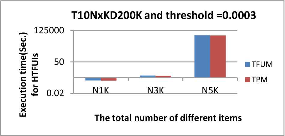
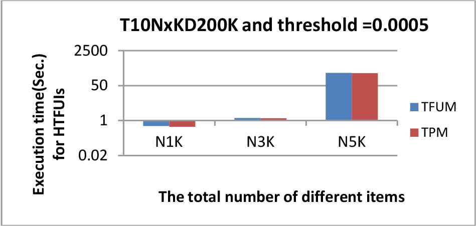
Experiments were first done for comparing the execution time and the numbers of upper-bound itemsets under a single minimum threshold and under multiple minimum thresholds. We compare various N values for the three T4NxKD200K datasets. Figures 3–5 show the execution time along with various λDIFF values for the three datasets. Here the symbol λDIFF represents the lower bound of the minimum thresholds of all the items in databases and can be regarded as the minimum threshold, λmin, in TFUM, which uses only a single minimum utility threshold.

The execution time from the T10NxKD200K dataset along with λDIFF = 0.0003.
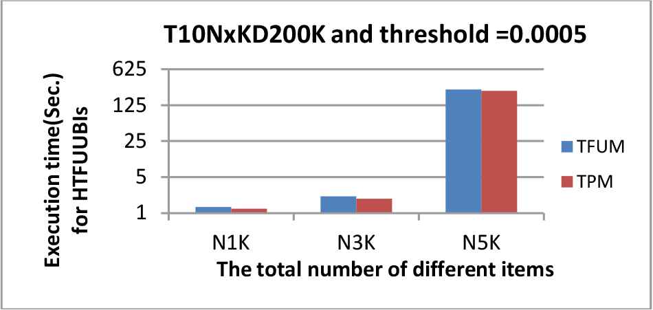
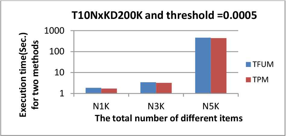
The execution time from the T10NxKD200K dataset along with λDIFF = 0.0005.
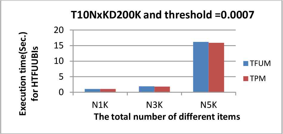
The execution time from the T10NxKD200K dataset along with λDIFF = 0.0007.
Note that in Figures 3 and 4, the y-axis use log-scale. Figures 6–8 show the numbers of upper-bound itemsets along with various λDIFF values for the three datasets. Similarly in Figures 6–8, the y-axis use log-scale.
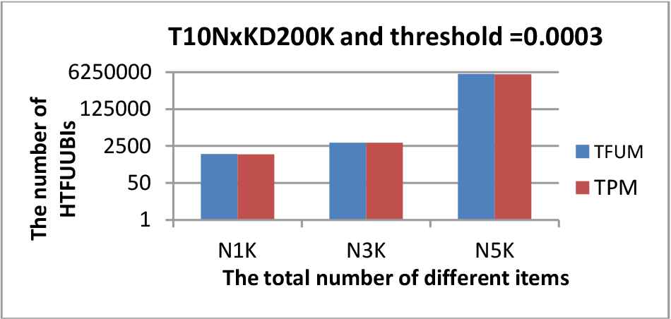
The numbers of upper-bound itemsets from the T10NxKD200K dataset along with λDIFF = 0.0003.
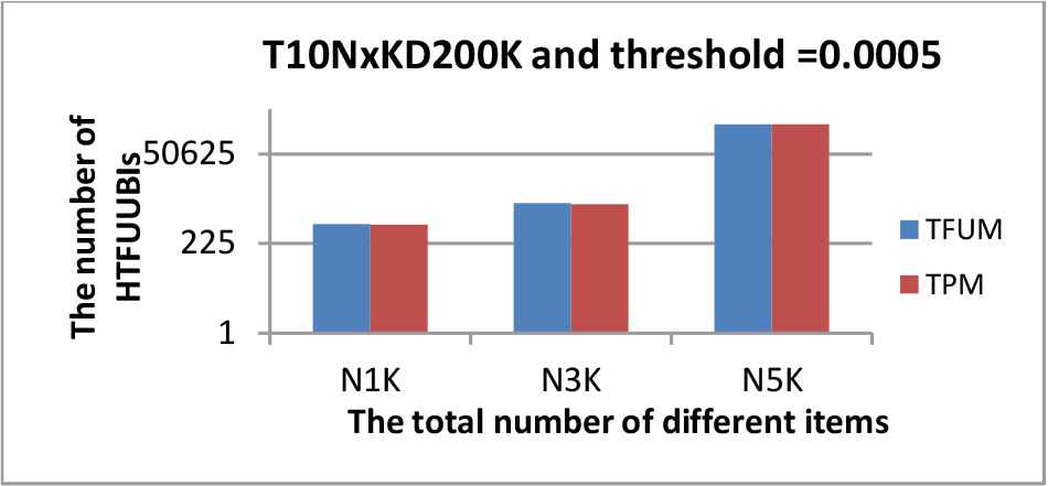
The numbers of upper-bound itemsets from the T10NxKD200K dataset along with λDIFF = 0.0005.
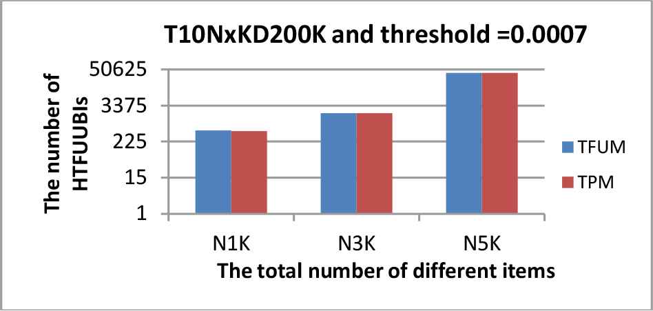
The numbers of upper-bound itemsets from the T10NxKD200K dataset along with λDIFF = 0.0007.
It could be observed from these figures that the execution time and the numbers of high upper-bound itemsets derived by our proposed TPM algorithm were less than those of TFUM using only a single minimum standard. The main reason for this is that all the items in the traditional TFUM were treated uniformly. That is, it did not consider the different property of items, and thus the minimum threshold was the same for all items in a database. Compared to the traditional TFUM, the new algorithm considers different minimum standards for items. In other words, in the experiments, since the minimum standards of all the items were not smaller than the user-specified lower-bound, which was used as the single minimum fuzzy utility threshold in the traditional TFUM, the number of high utility itemsets derived by our proposed TPM algorithm must be less than or equal to that by the TFUM method. In addition, as mentioned in Line 37 of Algorithm 3 and Line 61 of Algorithm 4, the integrated minimum threshold would gradually increase when a larger number of items were included in an itemset at later passes during the process of finding high upper-bound itemsets (HTFUUBI).
5.2. Evaluation of Execution Efficiency for Phase 2 in the Two Methods
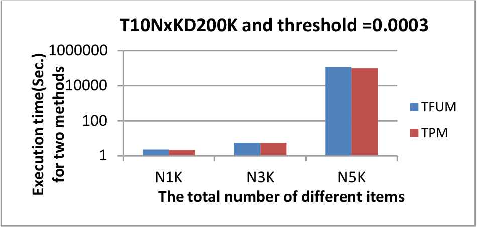
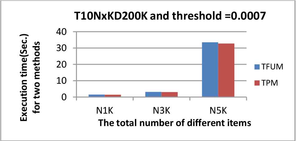
The same as before, the three synthetic datasets were conducted to assess the mining efficiency of the proposed TPM and the traditional TFUM for phase 2. Figures 9–11 show the execution efficiency of the two approaches (TPM and TFUM) for phase 2 under various λDIFF values. Figures 12–14 show the numbers of HTFUI itemsets of the two methods under various λDIFF values. Note that in Figures 9 and 10, the y-axis use log-scale.
Performance comparison of the two phase 2 approaches for T10NxKD200K dataset under λDIFF = 0.0003.
Performance comparison of the two phase 2 approaches for T10NxKD200K dataset under λDIFF = 0.0005.

Performance comparison of the two phase 2 approaches for T10NxKD200K dataset under λDIFF = 0.0007.
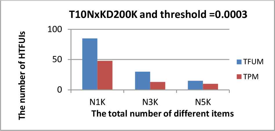
The numbers of high temporal fuzzy utility itemset (HTFUI) itemsets from the T10NxKD200K dataset along with λDIFF = 0.0003.
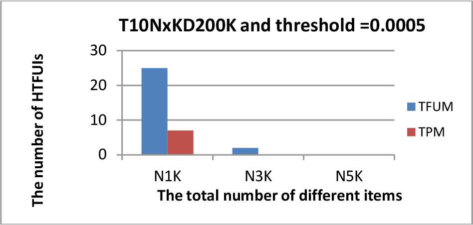
The numbers of high temporal fuzzy utility itemset (HTFUI) itemsets from the T10NxKD200K dataset along with λDIFF = 0.0005.
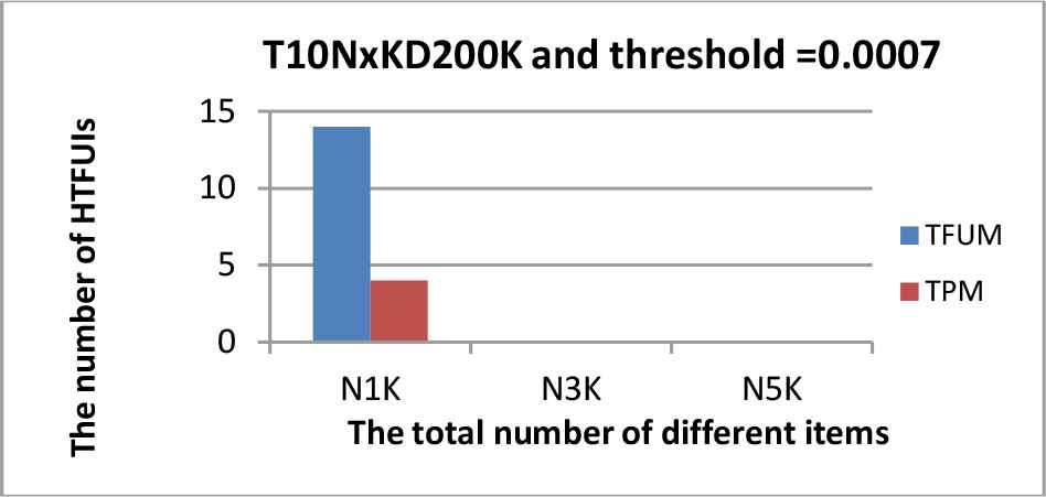
The numbers of high temporal fuzzy utility itemset (HTFUI) itemsets from the T10NxKD200K dataset along with λDIFF = 0.0007.
It could be observed from these figures that the execution time of phase 2 and the numbers of HTFUI itemsets derived by our proposed TPM algorithm was less than those of TFUM using only a single minimum standard. Again, this is because all the items in the traditional TFUM were treated uniformly when compared to the TPM algorithm. That is, TFUM did not consider the different properties of items, and thus the minimum threshold was the same for all items in a database. However, the TPM algorithm considers different minimum standards for items. Thus, the traditional temporal fuzzy utility mining algorithm mined more HTFUIs than the proposed one. Hence, the proposed framework using multiple minimum constraints might be a proper framework where items had different minimum constraints. Besides, both the algorithms would get more high upper-bound itemsets when the minimum threshold was smaller.
5.3. Evaluation of Execution Efficiency for the Two Methods
The three datasets were conducted to assess the total mining efficiency of the two phases for the proposed TPM and the traditional TFUM. Figures 15–17 show the execution efficiency of the two approaches (TPM and TFUM) for the databases under various λDIFF values.
Performance comparison of the two algorithms for T10NxKD200K dataset under λLB = 0.0003.
Performance comparison of the two algorithms for T10NxKD200K dataset under λLB = 0.0005.
Performance comparison of the two algorithms for T10NxKD200K dataset under λLB = 0.0007.
We could observe that the TPM approach was better than the traditional TFUM approach with a single threshold regarding execution efficiency when λDIFF increased. The main reason is that with the help of the minimum constraints, only the itemsets which satisfied their own minimum thresholds and not the lowest minimum threshold value for all items could be generated in the databases. Accordingly, the proposed TPM approach did not need to derive more itemsets than the traditional TFUM approach using only a single minimum threshold. Overall, the proposed TPM outperformed the traditional TFUM approach in execution efficiency under a variety of parameter settings.
The proposed TPM method can be thought of as a general algorithm for temporal fuzzy utility problem. When the multi-conditional thresholds for the proposed TPM method are identical for all items, TPM can be considered as the TFUM method. In this case, the TPM method with identical values may require a few more execution time than the TFUM method because the former needs to find itemset constraints.
6. CONCLUSION AND FUTURE WORK
This study proposes a new mining problem named temporal fuzzy utility mining with multi-conditional minimum thresholds, which goes further to consider the fuzzy viewpoint of applying the multiple minimum constraints of itemsets in a database when items have different standards. Different from the traditional temporal fuzzy utility mining with considering only a single minimum standard, the nature of items in our study can be reflected under different minimum thresholds. The experimental results also showed that our proposed TPM approach derived fewer itemsets than the TFUM approach and had good performance from both the effectiveness of multi-conditional viewpoint and the execution efficiency. Besides, the proposed TPM approach can be thought of as a generalized version of the previous TFUM approach and can execute the work that TFUM performs.
In the future, we will attempt to handle the maintenance problems of temporal fuzzy utility mining when new transactions are inserted, old transactions are modified even if overdue transactions are deleted.
REFERENCES
Cite this article
TY  - JOUR
AU  - Wei-Ming Huang
AU  - Tzung-Pei Hong
AU  - Ming-Chao Chiang
AU  - Jerry Chun-Wei Lin
PY  - 2019
DA  - 2019/05/11
TI  - Using Multi-Conditional Minimum Thresholds in Temporal Fuzzy Utility Mining
JO  - International Journal of Computational Intelligence Systems
SP  - 613
EP  - 626
VL  - 12
IS  - 2
SN  - 1875-6883
UR  - https://doi.org/10.2991/ijcis.d.190426.001
DO  - 10.2991/ijcis.d.190426.001
ID  - Huang2019
ER  -