
Time-Based Dance Scheduling for Artificial Bee Colony Algorithm and Its Variants
- DOI
- 10.2991/ijcis.d.190425.001How to use a DOI?
- Keywords
- ABC algorithm; Employed bees; Time-based dance scheduling
- Abstract
Artificial Bee Colony (ABC) algorithm inspired by the intelligent source search and consumption characteristics of the real honey bees is one of the most powerful optimization techniques. Although the existing behaviours of the honey bees in standard ABC algorithm are capable of producing optimal or near optimal solutions for the vast majority of the problems, there are still some intelligent characteristics that are not modeled yet such as decision-making mechanism used by employed bees to determine when the dancing will be completed. In this study, a mechanism that adjusts the dancing durations of the employed bees according to the fitness values of the associated food sources is proposed and integrated to the standard ABC algorithm and its well-known variants. Experimental studies on a set of complex continuous numerical problems showed that the newly proposed dance scheduling approach significantly improved the search and consumption characteristics of the artificial bees of the standard ABC algorithm and its some variants.
- Copyright
- © 2019 The Authors. Published by Atlantis Press SARL.
- Open Access
- This is an open access article distributed under the CC BY-NC 4.0 license (http://creativecommons.org/licenses/by-nc/4.0/).
1. INTRODUCTION
The intelligent characteristics such as division of labor, self-organization, multiple interactions of the some species especially living together as swarms or colonies in nature have lead to emerge a new research area called swarm intelligence. Researchers have tried to model the mentioned characteristics of the agents or individuals and proposed various swarm intelligence–based optimization techniques over the last two decades [1,2]. Among these swarm intelligence–based techniques, Artificial Bee Colony (ABC) algorithm gained a special position when the robust and flexible bee phases, good balance between exploitation and exploration operations, easily implementable and configurable steps, and finally requiring less control parameters were considered [3–5].
The studies that focus on improving the performance of the ABC algorithm can be classified into three major groups as illustrated in Figure 1. In the first group of these studies, the mathematical models used in bee phases of the ABC algorithm are changed with information provided by other solutions or modified with well-known techniques. Tsai et al. changed the candidate generation schema of the onlooker bees of the standard ABC algorithm by utilizing the Newtonian Law of universal gravitation and introduced the intersection ABC (IABC) algorithm [6]. In the proposed ABC algorithm, an analogy between food sources and masses is formed and a gravitational force calculated between two masses is used as a coefficient [6]. Zhu and Kwong also modified the candidate generation schema of the onlooker bees and proposed gbest-guided ABC (GABC) algorithm [7]. In GABC algorithm, a candidate solution was produced by utilizing the information of the best food source in addition to the information of a randomly determined neighbor [7]. Akay and Karaboga used a probabilistic selection schema in which the decision whether a parameter will be changed or not is made by comparing a random value with a new control parameter called MR [8]. Experimental studies with the proposed ABC algorithm on solving high-dimensional numeric and constrained engineering problems showed that perturbing more than one parameters can increase the solution qualities [8]. Gao et al. introduced two new ABC algorithm variants called ABC/best/1 and ABC/best/2. ABC/best/1 and ABC/best/2 algorithms are based on generating candidate solutions by the guidance of the best solution. Gao et al. also proposed a new ABC algorithm for which an employed or an onlooker bee produces new solutions by using two randomly selected neighbor solutions rather than utilizing only one randomly determined solution [9]. In other study, they combined advantageous sides of different search and multi-population techniques into together and introduced ILABC algorithm [10]. For ILABC algorithm, the whole colony is divided into subcolonies and employed bee phase of the ABC algorithm is powered by the best solution in the corresponding subcolony while onlooker bee phase of the ABC algorithm is directed with the global best solution of the whole colony [10].
Abro and Saleh changed the scout bee phase of the original ABC algorithm by proposing a new scouting characteristics that are based on receiving information of the best food source found so far rather than receiving information of a randomly determined one [11]. Tran et al. introduced a new ABC algorithm–based clustering technique called enhanced ABC algorithm/K-means for short EABCK [12]. In EABCK, the search equations used by employed and onlooker bee phases are changed with the additions of the arithmetic mutation operator and the information of the global best solution [12]. Hu et al. introduced a novel communication model abbreviated as HCM for ABC algorithm [13]. In the HCM model, the whole colony is divided into groups. The group of HCM contains one or more species that can be in communication with each other according to the island model [13]. Each group at one level up is related with a community. All of the species can set their information through groups to the communities [13]. He and Ma proposed a new ABC algorithm in which the numbers of the randomized Halton sequence is used [14]. A series of experiments with Halton sequence–based ABC algorithm demonstrated that Halton sequence–based initialization increases the convergence speed and accuracy of the solutions compared to the opposition-based, chaotic, and pure randomized initializations [14]. Luo et al. changed the probabilistic search mechanism of the standard ABC algorithm with a deterministic selection procedure in which the best food source is consumed by onlookers until the completion of the onlooker bee phase [15].
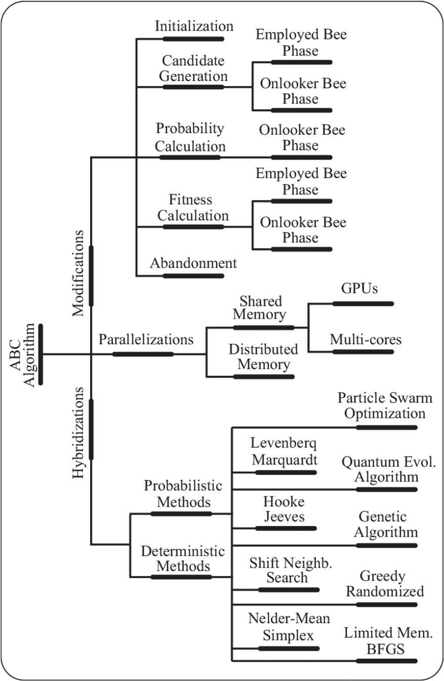
A chart for the studies about the Artificial Bee Colony (ABC) algorithm.
The second group of studies is devoted to the hybridization of the ABC algorithm with other intelligent methods. Baykasoglu et al. modified ABC algorithm with shift neighborhood search and greedy randomized adaptive search techniques and tested its performance on solving generalized assigned problem [16]. Kang et al. used ABC algorithm with Nelder–Mean Simplex method and proposed Hybrid Simplex ABC (HSABC) algorithm [17]. Kang et al. also integrated Hookee Jeeves pattern search approach to the ABC algorithm and introduced Hookee Jeeves ABC (HJABC) algorithm [18]. Ozturk and Karaboga combined ABC algorithm with Levenberg–Marquardt algorithm for training neural networks [19]. Duan et al. proposed a new hybrid-solving technique for continuous problems by utilizing ABC and Quantum Evolutionary algorithms [20]. Lavanya and Srinivasan hybridized ABC and genetic algorithm (GA) and tested mentioned hybrid optimization algorithm on solving training problem related with the neural networks [21]. Badem et al. combined ABC and limited memory-based BFGS algorithms and used their new variant for training deep neural networks [22]. Badem et al. also investigated the performance of their hybridized ABC algorithm on solving numerical benchmark problems [23].
Finally, the third group of the studies can be directly related with the parallelized implementations of the ABC algorithm. Narasimhan parallelized ABC algorithm by dividing the whole colony into equally sized subcolonies running simultaneously [24]. Banharnsakun et al. proposed a parallel ABC algorithm for distributed memory-based architectures [25]. Subotic et al. utilized the computation power of the multicore systems by running multiple colonies for ABC algorithm [26,27]. In the multiple colony-based parallelization, after completion of a predetermined number of cycles, the best food sources between colonies were exchanged [26,27]. Parpinelli et al. investigated parallelized ABC algorithm with different work schemas including master-slave, multi-hive with migration, and hybrid hierarchical [28]. Basturk and Akay analyzed coarse-grained model-based parallel ABC algorithm for solving numerical optimization problems and training neural networks [29]. Karaboga and Aslan proposed a new emigrant creation strategy for parallelized implementation of the ABC algorithm [30].
For the vast majority of the studies about ABC algorithm, it can be generalized that intelligent behaviours modeled in the standard ABC algorithm are found enough and improved versions of the ABC algorithm are based on integrating useful properties of the other techniques to the existing workflow of the algorithm. However, some intelligent characteristics of the employed foragers that are not modeled or tried to be managed by the randomized operations should be the first choice for further improving the performance of the ABC algorithm. In this study, one of the most important forager characteristics related with the determination of the fitness-based dancing durations is modeled and integrated to the standard ABC algorithm and its commonly used variants. Experimental studies on a set of benchmark problems showed that ABC algorithm and its variants for which the selection of the food sources being consumed is managed by probabilistic operations are significantly improved in terms of solution qualities and convergence speeds. The rest of the paper is organized as follows: In Section 2, fundamental steps of the ABC algorithm and its variants are introduced. Properties of the newly introduced fitness-based dancing mechanism is given in Section 3. Experimental studies with different control parameters and comparisons between algorithms are presented in Section 4. Finally, in Section 5, conclusion and future works are summarized.
2. STANDARD ABC ALGORITHM
In real honey bee colonies, the search operations for food sources are successfully managed by three group of bees called employed, onlooker, and scout bees and two different behaviour modes related to the consumption and abandonment of a source. Employed bees are responsible for finding food sources around the previously visited ones and carrying nectars to the hive [31–34]. When an employed bee turns back to the hive, she shares information about the utilized food source with the onlooker bees waiting on the dance area. The information shared by the employed bees with dances have an important effect on the source selection procedures of the onlookers. If a food source is rich in terms of nectar amount and worth at consuming by other foragers, the employed bee associated with this food source stays longer on the dance area and continues dancing for attracting more onlooker bees to the mentioned food source compared to other ones. Finally, the last group of bees, scout bees, searches food sources randomly without using information provided by employed bees and the total number of scouts is roughly
By considering the properties of the honey bees in foraging, Karaboga proposed a new swarm intelligence–based optimization technique called ABC algorithm. In ABC algorithm, the position of a food source corresponds to a possible solution of the problem being optimized and the nectar amount of the food source is directly related to the quality of the solution. With the discovery of the initial solutions or food sources by scout bees, ABC algorithm tries to improve these solutions with cyclic-iterative employed, onlooker and scout bee phases until satisfying the previously determined termination criteria [31–34].
2.1. Generating Initial Solutions
When solving a
In Equation (1),
2.2. Sending Employed and Onlooker Bees to Food Sources
The standard implementation of the ABC algorithm relates an employed bee with only one food source, in other words, the number of food sources is equal to the number of employed bees. As mentioned before employed bees are responsible for finding new food sources within the neighborhood of the memorized ones. After completion of source assignment, an employed bee determines a candidate food source in ABC algorithm by utilizing the Equation (2).
In Equation (2),
Assume that the fitness value of the
When all of the employed bees turn back to the hive, they share information about the memorized food sources with onlooker bees. For recruiting more onlookers to the qualified sources, ABC algorithm determines selection probabilities for each food source according to the Equation (4) given below. As seen from the Equation (4), the selection probability of the
Algorithm 1: Fundamental steps of the ABC algorithm
1: Initialization:
2: Generate SN initial food sources by using Equation (1).
3: Assign value to maximum fitness evaluations,
4: Set evaluation counter,
5: Repeat
6: //Employed bee phase
7: for
8: if
9: Generate
10: if
11: Change
12: end if
13:
14: end if
15: end for
16: //Onlooker bee phase
17:
18: Find probability values of each food source by using Equation (4).
19: while
20: if
21:
22: Generate
23: if
24: Change
25: end if
26:
27: end if
28:
29: end while
30: //Scout bee phase
31: if
32: Determine the abandoned food source using
33: Generate a new source for abandoned food source by using Equation (1).
34:
35: end if
36: Until
2.2.1. Abandoning food sources
In ABC algorithm, when the employed and onlooker bee phases are examined, it is clearly seen that both employed and onlooker bees consume existing food sources. However, if a food source is not worth consuming any more or it is exhausted completely, is should be changed with another food source. This type of mechanism in ABC algorithm is maintained by comparing trial counters with a specific control parameter called limit. In the scout bee phase, if there is a food source for which the trial counter exceeds the limit value at most, this food source is abandoned and the employed bee related with the abandoned food source becomes a scout for finding a new food source as described in Equation (1). Although ABC algorithm does not have a solid restriction about the values that can be assigned to the limit parameter, the colony size and number of parameters that are showed by
Initialization of the food sources and evaluating them with the employed, onlooker, and scout bee phases of the ABC algorithm can be analyzed more thoroughly from the Algorithm 1.
2.3. Different Candidate Generation Approaches in Variants of ABC Algorithm
The search equation used by employed and onlooker bee phases of the standard ABC algorithm is enough for different types of problems. However, some researches are also carried out for further improving convergence speed, qualities of the solutions, and solving capabilities of the algorithm. One of the most successful modifications in search equation of the standard ABC algorithm is made by Zhu and Kwong [7]. Zhu and Kwong proposed a new ABC algorithm called GABC algorithm. When the
Another important modification to the search equation of the standard ABC algorithm is presented by Gao et al. Gao et al. proposed two ABC variants called ABC/best/1 and ABC/best/2 by utilizing the search equations in Equations (7) and (8), respectively [9]. For both Equations (7) and (8),
The utilization approach from the best food source to direct the newly discovered solutions is handled by Luo et al. in a different manner [15]. When the candidate generation schema of the ABC algorithm is analyzed, it is clearly seen that the candidate solution is produced by modifying only one parameter and updating different dimensions of the problem still requires long evaluation times. By considering the mentioned effect of the single dimension-based update mechanism, Luo et al. decided to directly update best food source found so far with the selected food sources chosen by the onlookers as described in Equation (9) below for converge-onlookers ABC (COABC) algorithm [15].
The global best solution found so far or the best solution found in the current evaluation is the most appropriate information source for directing search equations. However, if the global best food source cannot be improved after completion of a long evaluation period, the algorithm can get stack of a local optimum or the convergence to the global optimum is delayed because of the oscillations between the best and neighbor food sources. To overcome these possible disadvantages stemmed from the known oscillation phenomenon, Gao et al. generate a candidate food source by using two randomly determined solution as in the Equation (10) [35]. In Equation (10),
In the vast majority of the studies, the coefficients used in the search equations are determined randomly between
When the search equations used by standard ABC algorithm and its mentioned variants are considered, it is clearly seen that one additional term is directly used without applying a multiplication, addition, or subtraction operation. In order to decrease the dependency of the changed parameter to the original value of it, Tran et al. modeled the arithmetic crossover method for the candidate generation procedure of the ABC algorithm as in the Equation (12) [12]. In Equation (12),
3. Time-Based Dance Scheduling for Employed Foragers
When the workflow of the employed, onlooker, and scout bee phases and used mathematical models for consuming, choosing, or abandoning sources are evaluated, it is clearly seen that there is a good balance between implementation flexibility of the ABC algorithm and intelligent behaviours of the real honey bees. Although ABC algorithm is capable of handing various optimization problems successfully with its default definitions because of the mentioned subtle balance, some important bee characteristics still need to be modeled and integrated to the standard the ABC algorithm.
One of the most important bee characteristics that are neither modeled by standard implementation of the ABC algorithm nor its variants is directly related with the dancing durations of the employed foragers. In the standard ABC algorithm, all of the employed bees start dancing with the completions of their source searching and they continue until all of the onlookers choose food sources. However, in a real honey bee colony, the existences of the employed foragers on the dance area are directly related with the qualities of the food sources being consumed. If a food source consumed by an employed bee is rich and the fitness value assigned to this food source is high compared to other food sources, the employed forager of the mentioned food source stay longer on the dance area for attracting more onlookers to this food source. While some of the employed foragers related with the qualified sources wait on the dance area and perform different dance figures, some of them related with the poor sources leave the dance area and fly without waiting onlooker bees. In Figure 2, how the number of employed bees is changing according to the time is illustrated for both artificial and real bees. The employed bees signed with red circles in Figure 2 associated with the qualified food sources. While the number of employed bees on the dance area decreases as time goes by in a real honey bee colony, standard ABC algorithm protects all of the employed bees on the dance area until the whole onlooker bees are sent.
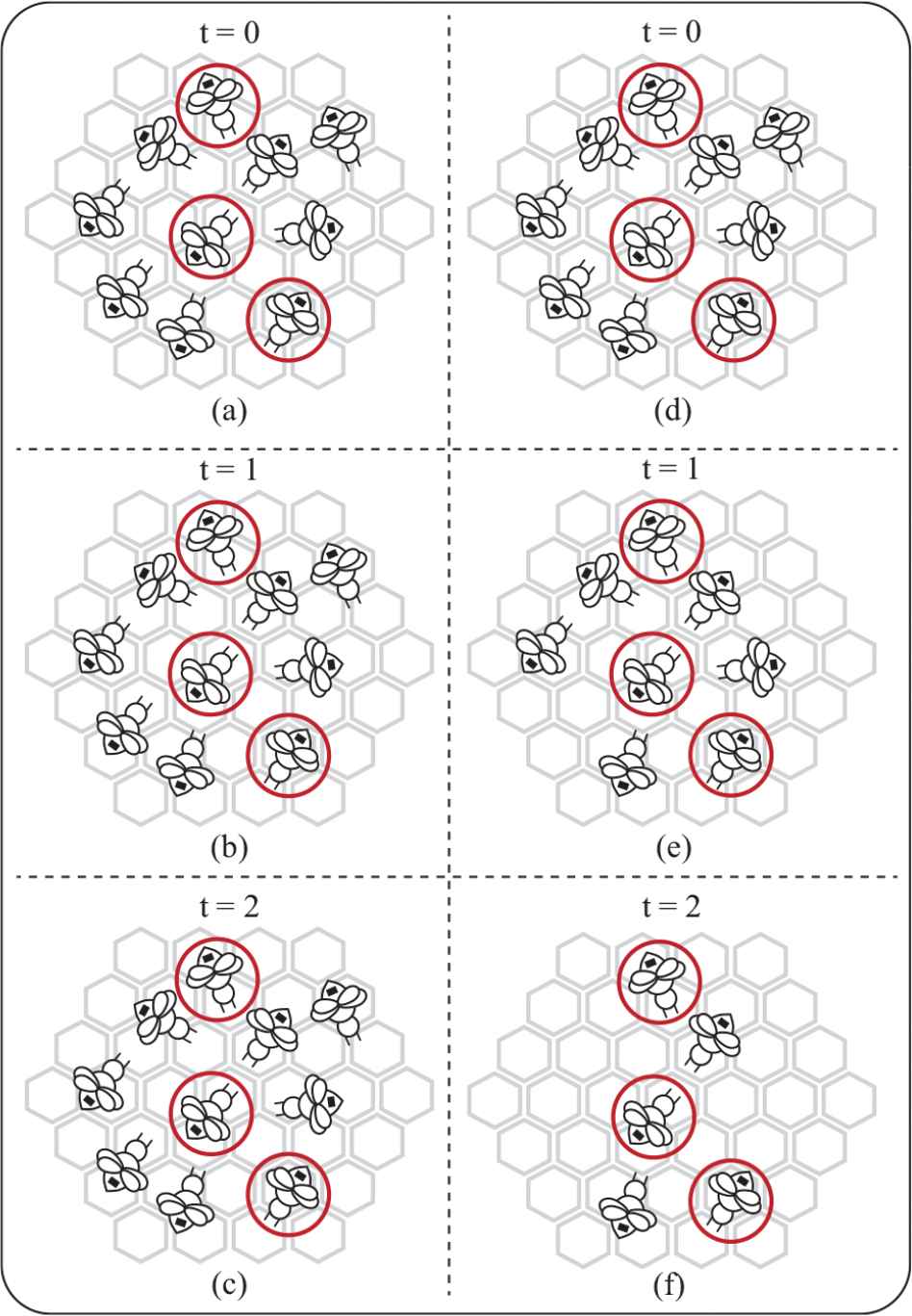
Employed bees on the dance area for Artificial Bee Colony (ABC) (a)–(c) and real honey bee (d)–(f) colonies.
At the first sense, mentioned characteristics related with the employed bees might be thought as a routine and not be considered as an intelligent behaviour. But, determining dancing durations proportional with the fitness values of the memorized solutions can help sending more onlookers to the qualified solutions. The main idea lying behind in this study is directly based on the modeling of the dancing start and finish decisions made by employed bees. In order to model the mentioned characteristics of the employed bees, a new control mechanism called time-based dance scheduling, for short ts, is introduced. With the ts model, dancing duration of an employed bee is determined by considering the fitness value of the memorized food source and decremented by also considering the fitness value of the same source for each selection attempt in on looker bee phase. If the dancing duration of an employed forager becomes equal to zero, this employed bee leaves the dance area while others with qualified sources are still on the dance area.
In ts mechanism, initial dancing durations of the employed bees are determined as their indexes in the vector of fitness values sorted in ascending order. Assume that there are SN food sources consumed by SN different employed bees and
As easily seen from the Equation (2) that is used to generate candidate solutions for standard ABC algorithm, one food source except than the selected one is required at least to satisfy the multiple interactions between solutions. In other words, there should be at least two different employed bees on the dance area. In ts mechanism, if the current time duration of an employed bee is equal to
Algorithm 2: Onlooker bee phase of ABC algorithm modified with ts mechanism
1: //Onlooker bee phase
2:
3: for
4:
5: end for
6:
7:
8: Find probability values of each food source by using Equation (4).
9:
10: while
11:
12: if
13:
14: Generate
15: if
16: Change
17: end if
18:
19: end if
20: if
21:
22: for
23: Update
24: end for
25:
26: if
27:
28: for
29:
30: end for
31: end if
32: end if
33:
34: end while
4. Experimental Studies
In order to analyze the effects of the ts mechanism on solving capabilities of the ABC, GABC, ABC/best/1, ABC/best/2, COABC, CABC, ERABC, and EABC algorithms,
| No | Function | Related Basic Functions | Reference |
|---|---|---|---|
| Rotated Bent Cigar function | Bent Cigar function | 100 | |
| Rotated Discus function | Discus function | 200 | |
| Shifted and Rotated Weierstrass function | Weierstrass function | 300 | |
| Shifted and Rotated Schwefel's function | Schwefel's function | 400 | |
| Shifted and Rotated Katsuura function | Katsuura function | 500 | |
| Shifted and Rotated HappyCat function | HappyCat function | 600 | |
| Shifted and Rotated HGBat function | HGBat function | 700 | |
| Shifted and Rotated Expanded Griewank's plus Rosenbrock's function | Griewank's function Rosenbrock's function | 800 | |
| Shifted and Rotated Expanded Scaffer's |
Expanded Scaffer's |
900 | |
| Hybrid function 1 (N = 3) | Schwefel's function Rastrigin's function High-conditioned elliptic | 1000 | |
| Hybrid function 2 (N = 4) | Griewank's function Weierstrass function Rosenbrock's function Scaffer's |
1100 | |
| Hybrid function 3 (N = 6) | Katsuura function HappyCat function Griewank's function Rosenbrock's function Schwefel's function Ackley's function | 1200 | |
| Compositional function 1 (N= 4) | Rosenbrock's function High-conditioned elliptic Bent Cigar function Discus function | 1300 | |
| Compositional function 2 (N = 3) | Schwefel's function Rastrigin's function High-conditioned elliptic | 1400 | |
| Compositional function 3 (N = 5) | HGBat function Rastrigin's function Schwefel's function Weiestrass function High-conditioned elliptic | 1500 |
Benchmark functions used in the experiments.
For all of the ABC algorithms, ABC, GABC, ABC/best/1, ABC/best/2, COABC, CABC, ERABC, EABC, and their ts mechanism based models named ts-ABC, ts-GABC, ts-ABC/best/1, ts-ABC/best/2, ts-COABC, ts-CABC, ts-ERABC, and ts-EABC algorithms, two different values including
When the results given in the Tables 2–9 are investigated, it is clearly seen that ts mechanism improves the qualities of the final solutions for some of the ABC algorithms including standard ABC, GABC, ABC/best/1, ABC/best/2, CABC, and EABC. All of these algorithms select a food source or sources randomly for generating candidates around it as is done by real honey bees and also require selection of food source or sources to satisfy the multiple interaction between solutions. The main idea lying behind the ts mechanism is that the dancing durations of the employed bees should be adjusted according to the fitness values of the memorized food sources and the employed bees with more qualified food sources should be kept on the dance area as time goes by. With ts mechanism, the existence of an employed bee on dance area is proportional with its fitness value and choosability of a qualified food source by an onlooker is increased.
Although this mentioned realistic approach is suitable with the candidate generation schema of the standard ABC, GABC, ABC/best/1, ABC/best/2, CABC, and EABC algorithms, candidate generation schemas of the COABC and ERABC algorithms restrict the improving effect of the ts mechanism. In COABC algorithm, the fitness-based probabilistic selection characteristics of the onlookers are changed with a deterministic selection schema and all of the onlooker bees are sent to the global best food source for increasing the early convergence performance of the algorithm compared to its standard implementation. In other words, onlooker bees have no chance of selecting food sources for consuming and ts mechanism does not show its improving effect on the performance of the onlooker bees. For the ERABC algorithm, the fitness value of the food source used as a coefficient in the candidate production deteriorates the effect of the additional term if the fitness value is relatively close to zero. When the difficulties of the problems and small number of fitness evaluations are taken into account, multiplying the second term of the equation used for generating a candidate solution with the fitness value of the food source limits the contribution of the selected sources of the ts mechanism.
In order to analyze that how the ts mechanism contributes to the convergence performance of the ABC algorithm and its variants, the curves given in the Figure 3 below can be controlled. The convergence curves in Figure 3 are generated for ABC algorithms with
| Function | ABC | ts-ABC | GABC | ts-GABC | ABC/best/1 | ts-ABC/best/1 | ABC/best/2 | ts-ABC/best/2 | |
|---|---|---|---|---|---|---|---|---|---|
| Mean | 2.716658e+09 | 7.715196e+08 | 8.210307e+08 | 6.252916e+08 | 4.776608e+08 | 1.207570e+09 | 7.607792e+08 | 3.565431e+08 | |
| Std.Dev. | 2.619777e+09 | 1.318637e+09 | 6.477353e+08 | 5.853795e+08 | 3.162419e+08 | 8.886205e+08 | 3.439542e+08 | 3.568213e+08 | |
| Mean | 3.870378e+04 | 3.900769e+04 | 4.790570e+04 | 3.855270e+04 | 4.100352e+04 | 3.692275e+04 | 4.605250e+04 | 4.583296e+04 | |
| Std.Dev. | 1.313293e+04 | 1.407367e+04 | 1.806861e+04 | 1.567433e+04 | 1.429170e+04 | 9.994693e+03 | 2.342800e+04 | 1.460064e+04 | |
| Mean | 3.114588e+02 | 3.103083e+02 | 3.103419e+02 | 3.099561e+02 | 3.100924e+02 | 3.099762e+02 | 3.105299e+02 | 3.100281e+02 | |
| Std.Dev. | 1.357763e+00 | 1.280487e+00 | 1.038200e+00 | 1.232346e+00 | 1.287297e+00 | 1.577455e+00 | 9.663669e-01 | 1.162901e+00 | |
| Mean | 1.521087e+03 | 1.062533e+03 | 1.439194e+03 | 9.610165e+02 | 1.433784e+03 | 1.102033e+03 | 1.545442e+03 | 1.031898e+03 | |
| Std.Dev. | 2.335970e+02 | 2.680053e+02 | 2.979608e+02 | 2.266523e+02 | 2.346407e+02 | 2.695440e+02 | 2.282057e+02 | 1.590212e+02 | |
| Mean | 5.023907e+02 | 5.020619e+02 | 5.026821e+02 | 5.024273e+02 | 5.027842e+02 | 5.029346e+02 | 5.027086e+02 | 5.025562e+02 | |
| Std.Dev. | 5.832669e-01 | 4.888150e-01 | 5.806247e-01 | 5.524283e-01 | 5.945906e-01 | 7.315304e-01 | 5.061681e-01 | 6.219925e-01 | |
| Mean | 6.037940e+02 | 6.024325e+02 | 6.024441e+02 | 6.011801e+02 | 6.016304e+02 | 6.020585e+02 | 6.019961e+02 | 6.012319e+02 | |
| Std.Dev. | 9.912625e-01 | 9.683091e-01 | 7.219408e-01 | 3.097634e-01 | 5.553237e-01 | 9.076719e-01 | 6.358408e-01 | 3.686968e-01 | |
| Mean | 7.293699e+02 | 7.148945e+02 | 7.159116e+02 | 7.088647e+02 | 7.088151e+02 | 7.151470e+02 | 7.121670e+02 | 7.072477e+02 | |
| Std.Dev. | 1.818570e+01 | 8.723010e+00 | 9.064312e+00 | 5.353068e+00 | 5.753663e+00 | 9.626231e+00 | 5.186575e+00 | 5.170760e+00 | |
| Mean | 1.527860e+03 | 8.457670e+02 | 9.631715e+02 | 9.074125e+02 | 8.555846e+02 | 1.620868e+03 | 9.139047e+02 | 8.279735e+02 | |
| Std.Dev. | 1.120934e+03 | 5.161738e+01 | 2.787490e+02 | 1.906604e+02 | 5.269011e+01 | 1.702608e+03 | 1.927086e+02 | 4.906995e+01 | |
| Mean | 9.042098e+02 | 9.040828e+02 | 9.041019e+02 | 9.040767e+02 | 9.040568e+02 | 9.041801e+02 | 9.041138e+02 | 9.040719e+02 | |
| Std.Dev. | 1.603778e-01 | 1.824507e-01 | 1.788973e-01 | 2.665699e-01 | 1.820721e-01 | 1.755280e-01 | 1.301141e-01 | 2.313002e-01 | |
| Mean | 1.178271e+06 | 1.003313e+06 | 6.124471e+05 | 5.362535e+05 | 3.990019e+05 | 7.659800e+05 | 3.458791e+05 | 5.988060e+05 | |
| Std.Dev. | 2.817892e+06 | 2.684644e+06 | 4.638055e+05 | 4.807917e+05 | 5.088393e+05 | 9.471498e+05 | 2.519023e+05 | 7.526227e+05 | |
| Mean | 1.114830e+03 | 1.111651e+03 | 1.112123e+03 | 1.109447e+03 | 1.113348e+03 | 1.113243e+03 | 1.110513e+03 | 1.110851e+03 | |
| Std.Dev. | 5.740322e+00 | 5.151412e+00 | 5.319018e+00 | 2.710290e+00 | 3.423248e+00 | 6.558813e+00 | 2.621291e+00 | 4.439402e+00 | |
| Mean | 1.510483e+03 | 1.444484e+03 | 1.496250e+03 | 1.434543e+03 | 1.475182e+03 | 1.453063e+03 | 1.501027e+03 | 1.443331e+03 | |
| Std.Dev. | 1.213293e+02 | 9.774738e+01 | 7.500678e+01 | 1.003511e+02 | 8.097253e+01 | 8.700342e+01 | 1.073091e+02 | 9.680262e+01 | |
| Mean | 1.702227e+03 | 1.664968e+03 | 1.666147e+03 | 1.650612e+03 | 1.652384e+03 | 1.699363e+03 | 1.663966e+03 | 1.650791e+03 | |
| Std.Dev. | 5.955833e+01 | 3.205841e+01 | 2.929865e+01 | 1.609759e+01 | 1.813559e+01 | 5.506221e+01 | 2.384845e+01 | 1.984467e+01 | |
| Mean | 1.621208e+03 | 1.613885e+03 | 1.615869e+03 | 1.613554e+03 | 1.614540e+03 | 1.615772e+03 | 1.616070e+03 | 1.614553e+03 | |
| Std.Dev. | 9.655584e+00 | 6.287893e+00 | 5.387226e+00 | 5.484613e+00 | 5.274835e+00 | 6.809948e+00 | 6.126974e+00 | 4.859516e+00 | |
| Mean | 1.919081e+03 | 1.963648e+03 | 1.964664e+03 | 1.964024e+03 | 1.931967e+03 | 1.925884e+03 | 1.952774e+03 | 1.933972e+03 | |
| Std.Dev. | 1.023101e+02 | 7.321057e+01 | 8.481114e+01 | 1.143008e+02 | 6.756013e+01 | 9.020307e+01 | 5.775669e+01 | 1.405099e+02 | |
ABC, Artificial Bee Colony; GABC, gbest-guided ABC; Std.Dev., standard deviation.
Comparison of ABC, GABC, ABC/best/1, ABC/best/2 algorithms, and their ts model–based variants with 30 bees on solving 10 dimensional problems.
| Function | COABC | ts-COABC | CABC | ts-CABC | ERABC | ts-ERABC | EABC | ts-EABC | |
|---|---|---|---|---|---|---|---|---|---|
| Mean | 1.154472e+08 | 1.276849e+09 | 6.557027e+08 | 2.228156e+08 | 2.062686e+10 | 2.170513e+10 | 1.403711e+09 | 1.125660e+09 | |
| Std.Dev. | 1.212249e+08 | 1.662275e+09 | 4.389131e+08 | 1.610762e+08 | 7.444188e+09 | 5.705464e+09 | 9.416702e+08 | 6.692855e+08 | |
| Mean | 4.012159e+04 | 5.020721e+04 | 4.756039e+04 | 4.329411e+04 | 8.033285e+07 | 7.006532e+07 | 3.715573e+04 | 4.231731e+04 | |
| Std.Dev. | 1.661216e+04 | 2.891368e+04 | 1.897498e+04 | 2.404596e+04 | 1.556228e+08 | 1.004056e+08 | 1.227938e+04 | 1.613730e+04 | |
| Mean | 3.097314e+02 | 3.095482e+02 | 3.107713e+02 | 3.100124e+02 | 3.149511e+02 | 3.157276e+02 | 3.109229e+02 | 3.100109e+02 | |
| Std.Dev. | 1.632631e+00 | 1.959432e+00 | 1.010609e+00 | 1.134983e+00 | 1.605396e+00 | 1.564906e+00 | 1.186810e+00 | 1.102924e+00 | |
| Mean | 8.104725e+02 | 8.284283e+02 | 1.245628e+03 | 8.068427e+02 | 3.246849e+03 | 3.294964e+03 | 1.542388e+03 | 1.122538e+03 | |
| Std.Dev. | 1.611879e+02 | 1.570734e+02 | 1.818175e+02 | 2.028760e+02 | 3.020462e+02 | 3.900027e+02 | 2.195640e+02 | 2.209403e+02 | |
| Mean | 5.018665e+02 | 5.021253e+02 | 5.025557e+02 | 5.026895e+02 | 5.055547e+02 | 5.053779e+02 | 5.025863e+02 | 5.025689e+02 | |
| Std.Dev. | 5.199851e-01 | 5.943225e-01 | 5.337103e-01 | 6.756078e-01 | 1.427629e+00 | 1.329793e+00 | 5.788205e-01 | 7.541843e-01 | |
| Mean | 6.007468e+02 | 6.008256e+02 | 6.018007e+02 | 6.011450e+02 | 6.089245e+02 | 6.095337e+02 | 6.024926e+02 | 6.020531e+02 | |
| Std.Dev. | 1.856181e-01 | 2.926697e-01 | 5.070661e-01 | 5.380740e-01 | 1.527262e+00 | 1.669186e+00 | 5.772861e-01 | 5.949175e-01 | |
| Mean | 7.008683e+02 | 7.028242e+02 | 7.123414e+02 | 7.043181e+02 | 8.284115e+02 | 8.248690e+02 | 7.162609e+02 | 7.114402e+02 | |
| Std.Dev. | 4.393814e-01 | 4.878875e+00 | 5.541202e+00 | 2.546816e+00 | 4.130395e+01 | 3.897871e+01 | 7.975968e+00 | 3.844121e+00 | |
| Mean | 8.182980e+02 | 3.361056e+04 | 9.950345e+02 | 8.267994e+02 | 1.055673e+06 | 1.564280e+06 | 1.543894e+03 | 9.113788e+02 | |
| Std.Dev. | 1.771768e+01 | 6.950828e+04 | 3.825697e+02 | 5.489403e+01 | 1.131215e+06 | 1.581205e+06 | 2.295640e+03 | 1.705232e+02 | |
| Mean | 9.039660e+02 | 9.039186e+02 | 9.041741e+02 | 9.040658e+02 | 9.046754e+02 | 9.045633e+02 | 9.041481e+02 | 9.040730e+02 | |
| Std.Dev. | 2.430996e-01 | 2.720800e-01 | 1.494516e-01 | 2.145972e-01 | 1.554074e-01 | 2.285790e-01 | 1.710996e-01 | 2.080785e-01 | |
| Mean | 5.175479e+05 | 1.656484e+06 | 9.674845e+05 | 5.750111e+05 | 8.814672e+07 | 5.983723e+07 | 4.107140e+05 | 4.635940e+05 | |
| Std.Dev. | 8.156218e+05 | 1.919514e+06 | 8.747779e+05 | 6.273505e+05 | 1.081411e+08 | 5.477027e+07 | 3.411544e+05 | 4.165436e+05 | |
| Mean | 1.110225e+03 | 1.112355e+03 | 1.112797e+03 | 1.112840e+03 | 1.255240e+03 | 1.291331e+03 | 1.114068e+03 | 1.114381e+03 | |
| Std.Dev. | 2.777537e+00 | 5.544708e+00 | 3.487721e+00 | 3.620990e+00 | 6.653285e+01 | 1.526035e+02 | 4.790630e+00 | 5.114736e+00 | |
| Mean | 1.509919e+03 | 1.456713e+03 | 1.502446e+03 | 1.470657e+03 | 2.720915e+03 | 5.470793e+03 | 1.475801e+03 | 1.460404e+03 | |
| Std.Dev. | 9.668761e+01 | 1.345258e+02 | 1.000146e+02 | 8.753230e+01 | 2.427922e+03 | 1.078440e+04 | 1.006706e+02 | 9.119755e+01 | |
| Mean | 1.660884e+03 | 1.666798e+03 | 1.675543e+03 | 1.649346e+03 | 3.057997e+03 | 2.707758e+03 | 1.683561e+03 | 1.681644e+03 | |
| Std.Dev. | 2.524741e+01 | 4.395416e+01 | 3.379650e+01 | 1.346389e+01 | 7.418433e+02 | 6.490447e+02 | 3.064096e+01 | 4.294427e+01 | |
| Mean | 1.611896e+03 | 1.612063e+03 | 1.616420e+03 | 1.613649e+03 | 1.697243e+03 | 1.699400e+03 | 1.616794e+03 | 1.616111e+03 | |
| Std.Dev. | 9.319448e+00 | 8.504274e+00 | 6.171834e+00 | 7.805774e+00 | 5.130750e+01 | 3.405484e+01 | 5.618579e+00 | 6.736457e+00 | |
| Mean | 1.912819e+03 | 1.981372e+03 | 1.992193e+03 | 1.944291e+03 | 2.251244e+03 | 2.247013e+03 | 1.970404e+03 | 1.898319e+03 | |
| Std.Dev. | 1.480665e+02 | 1.082278e+02 | 4.979468e+01 | 6.677492e+01 | 1.077732e+02 | 1.023842e+02 | 6.179183e+01 | 9.863263e+01 | |
ABC, Artificial Bee Colony; Std.Dev., standard deviation; COABC, converge-onlookers ABC.
Comparison of COABC, CABC, ERABC, EABC algorithms, and their ts model–based variants with 30 bees on solving 10 dimensional problems.
| Function | ABC | ts-ABC | GABC | ts-GABC | ABC/best/1 | ts-ABC/best/1 | ABC/best/2 | ts-ABC/best/2 | |
|---|---|---|---|---|---|---|---|---|---|
| Mean | 2.874022e+10 | 7.380010e+09 | 1.007479e+10 | 5.276032e+09 | 6.758463e+09 | 1.172245e+10 | 6.436318e+09 | 1.570801e+09 | |
| Std.Dev. | 1.297193e+10 | 5.655872e+09 | 3.406875e+09 | 2.379473e+09 | 2.022907e+09 | 6.545935e+09 | 1.956905e+09 | 6.339895e+08 | |
| Mean | 1.086945e+05 | 1.119868e+05 | 1.221693e+05 | 1.188624e+05 | 1.100295e+05 | 1.153404e+05 | 1.132975e+05 | 1.130321e+05 | |
| Std.Dev. | 1.484122e+04 | 1.982311e+04 | 2.172899e+04 | 1.680534e+04 | 1.335718e+04 | 1.660430e+04 | 1.911921e+04 | 1.763017e+04 | |
| Mean | 3.409215e+02 | 3.397359e+02 | 3.378629e+02 | 3.374135e+02 | 3.386195e+02 | 3.369604e+02 | 3.374306e+02 | 3.377273e+02 | |
| Std.Dev. | 1.649650e+00 | 2.755678e+00 | 2.630754e+00 | 2.135595e+00 | 1.797164e+00 | 2.358775e+00 | 2.575609e+00 | 2.825846e+00 | |
| Mean | 4.898264e+03 | 2.580050e+03 | 5.064316e+03 | 2.894777e+03 | 4.500458e+03 | 2.876139e+03 | 4.889962e+03 | 3.313030e+03 | |
| Std.Dev. | 6.113384e+02 | 5.291545e+02 | 4.783905e+02 | 3.890094e+02 | 4.181204e+02 | 3.933831e+02 | 3.874354e+02 | 6.045009e+02 | |
| Mean | 5.031803e+02 | 5.027337e+02 | 5.033885e+02 | 5.033083e+02 | 5.035661e+02 | 5.035613e+02 | 5.037563e+02 | 5.032828e+02 | |
| Std.Dev. | 4.187038e-01 | 4.000041e-01 | 5.478987e-01 | 6.720153e-01 | 5.577199e-01 | 8.071338e-01 | 6.932659e-01 | 7.988223e-01 | |
| Mean | 6.048440e+02 | 6.031434e+02 | 6.023862e+02 | 6.008796e+02 | 6.014326e+02 | 6.021869e+02 | 6.014521e+02 | 6.009001e+02 | |
| Std.Dev. | 5.489252e-01 | 8.100654e-01 | 4.980876e-01 | 3.014158e-01 | 5.737325e-01 | 9.341314e-01 | 5.414082e-01 | 2.784951e-01 | |
| Mean | 7.991826e+02 | 7.275427e+02 | 7.298575e+02 | 7.102252e+02 | 7.173405e+02 | 7.250216e+02 | 7.225398e+02 | 7.102095e+02 | |
| Std.Dev. | 2.650585e+01 | 1.656431e+01 | 8.298526e+00 | 5.696513e+00 | 6.798589e+00 | 1.420327e+01 | 6.665316e+00 | 5.334576e+00 | |
| Mean | 4.287487e+05 | 1.378647e+05 | 4.368237e+05 | 5.983792e+04 | 2.035833e+05 | 6.545443e+05 | 2.925450e+05 | 9.330454e+04 | |
| Std.Dev. | 7.306972e+05 | 3.014948e+05 | 4.998589e+05 | 1.291739e+05 | 2.376706e+05 | 8.537197e+05 | 3.429529e+05 | 1.902556e+05 | |
| Mean | 9.138568e+02 | 9.137548e+02 | 9.137144e+02 | 9.137025e+02 | 9.137695e+02 | 9.137312e+02 | 9.137964e+02 | 9.136917e+02 | |
| Std.Dev. | 1.394280e-01 | 2.223189e-01 | 2.428242e-01 | 2.539421e-01 | 2.351620e-01 | 1.824119e-01 | 1.912461e-01 | 2.466965e-01 | |
| Mean | 2.127051e+07 | 2.022547e+07 | 1.848871e+07 | 1.583745e+07 | 2.234886e+07 | 2.067039e+07 | 1.987510e+07 | 1.298141e+07 | |
| Std.Dev. | 1.253340e+07 | 1.477105e+07 | 1.245245e+07 | 8.948488e+06 | 1.368461e+07 | 1.135056e+07 | 1.141494e+07 | 9.495358e+06 | |
| Mean | 1.276733e+03 | 1.184721e+03 | 1.244496e+03 | 1.195046e+03 | 1.235538e+03 | 1.220965e+03 | 1.222708e+03 | 1.205167e+03 | |
| Std.Dev. | 4.835406e+01 | 6.138788e+01 | 6.823799e+01 | 4.665858e+01 | 4.697590e+01 | 4.593123e+01 | 3.709698e+01 | 4.323351e+01 | |
| Mean | 2.375565e+03 | 2.247250e+03 | 2.324325e+03 | 2.172248e+03 | 2.213273e+03 | 2.306675e+03 | 2.302794e+03 | 2.247399e+03 | |
| Std.Dev. | 2.687816e+02 | 2.582901e+02 | 2.949635e+02 | 2.971143e+02 | 2.226441e+02 | 3.301708e+02 | 1.775432e+02 | 1.907788e+02 | |
| Mean | 2.104460e+03 | 1.828667e+03 | 1.948367e+03 | 1.792256e+03 | 1.883473e+03 | 2.044204e+03 | 1.934404e+03 | 1.790321e+03 | |
| Std.Dev. | 2.372981e+02 | 5.794128e+01 | 1.098594e+02 | 6.554537e+01 | 9.786156e+01 | 2.085624e+02 | 1.313962e+02 | 5.703170e+01 | |
| Mean | 1.751087e+03 | 1.702420e+03 | 1.711827e+03 | 1.700929e+03 | 1.709403e+03 | 1.702241e+03 | 1.707517e+03 | 1.699666e+03 | |
| Std.Dev. | 5.320667e+01 | 2.527095e+01 | 3.303930e+01 | 3.102879e+01 | 2.464513e+01 | 2.616494e+01 | 2.327794e+01 | 2.261910e+01 | |
| Mean | 2.834826e+03 | 2.744596e+03 | 2.771290e+03 | 2.728688e+03 | 2.780323e+03 | 2.774281e+03 | 2.780808e+03 | 2.760362e+03 | |
| Std.Dev. | 1.673755e+02 | 1.888101e+02 | 1.025995e+02 | 1.404296e+02 | 1.541621e+02 | 7.125748e+01 | 6.876194e+01 | 7.925066e+01 | |
ABC, Artificial Bee Colony; GABC, gbest-guided ABC; Std.Dev., standard deviation.
Comparison of ABC, GABC, ABC/best/1, ABC/best/2 algorithms, and their ts model–based variants with 50 bees on solving 10 dimensional problems.
| Function | COABC | ts-COABC | CABC | ts-CABC | ERABC | ts-ERABC | EABC | ts-EABC | |
|---|---|---|---|---|---|---|---|---|---|
| Mean | 3.164912e+08 | 2.432697e+09 | 4.213069e+09 | 1.662524e+09 | 1.126799e+11 | 1.203574e+11 | 1.381121e+10 | 7.677647e+09 | |
| Std.Dev. | 2.656562e+08 | 2.901365e+09 | 1.362111e+09 | 1.980279e+09 | 1.674295e+10 | 1.604682e+10 | 4.524733e+09 | 2.034167e+09 | |
| Mean | 1.109747e+05 | 1.114874e+05 | 1.156213e+05 | 1.092496e+05 | 2.593265e+07 | 6.367834e+07 | 1.066621e+05 | 1.065415e+05 | |
| Std.Dev. | 1.736156e+04 | 2.328571e+04 | 1.368680e+04 | 1.934016e+04 | 4.388028e+07 | 1.152567e+08 | 1.514714e+04 | 1.476639e+04 | |
| Mean | 3.382132e+02 | 3.388512e+02 | 3.387512e+02 | 3.368393e+02 | 3.514851e+02 | 3.504493e+02 | 3.394028e+02 | 3.376025e+02 | |
| Std.Dev. | 3.233474e+00 | 3.235970e+00 | 2.260633e+00 | 2.321731e+00 | 2.252532e+00 | 1.907562e+00 | 1.608742e+00 | 2.334614e+00 | |
| Mean | 1.523955e+03 | 1.892381e+03 | 4.062849e+03 | 1.984803e+03 | 1.044373e+04 | 1.026075e+04 | 4.559737e+03 | 2.897692e+03 | |
| Std.Dev. | 2.959567e+02 | 3.508363e+02 | 4.860837e+02 | 3.525632e+02 | 5.556362e+02 | 6.761046e+02 | 4.054989e+02 | 3.774576e+02 | |
| Mean | 5.024467e+02 | 5.025580e+02 | 5.037371e+02 | 5.038306e+02 | 5.077238e+02 | 5.068617e+02 | 5.037361e+02 | 5.035170e+02 | |
| Std.Dev. | 6.704678e-01 | 7.032852e-01 | 5.744850e-01 | 5.592104e-01 | 1.125381e+00 | 1.324530e+00 | 6.015442e-01 | 6.824195e-01 | |
| Mean | 6.006283e+02 | 6.006307e+02 | 6.010139e+02 | 6.006387e+02 | 6.090965e+02 | 6.088120e+02 | 6.031234e+02 | 6.020081e+02 | |
| Std.Dev. | 1.273650e-01 | 1.488749e-01 | 3.611400e-01 | 1.282884e-01 | 6.612400e-01 | 6.706021e-01 | 5.126429e-01 | 6.451348e-01 | |
| Mean | 7.006613e+02 | 7.006936e+02 | 7.112184e+02 | 7.027842e+02 | 9.580329e+02 | 9.653756e+02 | 7.319813e+02 | 7.198583e+02 | |
| Std.Dev. | 5.442124e-01 | 8.342133e-01 | 4.705639e+00 | 1.780604e+00 | 4.258692e+01 | 5.020076e+01 | 9.941893e+00 | 4.318610e+00 | |
| Mean | 7.243095e+03 | 2.669283e+06 | 4.774664e+05 | 2.835704e+04 | 3.300064e+08 | 4.276526e+08 | 1.765466e+05 | 1.108185e+05 | |
| Std.Dev. | 1.309429e+04 | 5.625904e+06 | 1.174563e+06 | 2.994867e+04 | 1.552979e+08 | 2.739110e+08 | 2.465664e+05 | 2.229498e+05 | |
| Mean | 9.137645e+02 | 9.136050e+02 | 9.138267e+02 | 9.137794e+02 | 9.145035e+02 | 9.145490e+02 | 9.137334e+02 | 9.137312e+02 | |
| Std.Dev. | 2.382136e-01 | 3.080091e-01 | 1.970009e-01 | 2.153151e-01 | 1.896895e-01 | 1.687801e-01 | 2.212720e-01 | 1.845016e-01 | |
| Mean | 2.094852e+07 | 2.725651e+07 | 2.063197e+07 | 2.044892e+07 | 6.878707e+08 | 6.469510e+08 | 2.193600e+07 | 1.855870e+07 | |
| Std.Dev. | 1.998104e+07 | 2.108055e+07 | 1.038327e+07 | 1.094937e+07 | 4.492558e+08 | 4.894871e+08 | 1.192082e+07 | 1.233614e+07 | |
| Mean | 1.166063e+03 | 1.175308e+03 | 1.238166e+03 | 1.213256e+03 | 2.762385e+03 | 2.429241e+03 | 1.228487e+03 | 1.192017e+03 | |
| Std.Dev. | 5.333776e+01 | 6.377053e+01 | 4.197417e+01 | 5.559392e+01 | 6.295319e+02 | 3.544412e+02 | 4.505229e+01 | 3.053538e+01 | |
| Mean | 2.228561e+03 | 3.645217e+03 | 2.246239e+03 | 2.238476e+03 | 3.597975e+06 | 3.091981e+06 | 2.355412e+03 | 2.146743e+03 | |
| Std.Dev. | 3.091278e+02 | 3.562596e+03 | 1.829921e+02 | 2.076445e+02 | 5.189896e+06 | 5.901716e+06 | 2.392137e+02 | 2.623970e+02 | |
| Mean | 1.720122e+03 | 1.809039e+03 | 1.903756e+03 | 1.779245e+03 | 4.922260e+03 | 4.740386e+03 | 2.012509e+03 | 1.921969e+03 | |
| Std.Dev. | 4.716193e+01 | 9.806224e+01 | 1.280937e+02 | 6.685828e+01 | 1.031560e+03 | 1.150095e+03 | 1.151269e+02 | 8.730109e+01 | |
| Mean | 1.714285e+03 | 1.695189e+03 | 1.720198e+03 | 1.695523e+03 | 2.426968e+03 | 2.482275e+03 | 1.715202e+03 | 1.696582e+03 | |
| Std.Dev. | 5.596615e+01 | 3.922859e+01 | 2.603988e+01 | 2.497509e+01 | 2.754998e+02 | 2.836083e+02 | 2.174420e+01 | 2.072144e+01 | |
| Mean | 2.828280e+03 | 2.926488e+03 | 2.651053e+03 | 2.689822e+03 | 4.590594e+03 | 4.363950e+03 | 2.686381e+03 | 2.657740e+03 | |
| Std.Dev. | 1.896958e+02 | 1.211170e+02 | 1.387746e+02 | 1.613210e+02 | 1.155275e+03 | 1.079735e+03 | 1.762959e+02 | 2.281972e+02 | |
ABC, Artificial Bee Colony; Std.Dev., standard deviation; COABC, converge-onlookers ABC.
Comparison of COABC, CABC, ERABC, EABC algorithms, and their ts model–based variants with 50 bees on solving 10 dimensional problems.
| Function | ABC | ts-ABC | GABC | ts-GABC | ABC/best/1 | ts-ABC/best/1 | ABC/best/2 | ts-ABC/best/2 | |
|---|---|---|---|---|---|---|---|---|---|
| Mean | 4.582446e+09 | 6.892993e+08 | 1.451181e+09 | 5.893642e+08 | 1.412891e+09 | 2.191833e+09 | 1.972129e+09 | 4.322524e+08 | |
| Std.Dev. | 2.173263e+09 | 5.433192e+08 | 7.069864e+08 | 4.741935e+08 | 7.076209e+08 | 1.834647e+09 | 9.201705e+08 | 3.227833e+08 | |
| Mean | 3.807448e+04 | 4.238495e+04 | 4.594143e+04 | 4.554367e+04 | 4.577515e+04 | 4.175372e+04 | 4.645720e+04 | 4.478945e+04 | |
| Std.Dev. | 1.104257e+04 | 2.058223e+04 | 1.822996e+04 | 1.571686e+04 | 1.473063e+04 | 1.085514e+04 | 1.509847e+04 | 1.553417e+04 | |
| Mean | 3.115898e+02 | 3.106794e+02 | 3.113097e+02 | 3.097030e+02 | 3.107839e+02 | 3.104673e+02 | 3.108889e+02 | 3.103613e+02 | |
| Std.Dev. | 1.382279e+00 | 1.169919e+00 | 8.152745e-01 | 9.583828e-01 | 1.212920e+00 | 9.801397e-01 | 1.018289e+00 | 1.063953e+00 | |
| Mean | 1.883608e+03 | 1.155546e+03 | 1.820824e+03 | 1.034088e+03 | 1.723936e+03 | 1.081871e+03 | 1.745621e+03 | 1.162786e+03 | |
| Std.Dev. | 3.379312e+02 | 1.993162e+02 | 3.348659e+02 | 2.644323e+02 | 2.646889e+02 | 2.244991e+02 | 2.637004e+02 | 2.814813e+02 | |
| Mean | 5.025922e+02 | 5.022320e+02 | 5.028552e+02 | 5.026105e+02 | 5.025398e+02 | 5.026179e+02 | 5.027329e+02 | 5.026148e+02 | |
| Std.Dev. | 5.262078e-01 | 4.525835e-01 | 6.589051e-01 | 7.096314e-01 | 4.276504e-01 | 6.441077e-01 | 6.898570e-01 | 7.731720e-01 | |
| Mean | 6.045896e+02 | 6.031046e+02 | 6.030689e+02 | 6.021163e+02 | 6.026685e+02 | 6.028251e+02 | 6.028512e+02 | 6.021039e+02 | |
| Std.Dev. | 1.186188e+00 | 9.298918e-01 | 9.960178e-01 | 7.919614e-01 | 6.840569e-01 | 9.591161e-01 | 7.737902e-01 | 5.986249e-01 | |
| Mean | 7.457595e+02 | 7.128856e+02 | 7.312647e+02 | 7.110933e+02 | 7.200655e+02 | 7.149002e+02 | 7.234851e+02 | 7.123453e+02 | |
| Std.Dev. | 1.599424e+01 | 1.313267e+01 | 1.140030e+01 | 6.442564e+00 | 7.131862e+00 | 6.473222e+00 | 7.569151e+00 | 5.564067e+00 | |
| Mean | 1.944251e+03 | 1.769011e+03 | 1.089751e+03 | 1.101743e+03 | 9.431846e+02 | 1.496075e+03 | 1.840934e+03 | 9.874323e+02 | |
| Std.Dev. | 1.764015e+03 | 2.338439e+03 | 2.876552e+02 | 7.758735e+02 | 2.141592e+02 | 9.353520e+02 | 1.555459e+03 | 3.302135e+02 | |
| Mean | 9.041371e+02 | 9.041069e+02 | 9.040866e+02 | 9.040379e+02 | 9.041134e+02 | 9.040055e+02 | 9.041394e+02 | 9.040439e+02 | |
| Std.Dev. | 2.255586e-01 | 2.281802e-01 | 2.286015e-01 | 2.055990e-01 | 2.046119e-01 | 2.811609e-01 | 1.318425e-01 | 1.711723e-01 | |
| Mean | 9.284637e+05 | 4.287034e+05 | 8.749426e+05 | 5.026939e+05 | 6.226318e+05 | 7.465358e+05 | 6.009775e+05 | 3.728463e+05 | |
| Std.Dev. | 1.836764e+06 | 6.061454e+05 | 9.191729e+05 | 7.967638e+05 | 5.241438e+05 | 9.227678e+05 | 7.952335e+05 | 4.772446e+05 | |
| Mean | 1.120480e+03 | 1.112678e+03 | 1.116592e+03 | 1.113383e+03 | 1.114031e+03 | 1.112003e+03 | 1.113704e+03 | 1.114241e+03 | |
| Std.Dev. | 7.817952e+00 | 4.800240e+00 | 7.118440e+00 | 6.325912e+00 | 4.667764e+00 | 2.872470e+00 | 5.042692e+00 | 4.238452e+00 | |
| Mean | 1.505062e+03 | 1.472240e+03 | 1.515181e+03 | 1.432594e+03 | 1.452319e+03 | 1.451471e+03 | 1.469711e+03 | 1.453817e+03 | |
| Std.Dev. | 8.845214e+01 | 1.332733e+02 | 1.048903e+02 | 9.842248e+01 | 8.809943e+01 | 1.024814e+02 | 1.211136e+02 | 9.492776e+01 | |
| Mean | 1.781767e+03 | 1.662031e+03 | 1.677124e+03 | 1.658571e+03 | 1.662533e+03 | 1.694396e+03 | 1.668999e+03 | 1.646848e+03 | |
| Std.Dev. | 1.081087e+02 | 3.120635e+01 | 2.913494e+01 | 1.937843e+01 | 1.383230e+01 | 5.391510e+01 | 2.770616e+01 | 1.249953e+01 | |
| Mean | 1.621435e+03 | 1.616584e+03 | 1.617015e+03 | 1.614825e+03 | 1.617768e+03 | 1.619902e+03 | 1.617618e+03 | 1.615078e+03 | |
| Std.Dev. | 6.479306e+00 | 7.630934e+00 | 4.342387e+00 | 6.012091e+00 | 7.233008e+00 | 6.402536e+00 | 5.857064e+00 | 6.048494e+00 | |
| Mean | 1.980294e+03 | 1.955122e+03 | 1.965033e+03 | 1.949007e+03 | 1.953426e+03 | 1.931952e+03 | 1.941749e+03 | 1.942885e+03 | |
| Std.Dev. | 7.760823e+01 | 1.202862e+02 | 6.646707e+01 | 1.069406e+02 | 5.576135e+01 | 1.175118e+02 | 1.306081e+02 | 8.796490e+01 | |
ABC, Artificial Bee Colony; GABC, gbest-guided ABC; Std.Dev., standard deviation.
Comparison of ABC, GABC, ABC/best/1, ABC/best/2 algorithms, and their ts model–based variants with 30 bees on solving 30 dimensional problems.
| Function | COABC | ts-COABC | CABC | ts-CABC | ERABC | ts-ERABC | EABC | ts-EABC | |
|---|---|---|---|---|---|---|---|---|---|
| Mean | 1.205644e+08 | 1.296432e+09 | 1.941559e+09 | 4.160407e+08 | 1.640046e+10 | 1.691408e+10 | 2.624848e+09 | 1.261461e+09 | |
| Std.Dev. | 2.105520e+08 | 1.693383e+09 | 9.536279e+08 | 3.331963e+08 | 4.794608e+09 | 6.207721e+09 | 1.410391e+09 | 8.817772e+08 | |
| Mean | 3.944165e+04 | 5.210309e+04 | 4.323893e+04 | 4.381957e+04 | 9.292209e+07 | 9.222668e+07 | 4.532516e+04 | 4.945074e+04 | |
| Std.Dev. | 1.165973e+04 | 1.545058e+04 | 1.738220e+04 | 1.564388e+04 | 1.910761e+08 | 1.491740e+08 | 2.461431e+04 | 3.527727e+04 | |
| Mean | 3.099904e+02 | 3.101352e+02 | 3.110183e+02 | 3.099554e+02 | 3.150659e+02 | 3.150295e+02 | 3.112665e+02 | 3.102997e+02 | |
| Std.Dev. | 1.807309e+00 | 1.509035e+00 | 1.261022e+00 | 1.296883e+00 | 1.305890e+00 | 8.293647e-01 | 1.156605e+00 | 1.172680e+00 | |
| Mean | 8.328717e+02 | 9.139263e+02 | 1.918158e+03 | 8.228753e+02 | 3.230524e+03 | 3.104760e+03 | 1.794611e+03 | 1.250781e+03 | |
| Std.Dev. | 1.436631e+02 | 2.164556e+02 | 2.890025e+02 | 1.638514e+02 | 2.328735e+02 | 3.559319e+02 | 2.057491e+02 | 1.730000e+02 | |
| Mean | 5.019317e+02 | 5.019139e+02 | 5.027769e+02 | 5.027450e+02 | 5.054529e+02 | 5.046956e+02 | 5.027541e+02 | 5.025547e+02 | |
| Std.Dev. | 7.204090e-01 | 5.565162e-01 | 7.252835e-01 | 7.828600e-01 | 1.645447e+00 | 1.085314e+00 | 5.898314e-01 | 5.853835e-01 | |
| Mean | 6.007950e+02 | 6.008018e+02 | 6.028213e+02 | 6.014781e+02 | 6.084839e+02 | 6.082277e+02 | 6.033995e+02 | 6.026396e+02 | |
| Std.Dev. | 2.546493e-01 | 2.116735e-01 | 5.130346e-01 | 4.871717e-01 | 1.729182e+00 | 1.639006e+00 | 5.966775e-01 | 6.370124e-01 | |
| Mean | 7.019362e+02 | 7.035169e+02 | 7.232055e+02 | 7.080058e+02 | 8.155223e+02 | 8.240395e+02 | 7.293165e+02 | 7.130636e+02 | |
| Std.Dev. | 2.667227e+00 | 6.851578e+00 | 7.831710e+00 | 5.391616e+00 | 2.862359e+01 | 2.926965e+01 | 1.160952e+01 | 5.624272e+00 | |
| Mean | 8.139696e+02 | 2.506534e+04 | 1.335845e+03 | 8.532294e+02 | 8.463249e+05 | 9.494432e+05 | 1.657164e+03 | 9.719318e+02 | |
| Std.Dev. | 1.119454e+01 | 4.856979e+04 | 8.184892e+02 | 4.840300e+01 | 7.826209e+05 | 1.350060e+06 | 1.803051e+03 | 2.487026e+02 | |
| Mean | 9.040308e+02 | 9.040157e+02 | 9.041847e+02 | 9.041198e+02 | 9.045390e+02 | 9.044878e+02 | 9.040724e+02 | 9.040582e+02 | |
| Std.Dev. | 2.414241e-01 | 3.566836e-01 | 1.304758e-01 | 1.404418e-01 | 2.094508e-01 | 1.738856e-01 | 2.040079e-01 | 1.984879e-01 | |
| Mean | 1.185435e+06 | 2.684726e+06 | 5.887457e+05 | 6.270639e+05 | 5.257448e+07 | 4.904696e+07 | 4.509143e+05 | 3.599065e+05 | |
| Std.Dev. | 2.349779e+06 | 3.137358e+06 | 5.616428e+05 | 5.724910e+05 | 4.435668e+07 | 7.510672e+07 | 2.991768e+05 | 3.563709e+05 | |
| Mean | 1.110327e+03 | 1.109872e+03 | 1.121608e+03 | 1.111801e+03 | 1.229719e+03 | 1.241192e+03 | 1.117356e+03 | 1.114263e+03 | |
| Std.Dev. | 4.553226e+00 | 3.798764e+00 | 7.774842e+00 | 4.477633e+00 | 6.497002e+01 | 7.542007e+01 | 5.856712e+00 | 4.606782e+00 | |
| Mean | 1.439473e+03 | 1.514181e+03 | 1.547522e+03 | 1.468066e+03 | 2.252120e+03 | 2.215557e+03 | 1.531650e+03 | 1.489349e+03 | |
| Std.Dev. | 1.413108e+02 | 1.295462e+02 | 6.364329e+01 | 1.108035e+02 | 3.511586e+02 | 4.807802e+02 | 9.736181e+01 | 1.101213e+02 | |
| Mean | 1.661504e+03 | 1.667089e+03 | 1.691799e+03 | 1.656476e+03 | 2.375492e+03 | 2.326616e+03 | 1.698804e+03 | 1.700802e+03 | |
| Std.Dev. | 3.882197e+01 | 3.641531e+01 | 3.419337e+01 | 4.073161e+01 | 4.133722e+02 | 3.816298e+02 | 3.818707e+01 | 3.281520e+01 | |
| Mean | 1.613656e+03 | 1.615363e+03 | 1.617743e+03 | 1.615597e+03 | 1.683274e+03 | 1.685478e+03 | 1.621198e+03 | 1.615555e+03 | |
| Std.Dev. | 6.982122e+00 | 9.321286e+00 | 6.258022e+00 | 6.080017e+00 | 3.157819e+01 | 4.163759e+01 | 7.067241e+00 | 7.322561e+00 | |
| Mean | 1.964785e+03 | 1.955986e+03 | 1.988508e+03 | 1.949618e+03 | 2.231239e+03 | 2.191957e+03 | 1.926386e+03 | 1.880580e+03 | |
| Std.Dev. | 5.441468e+01 | 1.134082e+02 | 7.875832e+01 | 7.146702e+01 | 1.139813e+02 | 8.762971e+01 | 1.505798e+02 | 1.375819e+02 | |
ABC, Artificial Bee Colony; Std.Dev., standard deviation; COABC, converge-onlookers ABC.
Comparison of COABC, CABC, ERABC, EABC algorithms and their ts model based–variants with 30 bees on solving 30 dimensional problems.
| Function | ABC | ts-ABC | GABC | ts-GABC | ABC/best/1 | ts-ABC/best/1 | ABC/best/2 | ts-ABC/best/2 | |
|---|---|---|---|---|---|---|---|---|---|
| Mean | 5.401930e+10 | 1.016065e+10 | 1.928388e+10 | 6.612168e+09 | 1.580333e+10 | 1.601686e+10 | 1.827024e+10 | 2.605397e+09 | |
| Std.Dev. | 1.159090e+10 | 6.767604e+09 | 4.397591e+09 | 4.930426e+09 | 4.501972e+09 | 7.060424e+09 | 4.403735e+09 | 1.146235e+09 | |
| Mean | 1.097091e+05 | 1.187948e+05 | 1.202809e+05 | 1.101371e+05 | 1.071584e+05 | 1.142787e+05 | 1.124367e+05 | 1.222727e+05 | |
| Std.Dev. | 1.419203e+04 | 2.607008e+04 | 1.962019e+04 | 1.731523e+04 | 1.277990e+04 | 1.997548e+04 | 1.958941e+04 | 1.746471e+04 | |
| Mean | 3.417617e+02 | 3.392137e+02 | 3.395051e+02 | 3.374647e+02 | 3.398527e+02 | 3.383341e+02 | 3.396560e+02 | 3.373194e+02 | |
| Std.Dev. | 1.654487e+00 | 2.178471e+00 | 2.079294e+00 | 2.131084e+00 | 2.412488e+00 | 2.276012e+00 | 1.169908e+00 | 2.750420e+00 | |
| Mean | 6.276495e+03 | 2.732561e+03 | 6.006557e+03 | 2.784096e+03 | 5.719822e+03 | 3.291666e+03 | 5.988274e+03 | 3.421316e+03 | |
| Std.Dev. | 6.710218e+02 | 3.767996e+02 | 4.906094e+02 | 4.821994e+02 | 5.428894e+02 | 5.271669e+02 | 4.650399e+02 | 3.503447e+02 | |
| Mean | 5.033085e+02 | 5.033101e+02 | 5.036674e+02 | 5.034889e+02 | 5.037955e+02 | 5.037055e+02 | 5.038322e+02 | 5.035775e+02 | |
| Std.Dev. | 6.569836e-01 | 5.756491e-01 | 4.720279e-01 | 5.575871e-01 | 5.177964e-01 | 6.483718e-01 | 6.067588e-01 | 4.535533e-01 | |
| Mean | 6.059541e+02 | 6.043150e+02 | 6.038948e+02 | 6.022756e+02 | 6.034313e+02 | 6.032336e+02 | 6.037581e+02 | 6.020349e+02 | |
| Std.Dev. | 6.083780e-01 | 5.162583e-01 | 2.891287e-01 | 6.328638e-01 | 4.050946e-01 | 5.041688e-01 | 4.249729e-01 | 6.418903e-01 | |
| Mean | 8.280332e+02 | 7.265373e+02 | 7.674958e+02 | 7.134192e+02 | 7.471265e+02 | 7.393423e+02 | 7.558142e+02 | 7.149501e+02 | |
| Std.Dev. | 2.711322e+01 | 1.264477e+01 | 1.061656e+01 | 6.111133e+00 | 1.085824e+01 | 1.294565e+01 | 1.282543e+01 | 6.187258e+00 | |
| Mean | 4.051586e+06 | 2.447719e+05 | 2.259768e+06 | 2.582121e+05 | 8.868484e+05 | 1.077119e+06 | 1.096711e+06 | 3.114737e+05 | |
| Std.Dev. | 4.570396e+06 | 3.142059e+05 | 3.780407e+06 | 3.166477e+05 | 1.014774e+06 | 1.215732e+06 | 9.578954e+05 | 3.150931e+05 | |
| Mean | 9.138841e+02 | 9.138276e+02 | 9.137592e+02 | 9.136505e+02 | 9.136567e+02 | 9.136961e+02 | 9.137667e+02 | 9.137625e+02 | |
| Std.Dev. | 1.967185e-01 | 1.720790e-01 | 1.847203e-01 | 2.675077e-01 | 2.257857e-01 | 2.123853e-01 | 1.658057e-01 | 1.593906e-01 | |
| Mean | 2.380438e+07 | 2.282666e+07 | 1.913100e+07 | 1.492403e+07 | 1.771557e+07 | 2.454621e+07 | 2.115008e+07 | 1.521697e+07 | |
| Std.Dev. | 1.470553e+07 | 1.878189e+07 | 1.147958e+07 | 8.349137e+06 | 9.831280e+06 | 1.501224e+07 | 1.303823e+07 | 9.147938e+06 | |
| Mean | 1.341192e+03 | 1.215966e+03 | 1.286128e+03 | 1.203103e+03 | 1.278993e+03 | 1.229337e+03 | 1.284880e+03 | 1.198032e+03 | |
| Std.Dev. | 8.150961e+01 | 6.135326e+01 | 4.476843e+01 | 5.488490e+01 | 4.359358e+01 | 4.696869e+01 | 4.644517e+01 | 4.526462e+01 | |
| Mean | 2.412364e+03 | 2.256578e+03 | 2.305637e+03 | 2.310203e+03 | 2.302388e+03 | 2.218442e+03 | 2.371829e+03 | 2.183720e+03 | |
| Std.Dev. | 3.467679e+02 | 2.749184e+02 | 2.767168e+02 | 2.180678e+02 | 2.359488e+02 | 2.069351e+02 | 2.300865e+02 | 2.476781e+02 | |
| Mean | 2.419417e+03 | 1.907681e+03 | 2.118388e+03 | 1.808825e+03 | 2.019165e+03 | 2.030852e+03 | 2.049470e+03 | 1.815736e+03 | |
| Std.Dev. | 2.079640e+02 | 1.475313e+02 | 2.027472e+02 | 6.872095e+01 | 1.297077e+02 | 1.730694e+02 | 1.253398e+02 | 5.285595e+01 | |
| Mean | 1.764708e+03 | 1.703526e+03 | 1.733239e+03 | 1.706430e+03 | 1.733157e+03 | 1.708865e+03 | 1.728673e+03 | 1.692752e+03 | |
| Std.Dev. | 4.794642e+01 | 2.837500e+01 | 4.000809e+01 | 3.465256e+01 | 2.732741e+01 | 2.529661e+01 | 2.064841e+01 | 2.377258e+01 | |
| Mean | 2.932039e+03 | 2.845327e+03 | 2.796346e+03 | 2.771188e+03 | 2.807676e+03 | 2.749968e+03 | 2.769711e+03 | 2.769860e+03 | |
| Std.Dev. | 9.098679e+01 | 8.219807e+01 | 9.463118e+01 | 8.818279e+01 | 1.351278e+02 | 1.445580e+02 | 1.339719e+02 | 8.896387e+01 | |
ABC, Artificial Bee Colony; GABC, gbest-guided ABC; Std.Dev., standard deviation.
Comparison of ABC, GABC, ABC/best/1, ABC/best/2 algorithms, and their ts model based–variants with 50 bees on solving 30 dimensional problems.
| Function | COABC | ts-COABC | CABC | ts-CABC | ERABC | ts-ERABC | EABC | ts-EABC | |
|---|---|---|---|---|---|---|---|---|---|
| Mean | 3.392230e+08 | 4.164658e+09 | 1.183611e+10 | 2.944819e+09 | 1.096107e+11 | 1.107493e+11 | 2.060155e+10 | 7.991217e+09 | |
| Std.Dev. | 2.020635e+08 | 5.103633e+09 | 3.310679e+09 | 2.026062e+09 | 1.740786e+10 | 1.289122e+10 | 5.062198e+09 | 2.314629e+09 | |
| Mean | 1.164117e+05 | 1.281981e+05 | 1.105561e+05 | 1.101947e+05 | 1.061734e+07 | 1.666185e+07 | 1.056518e+05 | 1.014493e+05 | |
| Std.Dev. | 1.505867e+04 | 1.571463e+04 | 1.455210e+04 | 1.605736e+04 | 1.578417e+07 | 2.073910e+07 | 1.569767e+04 | 1.910171e+04 | |
| Mean | 3.398018e+02 | 3.399267e+02 | 3.387373e+02 | 3.383513e+02 | 3.502569e+02 | 3.499533e+02 | 3.399393e+02 | 3.377565e+02 | |
| Std.Dev. | 4.500009e+00 | 3.473378e+00 | 2.411661e+00 | 1.625555e+00 | 1.865920e+00 | 2.592209e+00 | 1.727220e+00 | 2.234824e+00 | |
| Mean | 1.542864e+03 | 1.827270e+03 | 5.505484e+03 | 2.176328e+03 | 1.011638e+04 | 1.011802e+04 | 5.677646e+03 | 2.716079e+03 | |
| Std.Dev. | 2.790805e+02 | 4.285467e+02 | 4.310868e+02 | 3.991444e+02 | 5.483088e+02 | 5.934300e+02 | 4.973526e+02 | 2.829212e+02 | |
| Mean | 5.024106e+02 | 5.027114e+02 | 5.038783e+02 | 5.037789e+02 | 5.078405e+02 | 5.061605e+02 | 5.036095e+02 | 5.037457e+02 | |
| Std.Dev. | 6.522530e-01 | 6.466203e-01 | 4.998308e-01 | 6.313289e-01 | 1.012284e+00 | 8.121373e-01 | 6.936673e-01 | 7.678846e-01 | |
| Mean | 6.006201e+02 | 6.006248e+02 | 6.032338e+02 | 6.014558e+02 | 6.083945e+02 | 6.088531e+02 | 6.040787e+02 | 6.032471e+02 | |
| Std.Dev. | 1.049041e-01 | 1.544186e-01 | 3.615688e-01 | 6.146502e-01 | 1.127977e+00 | 6.806799e-01 | 4.411395e-01 | 5.302250e-01 | |
| Mean | 7.005874e+02 | 7.006926e+02 | 7.388427e+02 | 7.057290e+02 | 9.406802e+02 | 9.372345e+02 | 7.606808e+02 | 7.220232e+02 | |
| Std.Dev. | 2.127087e-01 | 8.775633e-01 | 1.126668e+01 | 4.447253e+00 | 4.546680e+01 | 4.466095e+01 | 1.570908e+01 | 7.853288e+00 | |
| Mean | 1.047361e+04 | 4.221154e+06 | 9.479636e+05 | 1.441949e+05 | 2.995963e+08 | 3.642394e+08 | 1.023768e+06 | 1.784301e+05 | |
| Std.Dev. | 1.527780e+04 | 5.896717e+06 | 1.336371e+06 | 1.528524e+05 | 1.787838e+08 | 2.094814e+08 | 9.555743e+05 | 1.473196e+05 | |
| Mean | 9.136145e+02 | 9.136088e+02 | 9.138261e+02 | 9.138501e+02 | 9.145886e+02 | 9.144542e+02 | 9.137967e+02 | 9.137944e+02 | |
| Std.Dev. | 2.818030e-01 | 2.779025e-01 | 1.441430e-01 | 1.559745e-01 | 1.021574e-01 | 1.593844e-01 | 1.712227e-01 | 1.332187e-01 | |
| Mean | 1.406859e+07 | 3.224804e+07 | 2.557889e+07 | 2.003803e+07 | 5.719769e+08 | 4.844341e+08 | 2.156090e+07 | 1.849368e+07 | |
| Std.Dev. | 9.306677e+06 | 2.857811e+07 | 1.251364e+07 | 1.158922e+07 | 2.940135e+08 | 2.386727e+08 | 1.138031e+07 | 1.210593e+07 | |
| Mean | 1.216180e+03 | 1.198985e+03 | 1.279237e+03 | 1.206475e+03 | 2.270559e+03 | 2.239188e+03 | 1.268710e+03 | 1.200591e+03 | |
| Std.Dev. | 6.201865e+01 | 6.068841e+01 | 4.442197e+01 | 5.372697e+01 | 4.047155e+02 | 3.094176e+02 | 3.989952e+01 | 4.999593e+01 | |
| Mean | 2.088856e+03 | 4.173864e+03 | 2.554535e+03 | 2.180638e+03 | 1.138555e+06 | 1.625529e+06 | 2.312091e+03 | 2.280820e+03 | |
| Std.Dev. | 3.430461e+02 | 6.317761e+03 | 2.502107e+02 | 2.427005e+02 | 1.441746e+06 | 1.956796e+06 | 3.656029e+02 | 2.016592e+02 | |
| Mean | 1.746439e+03 | 1.898094e+03 | 2.056320e+03 | 1.800538e+03 | 4.734815e+03 | 4.167272e+03 | 2.257822e+03 | 1.931461e+03 | |
| Std.Dev. | 7.034381e+01 | 2.221552e+02 | 1.177981e+02 | 5.371752e+01 | 9.340347e+02 | 7.986044e+02 | 1.951653e+02 | 7.592999e+01 | |
| Mean | 1.688138e+03 | 1.709483e+03 | 1.738893e+03 | 1.706672e+03 | 2.360178e+03 | 2.265037e+03 | 1.739033e+03 | 1.706500e+03 | |
| Std.Dev. | 4.148529e+01 | 3.715515e+01 | 3.027531e+01 | 2.675150e+01 | 2.041283e+02 | 2.288386e+02 | 3.135073e+01 | 2.027444e+01 | |
| Mean | 2.808342e+03 | 2.924411e+03 | 2.803138e+03 | 2.715771e+03 | 4.212530e+03 | 3.950307e+03 | 2.854667e+03 | 2.751790e+03 | |
| Std.Dev. | 2.485736e+02 | 1.329088e+02 | 1.479178e+02 | 1.513812e+02 | 6.620187e+02 | 4.207504e+02 | 1.036900e+02 | 1.212787e+02 | |
ABC, Artificial Bee Colony; Std.Dev., standard deviation; COABC, converge-onlookers ABC.
Comparison of COABC, CABC, ERABC, EABC algorithms, and their ts model–based variants with 50 bees on solving 30 dimensional problems.
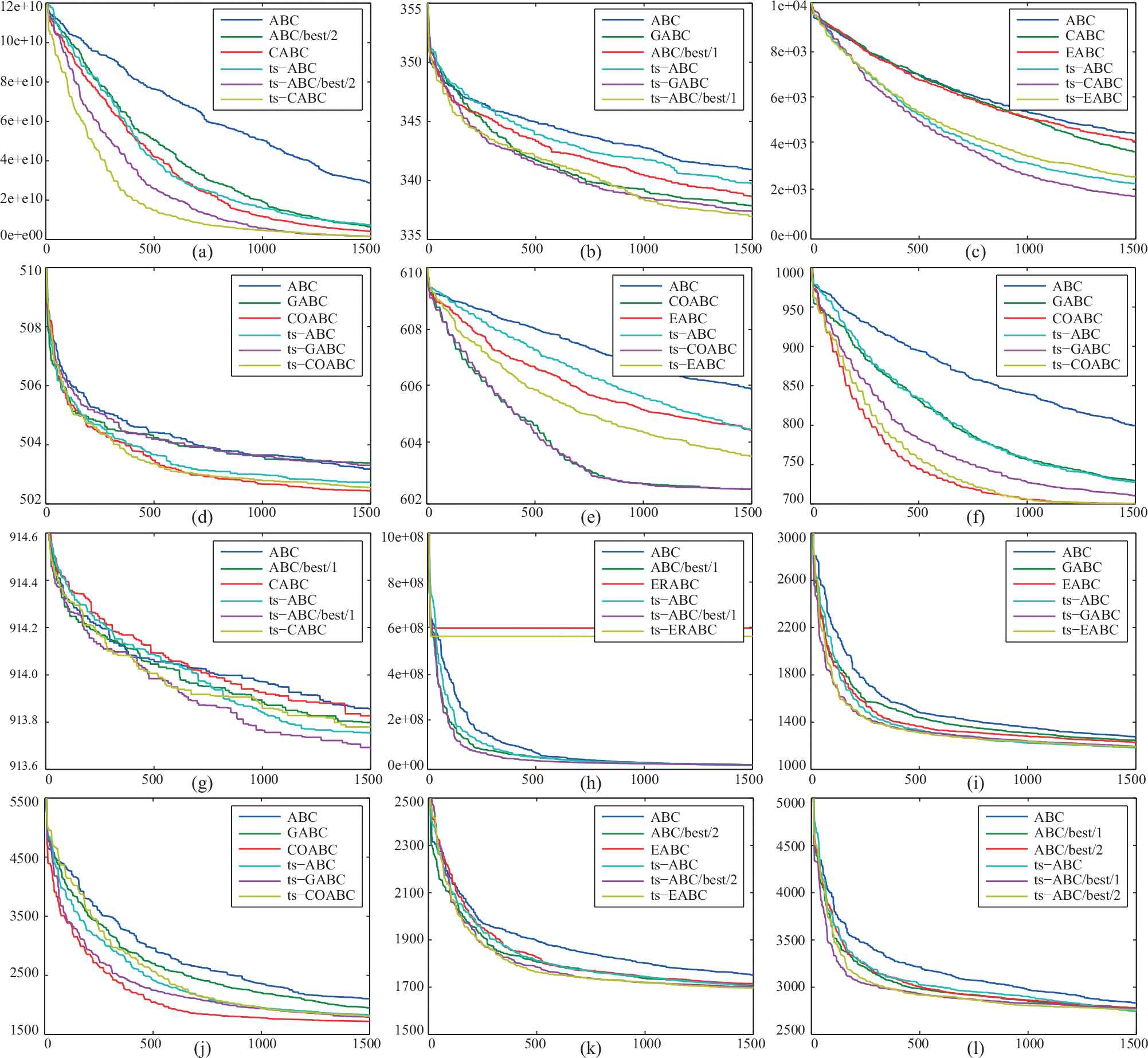
Convergence graphics of Artificial Bee Colony (ABC) algorithms for (l) functions.
Although the differences between mean best objective function values of the ABC algorithms and their ts mechanism–based variants are generally in favor of proposed models, a statistical test should also be used whether mentioned differences between variants are also meaningful or not. With this purpose, a commonly used statistical test called Wilcoxon signed rank test with the significance level
| Function | ABC vs ts-ABC | GABC vs ts-GABC | ABC/best/1 vs ts-ABC/best/1 | ABC/best/2 vs ts-ABC/best/2 | ||||
|---|---|---|---|---|---|---|---|---|
| p-val. | Sign. | p-val. | Sign. | p-val. | Sign. | p-val. | Sign. | |
| 0.000089 | ts-ABC | 0.000254 | ts-GABC | 0.001713 | ABC/best/1 | 0.000089 | ts-ABC/best/2 | |
| 0.000001 | ABC | 0.736875 | - | 0.191334 | - | 0.822760 | - | |
| 0.135357 | - | 0.575486 | - | 0.012374 | ts-ABC/best/1 | 0.601213 | - | |
| 0.000103 | ts-ABC | 0.000089 | ts-GABC | 0.000089 | ts-ABC/best/1 | 0.000103 | ts-ABC/best/2 | |
| 0.007189 | ts-ABC | 0.822760 | - | 0.940481 | - | 0.061953 | - | |
| 0.000089 | ts-ABC | 0.000103 | ts-GABC | 0.008968 | ABC/best/1 | 0.000390 | ts-ABC/best/2 | |
| 0.000120 | ts-ABC | 0.000103 | ts-GABC | 0.061953 | - | 0.000103 | ts-ABC/best/2 | |
| 0.052222 | - | 0.000780 | ts-GABC | 0.167184 | - | 0.008034 | ts-ABC/best/2 | |
| 0.145400 | - | 0.970220 | - | 0.390533 | - | 0.145400 | - | |
| 0.881293 | - | 0.654159 | - | 0.940481 | - | 0.073138 | - | |
| 0.000254 | ts-ABC | 0.027621 | ts-GABC | 0.278965 | - | 0.135357 | - | |
| 0.108427 | - | 0.145400 | - | 0.116888 | - | 0.217957 | - | |
| 0.000089 | ts-ABC | 0.000189 | ts-GABC | 0.002495 | ABC/best/1 | 0.001162 | ts-ABC/best/2 | |
| 0.003592 | ts-ABC | 0.247145 | - | 0.232226 | - | 0.204330 | - | |
| 0.040044 | ts-ABC | 0.262722 | - | 0.156004 | - | 0.247145 | - | |
| Function | COABC vs ts-COABC | CABC vs ts-CABC | ERABC vs ts-ERABC | EABC vs ts-EABC | ||||
| p-val. | Sign. | p-val. | Sign. | p-val. | Sign. | p-val. | Sign. | |
| 0.001944 | COABC | 0.001162 | ts-CABC | 0.116888 | - | 0.000254 | ts-EABC | |
| 0.940481 | - | 0.455273 | - | 0.455273 | - | 0.970220 | - | |
| 0.627446 | - | 0.036561 | ts-CABC | 0.191334 | - | 0.025094 | ts-EABC | |
| 0.004550 | - | 0.000089 | ts-CABC | 0.455273 | - | 0.000089 | ts-EABC | |
| 0.654159 | - | 0.822760 | - | 0.046222 | ts-ERABC | 0.350656 | - | |
| 0.851925 | - | 0.000517 | - | 0.204330 | - | 0.000338 | ts-EABC | |
| 0.736875 | - | 0.000089 | ts-CABC | 0.940481 | - | 0.000681 | ts-EABC | |
| 0.000293 | COABC | 0.006425 | ts-CABC | 0.135357 | - | 0.079322 | - | |
| 0.125859 | - | 0.322467 | - | 0.350656 | - | 0.881293 | - | |
| 0.204330 | - | 0.940481 | - | 0.765198 | - | 0.331723 | - | |
| 0.313463 | - | 0.100458 | - | 0.047138 | ts-ERABC | 0.018675 | ts-EABC | |
| 0.001507 | COABC | 0.708905 | - | 0.822760 | - | 0.025094 | ts-EABC | |
| 0.001162 | COABC | 0.000189 | ts-CABC | 0.473271 | - | 0.040044 | ts-EABC | |
| 0.331723 | - | 0.008034 | ts-CABC | 0.455273 | - | 0.018675 | ts-EABC | |
| 0.056661 | - | 0.331723 | - | 0.313463 | - | 1.000000 | - | |
ABC, Artificial Bee Colony; Std.Dev., standard deviation; COABC, converge-onlookers ABC; GABC, gbest-guided ABC.
Statistical comparison between ABC, GABC, ABC/best/1, ABC/best/2, COABC, CABC, ERABC, EABC algorithms, and their ts mechanism–based variants.
When the test results given in Table 10 are investigated, it is easily seen that if there is a statistical significance between ABC algorithms and their ts mechanism–based counterparts, it is usually in favor of ts mechanism–based ABC variants. The small differences between mean best objective function values of ABC, GABC, ABC/best/2, CABC, EABC algorithms and their proposed variants are enough for statistical significances that are in favor of ts-based variants at least six or more benchmark functions. For ABC/best/1 and ERABC algorithms, there are two benchmark functions for which ts mechanism–based variants are also statistically significant. Only for COABC algorithm, ts mechanism cannot be capable of generating statistically significant differences between mean best objective function values. While the differences between COABC and ts-COABC algorithms are significant in favor of COABC algorithm for
A final comparison between ABC algorithms and their ts-based variants is made over the average execution times of them. The ts mechanism requires some operations for determining initial dancing durations and controlling whether an employed bee will stay on the dance area or not. Even though mentioned ts operations bring extra burden to the total execution times of the ABC algorithms, they significantly change the selection characteristics of the onlooker bees. As mentioned before, the food source selection procedure of the ABC algorithm and its variants is managed with a randomized model. In this randomized selection model, if a random number generated between
Because of the subtle balance between computational burden of the ts mechanism and positive contribution to the selection characteristics of the onlooker bees, the average execution times of the ABC algorithms and their ts-based implementations should be found relatively close to each other. When the average execution times in terms of seconds calculated over the
| Function | ABC | ts-ABC | GABC | ts-GABC | ABC/best/1 | ts-ABC/best/1 | ABC/best/2 | ts-ABC/best/2 | |
|---|---|---|---|---|---|---|---|---|---|
| Mean | 0.050131 | 0.046639 | 0.059183 | 0.052870 | 0.041121 | 0.037392 | 0.045853 | 0.041305 | |
| Std.Dev. | 2.242718e-02 | 8.920995e-03 | 3.164774e-01 | 1.499793e-02 | 7.106844e-03 | 1.674738e-03 | 1.467020e-02 | 1.203549e-02 | |
| Mean | 0.040583 | 0.043533 | 0.054152 | 0.055728 | 0.038437 | 0.039688 | 0.049270 | 0.059717 | |
| Std.Dev. | 2.850145e-02 | 2.139360e-02 | 2.760976e-02 | 2.285981e-02 | 2.228508e-03 | 2.313789e-03 | 1.697972e-02 | 2.257493e-02 | |
| Mean | 0.672528 | 0.605529 | 0.688751 | 0.580251 | 0.460302 | 0.470560 | 0.537115 | 0.538602 | |
| Std.Dev. | 6.792684e-01 | 1.774436e-01 | 2.895477e-01 | 1.269505e-01 | 4.413920e-03 | 4.202001e-03 | 9.405997e-02 | 8.781438e-02 | |
| Mean | 0.051875 | 0.044763 | 0.041951 | 0.038930 | 0.039228 | 0.039782 | 0.048429 | 0.039847 | |
| Std.Dev. | 3.532368e-01 | 1.707656e-02 | 1.160175e-02 | 2.430201e-03 | 2.091136e-03 | 2.446647e-03 | 3.055497e-02 | 2.147554e-02 | |
| Mean | 0.429912 | 0.444856 | 0.481442 | 0.434269 | 0.350375 | 0.343755 | 0.527405 | 0.474085 | |
| Std.Dev. | 8.362566e-02 | 1.308049e-01 | 1.582201e-01 | 1.213690e-01 | 7.413277e-03 | 4.768584e-03 | 3.288734e-01 | 4.382081e-02 | |
| Mean | 0.048418 | 0.050962 | 0.055029 | 0.050854 | 0.045982 | 0.042839 | 0.040660 | 0.042495 | |
| Std.Dev. | 2.142011e-02 | 3.196463e-01 | 2.933311e-01 | 1.921920e-01 | 9.299369e-03 | 1.319572e-03 | 2.099218e-01 | 1.992233e-02 | |
| Mean | 0.081208 | 0.089252 | 0.040867 | 0.040748 | 0.048316 | 0.040513 | 0.043427 | 0.048907 | |
| Std.Dev. | 2.302384e-01 | 3.539231e-01 | 9.055348e-03 | 4.076368e-01 | 1.767417e-03 | 1.744643e-03 | 1.680284e-02 | 2.096029e-02 | |
| Mean | 0.058148 | 0.049594 | 0.054278 | 0.069050 | 0.035208 | 0.035991 | 0.092171 | 0.101456 | |
| Std.Dev. | 2.455125e-01 | 5.855726e-03 | 2.699446e-02 | 4.720703e-01 | 1.964160e-03 | 2.021030e-03 | 3.344670e-01 | 3.038753e-01 | |
| Mean | 0.063104 | 0.068442 | 0.058388 | 0.060236 | 0.046402 | 0.037682 | 0.059763 | 0.052081 | |
| Std.Dev. | 1.969610e-02 | 4.969772e-03 | 1.549435e-02 | 3.713047e-02 | 1.967376e-03 | 1.080150e-03 | 2.270765e-01 | 5.650666e-03 | |
| Mean | 0.105905 | 0.092958 | 0.068589 | 0.078626 | 0.048444 | 0.439376 | 0.058933 | 0.050908 | |
| Std.Dev. | 4.294203e-01 | 9.130607e-02 | 1.245935e-01 | 5.811356e-01 | 2.310650e-03 | 1.915442e-03 | 2.997234e-02 | 1.240162e-02 | |
| Mean | 0.157163 | 0.156823 | 0.167664 | 0.166312 | 0.125320 | 0.127797 | 0.154117 | 0.132302 | |
| Std.Dev. | 5.415421e-02 | 3.213212e-02 | 5.846262e-02 | 1.720524e-01 | 2.689619e-03 | 2.909550e-03 | 2.592682e-02 | 1.362776e-02 | |
| Mean | 0.091845 | 0.095219 | 0.102071 | 0.125829 | 0.072141 | 0.074464 | 0.130435 | 0.079509 | |
| Std.Dev. | 1.658417e-02 | 2.953888e-02 | 2.345862e-02 | 2.097525e-01 | 2.735565e-03 | 2.963951e-03 | 5.064997e-02 | 9.973386e-03 | |
| Mean | 0.122911 | 0.114850 | 0.133987 | 0.109591 | 0.097796 | 0.097495 | 0.153980 | 0.173686 | |
| Std.Dev. | 3.385718e-02 | 1.539274e-02 | 7.096232e-02 | 1.404100e-02 | 1.880880e-03 | 2.222095e-03 | 7.549713e-01 | 2.580564e-01 | |
| Mean | 0.149240 | 0.120973 | 0.122755 | 0.143693 | 0.091375 | 0.093722 | 0.107004 | 0.131532 | |
| Std.Dev. | 6.229411e-02 | 1.193391e-02 | 5.597142e-01 | 5.455718e-02 | 2.973894e-03 | 1.123502e-02 | 2.603938e-02 | 3.791140e-01 | |
| Mean | 0.602323 | 0.642129 | 0.652188 | 0.678815 | 0.544688 | 0.549962 | 0.643163 | 0.779873 | |
| Std.Dev. | 8.578987e-02 | 7.396672e-02 | 6.492040e-02 | 1.706552e-01 | 5.006217e-03 | 7.031245e-03 | 1.224565e-01 | 3.356357e-01 | |
ABC, Artificial Bee Colony; Std.Dev., standard deviation; GABC, gbest-guided ABC.
Average execution times of ABC, GABC, ABC/best/1, ABC/best/2 algorithms, and their ts mechanism–based variants.
| Function | COABC | ts-COABC | CABC | ts-CABC | ERABC | ts-ERABC | EABC | ts-EABC | |
|---|---|---|---|---|---|---|---|---|---|
| Mean | 0.065230 | 0.066156 | 0.048353 | 0.056149 | 0.046515 | 0.062363 | 0.042773 | 0.049179 | |
| Std.Dev. | 2.297517e-02 | 1.652955e-01 | 2.492893e-03 | 1.890919e-02 | 2.339866e-03 | 2.313109e-02 | 1.500081e-02 | 2.101563e-03 | |
| Mean | 0.048287 | 0.048671 | 0.047731 | 0.049990 | 0.046675 | 0.051666 | 0.045216 | 0.049033 | |
| Std.Dev. | 3.843406e-03 | 1.226867e-02 | 2.183988e-03 | 8.376007e-03 | 2.372530e-03 | 4.363600e-01 | 1.527630e-02 | 1.714590e-03 | |
| Mean | 0.642305 | 0.625817 | 0.464593 | 0.572149 | 0.467411 | 0.600064 | 0.655932 | 0.569024 | |
| Std.Dev. | 2.020452e-01 | 1.927304e-01 | 4.733351e-03 | 3.458033e-01 | 3.271359e-02 | 1.275539e-01 | 3.551220e-01 | 4.200882e-03 | |
| Mean | 0.052991 | 0.052837 | 0.049458 | 0.046331 | 0.048568 | 0.053026 | 0.044320 | 0.049970 | |
| Std.Dev. | 2.889452e-01 | 5.392231e-02 | 3.156447e-03 | 5.992266e-03 | 2.107408e-03 | 3.019394e-02 | 1.609946e-02 | 2.027419e-03 | |
| Mean | 0.486031 | 0.476229 | 0.554044 | 0.605130 | 0.547858 | 0.502536 | 0.494557 | 0.446165 | |
| Std.Dev. | 1.748296e-01 | 1.440274e-01 | 4.264174e-03 | 1.997422e-01 | 3.356789e-03 | 2.664092e-01 | 5.522459e-02 | 3.541961e-03 | |
| Mean | 0.054199 | 0.057993 | 0.069152 | 0.077372 | 0.047787 | 0.057286 | 0.044491 | 0.049964 | |
| Std.Dev. | 1.289931e-02 | 3.290299e-01 | 2.164248e-03 | 3.150003e-02 | 2.288113e-03 | 2.577948e-02 | 8.064113e-03 | 2.112660e-03 | |
| Mean | 0.058557 | 0.056617 | 0.049679 | 0.042025 | 0.039372 | 0.041644 | 0.036487 | 0.039817 | |
| Std.Dev. | 2.450032e-01 | 5.599165e-03 | 2.488866e-03 | 1.175164e-02 | 2.025220e-03 | 1.466875e-02 | 8.675390e-03 | 2.522923e-03 | |
| Mean | 0.059404 | 0.061252 | 0.044772 | 0.053283 | 0.044144 | 0.053763 | 0.054268 | 0.047425 | |
| Std.Dev. | 1.448049e-02 | 1.587708e-02 | 1.555508e-03 | 1.514707e-02 | 1.105658e-02 | 1.421387e-02 | 1.502297e-02 | 2.056765e-03 | |
| Mean | 0.042446 | 0.042979 | 0.045441 | 0.053175 | 0.044930 | 0.497018 | 0.067967 | 0.057086 | |
| Std.Dev. | 5.893791e-03 | 5.309384e-02 | 1.960864e-03 | 3.008490e-02 | 1.662135e-03 | 7.127754e-01 | 3.304973e-02 | 1.971332e-03 | |
| Mean | 0.058155 | 0.062264 | 0.068542 | 0.063555 | 0.050538 | 0.065660 | 0.047023 | 0.050844 | |
| Std.Dev. | 6.084131e-02 | 5.452598e-01 | 1.812356e-03 | 1.795279e-02 | 1.400168e-02 | 1.137388e-01 | 3.423352e-01 | 1.532782e-03 | |
| Mean | 0.144628 | 0.170425 | 0.124703 | 0.168718 | 0.124929 | 0.166217 | 0.128905 | 0.136100 | |
| Std.Dev. | 4.635860e-02 | 4.743490e-02 | 2.834806e-03 | 6.327066e-02 | 3.438445e-03 | 5.829321e-02 | 4.551299e-01 | 2.603739e-03 | |
| Mean | 0.102036 | 0.072304 | 0.072711 | 0.190395 | 0.072076 | 0.100883 | 0.102415 | 0.073278 | |
| Std.Dev. | 3.555396e-02 | 1.879055e-02 | 3.500502e-03 | 1.618380e-01 | 2.611370e-03 | 2.088056e-02 | 3.048965e-02 | 3.004425e-03 | |
| Mean | 0.183922 | 0.158835 | 0.096309 | 0.115690 | 0.095778 | 0.113198 | 0.134287 | 0.149578 | |
| Std.Dev. | 5.134852e-01 | 4.997218e-02 | 1.729511e-03 | 1.395025e-02 | 2.479506e-03 | 5.187983e-02 | 4.515653e-02 | 3.588585e-03 | |
| Mean | 0.104493 | 0.099019 | 0.093205 | 0.113302 | 0.090379 | 0.117564 | 0.107687 | 0.090693 | |
| Std.Dev. | 2.118410e-02 | 1.433848e-02 | 4.081801e-03 | 2.379353e-01 | 1.796991e-03 | 4.278472e-01 | 2.656273e-02 | 2.370891e-03 | |
| Mean | 0.687970 | 0.601772 | 0.557062 | 0.662383 | 0.552846 | 0.630580 | 0.611085 | 0.550082 | |
| Std.Dev. | 1.955580e-01 | 5.276792e-02 | 3.366157e-03 | 3.250891e-01 | 4.767583e-02 | 8.352474e-02 | 2.777474e-01 | 8.321810e-03 | |
ABC, Artificial Bee Colony; Std.Dev., standard deviation; COABC, converge-onlookers ABC.
Average execution times of COABC, CABC, ERABC, EABC algorithms, and their ts mechanism–based variants.
5. CONCLUSION
In this study, dancing characteristics of the employed bees are modeled with a new approach called time-based dance scheduling for short ts mechanism. The ts mechanism is integrated to the standard ABC algorithm and its well-known variants. Experimental studies on a set of difficult benchmark problems showed that standard ABC algorithm and its variants especially those require selection of the food source being consumed and the neighbor food source or sources being utilized are improved with the proposed mechanism in terms of qualities of the solutions and convergence speeds.
The improvements with the ts mechanism also provide important information about the possible contributions of the unmodeled forager characteristics. Some bee characteristics that are not directly included in the standard ABC algorithm or related with the randomized operations can be integrated to the workflow of the algorithm for increasing the performance and reflecting the intelligent behaviours more completely. In future, ABC algorithm can be modified by modeling decision-making characteristics of the employed foragers that is used whether or not an employed forager is transitioned to the dance area or different timing mechanisms in which the start and finish times of dancing are determined according to the qualities of the memorized sources.
References
Cite this article
TY  - JOUR
AU  - Selcuk Aslan
PY  - 2019
DA  - 2019/05/11
TI  - Time-Based Dance Scheduling for Artificial Bee Colony Algorithm and Its Variants
JO  - International Journal of Computational Intelligence Systems
SP  - 597
EP  - 612
VL  - 12
IS  - 2
SN  - 1875-6883
UR  - https://doi.org/10.2991/ijcis.d.190425.001
DO  - 10.2991/ijcis.d.190425.001
ID  - Aslan2019
ER  -