
Multi-Attribute Decision-Making Method Based on Prospect Theory in Heterogeneous Information Environment and Its Application in Typhoon Disaster Assessment
- DOI
- 10.2991/ijcis.d.190722.002How to use a DOI?
- Keywords
- Multi-attribute decision-making (MADM); Heterogeneous information; Prospect theory; Neutrosophic set; Typhoon disaster assessment
- Abstract
Aiming at the decision-making problem in heterogeneous information environment and considering the influence of decision makers' psychological behavior on decision-making results, this paper proposes a multi-attribute decision-making method based on prospect theory in heterogeneous information environment. The heterogeneous information in this paper indicates that the decision attribute value is represented by various types of data forms, including exact number, interval number, linguistic term, intuitionistic fuzzy number, interval intuitionistic fuzzy number, neutrosophic numbers, and trapezoidal fuzzy neutrosophic numbers, and so on. Firstly, the distance and similarity measure of various heterogeneous data are introduced, and the heterogeneous information attribute weights are obtained using the deviation maximization method. Then, the psychological expectation value of each attribute given by the decision maker is used as a reference point, thereby calculating the gain and loss of each attribute value relative to the reference point, and establishing a gain matrix and a loss matrix. On this basis, the prospect theory is used to obtain the comprehensive prospect value of each alternative, so as to obtain the alternative ordering result and optimal alternative. Finally, an illustrative example about typhoon disaster assessment is presented to show the feasibility and effectiveness of the proposed method, and the advantages of the proposed method are illustrated by comparison with other methods.
- Copyright
- © 2019 The Authors. Published by Atlantis Press SARL.
- Open Access
- This is an open access article distributed under the CC BY-NC 4.0 license (http://creativecommons.org/licenses/by-nc/4.0/).
1. INTRODUCTION
Multi-attribute decision-making is a problem in which a decision-maker evaluates a finite set of alternatives associated with multiple attributes [1]. It has been widely applied in many practical problems, such as supplier selection [2,3], pattern recognition [4], medical diagnosis [5,6], emergency decision [7,8], water allocation [9], disaster assessment [10–12], and so on. Therefore, the multi-attribute decision-making method has become the focus of scholars and has been extensively studied. However, the decision-making problem has become more and more complicated because of the increasing amount of decision information and alternatives, and the inherent uncertainty and complexity of decision problems, and the fuzzy nature of human thinking [12]. Especially in some sudden, complicated situations, some decision information is often not accurately represented, often expressed as fuzzy, vague, hesitant, incomplete, indeterminate, and inconsistent. So the fuzzy set (FS) [13], hesitant fuzzy set (HFS) [14], rough set [15], grey theory [16], intuitionistic fuzzy set (IFS) [17], and neutrosophic set (NS) [18] are used to model the decision information. Throughout the existing research literature, most of the multi-attribute decision-making methods are based on a single type of data, and there are few studies on multiple data types. However, in some complicated situations, the decision is faced with heterogeneous data. For example, in our typhoon disaster assessment study, the representation of the assessment information is diverse. The number of population death is usually accurately obtained, which is expressed as an exact number (EN). The number of population affected can usually obtain its approximate range, which can be expressed as an interval number. Again, the severity of economic loss tends to be expressed in linguistic terms (LTS). If the assessment of traffic flow after disaster can get the maximum possible range and possible fluctuation range, TrFNNs can be generally used.
Heterogeneity indicates that the type and nature of information or data is different [19]. In view of the high risk, complexity, and ambiguity of typhoon disasters, evaluation information cannot always be expressed as ENs, and often has the characteristics of interval, ambiguity, and hesitation, and is more appropriately expressed as interval numbers (IVNs), fuzzy numbers (FNs), and intuitionistic fuzzy numbers (IFNs). In addition, due to the ambiguity of human thinking, it is difficult to use the quantitative numerical representation of decision information in the decision-making process, and it is more inclined to use qualitative LTs to evaluate attributes. At the same time, typhoon disasters also have great uncertainty. Such evaluation information can be characterized as neutrosophic numbers (NNs), trapezoidal fuzzy neutrosophic numbers (TrFNNs), and so on. So, the processing heterogeneous information is a key point in the decision-making process [1,19–21]. Sun et al. [1] proposed a MADM with grey multi-source heterogeneous data including ENs, interval grey numbers, and extend grey numbers. Yu et al. [19] proposed a heterogeneous MADM considering four types of data: ENs, IVNs, triangular fuzzy numbers (TFNs), and IFNs. Pan et al. [20] proposed a hybrid MADM based on VIKOR with multi-granularity LNs, ENs, IVNs. Wan et al. [21] proposed a MADM for heterogeneous infromation including ENs, IVNs, TFNs, and trapezoidal fuzzy numbers (TrFNs). Lourenzutti et al. [22] proposed a generalized TOPSIS method for MADM with heterogeneous information including crisp numbers, IVNs, FNs, IFNs, and random vectors. Zhang et al. [23] proposed a risk-based MADM based on three heterogeneous data: ENs, IVNs, and TFNs. Fanet et al. [24] proposed a hybrid MADM based on cumulative prospect theory (PT) with heterogeneous data including ENs, IVNs, and LTs. Qi et al. [25] proposed a MADM based on heterogeneous data such as multi-granularity language numbers, IFNs, and interval intuitionistic fuzzy numbers (IVIFNs) into IVIFNs to calculate the comprehensive evaluation value of the alternative. However, looking at the existing research literature, we have not seen the study of heterogeneous data including the NN. On the other hand, in terms of practical applications, the assessment of post-typhoon disasters is a very complicated issue, and it is sometimes difficult for experts to make clear decisions. For example, we invited the expert group to assess the severity of social impact, 30% vote “Yes,” 20% vote “No,” 10% give up, and 40% are undecided. Such a vote is beyond the scope of IFS to distinguish the information between “giving up” and “undecided.” Such a scenario indicates that the NN needs to be studied in depth. Therefore, we studies the MADMs in heterogeneous information environment including the ENs, IVNs, LTs, IFNs, IVIFNs, NNs, and TrFNNs, and so on.
NSs proposed by Smarandache [26] are a powerful tool to deal with incomplete, indeterminate, and inconsistent information in the real world. And it is the generalization of the theory of FSs [13], interval-valued fuzzy sets, and IFSs [17], and so on. NSs are characterized by a truth-membership degree (T), an indeterminacy-membership degree (I), and a falsity-membership degree (F), which can represent more information than other FSs. In recent years, scholars have proposed various forms of NNs. For example, Wang et al. [27] introduced the concept of single-valued neutrosophic sets (SVNSs). Ye [28] introduced the simplified neutrosophic sets (SNSs). SVNS is an extension of FN and IFN. Wang and Li [29] also defined multi-valued neutrosophic sets (MVNSs). Wang et al. [30] proposed interval neutrosophic sets (INSs). Yang and Pang [31] defined multi-valued interval neutrosophic sets (MVINSs). Deli et al. [32] proposed the concept of the bipolar NSs, and applied it to MADM. Deli et al. proposed neutrosophic refined sets [33] and bipolar neutrosophic refined sets [34] and applied them to medical diagnosis. Tian et al. [35] proposed the concept of the simplified neutrosophic linguistic and applied it to MADM. Broumi et al. [36–38] and Tan et al. [39] combined the NSs and graph theory to propose neutrosophic graphs, and used for the shortest path solving problem. Ye [40] proposed trapezoidal fuzzy NSs and applied them to MADM. There are many forms of NN, which are suitable for different decision-making environments. The heterogeneous data of typhoon disaster assessment we studied include single-valued neutrosophic numbers (SVNNs) and TrFNN.
Sorting method is a research hotspot in decision-making including method based on scoring function and exact function, similarity measure method, VIKOR method, TOPSIS method, grey theory, TODIM method, and so on, and most of the methods are based on the assumption that the decision maker is completely rational. But some studies about behavioral experiments have shown that the decision maker is bounded rational in decision processes and his behavior plays an important role in decision analysis [41]. In the face of emergencies, especially after the disaster, the psychological factors of decision makers play a key role in decision-making, and the research on this aspect is still rare. PT introduced by Kahneman et al. [42,43] provides a simple and clear computation process to describe the psychological behavior using reference points, losses, gains, and overall prospect values [44]. So it has been widely applied in the various fields to solve the practical problems considering human being's psychological behavior. Gao et al. [45] and Best et al. [46] applied PT to solve asset allocation. Attema et al. [47] studied the application of PT in the field of health domains. Tian et al. [48] studied the park-and-ride behavior in a cumulative PT-based model. Van Tol et al. [49] studied the application of cumulative PT in option valuation and portfolio management. Zou et al. [50] studied the optimal investment with transaction costs under cumulative PT. Liu et al. [51] and Zhang et al. [52] proposed emergency decision-making methods based on PT. Tao et al. [53] proposed the brain mechanism of economic management risk decision based on PT. Ning et al. [54] studied the disruption management strategy based on PT. Sullivan et al. [55] examined the forest certification problem based on PT. Yu et al. [56] studied the typhoon disaster emergency scheme generation and dynamic adjustment based on CBR and PT. However, given the existing research, there is still little literature on the application of PT in typhoon disaster assessment. Taking into account the uncertainty of typhoon disasters and the psychological feelings of decision makers, the PT can well consider the psychological factors of decision makers to the assessment of typhoon disasters, which can make disaster assessment more reasonable and effective. So, this paper studies typhoon disaster assessment based on PT.
Natural disasters often lead to death and enormous property damage. Various types of natural disasters occur in China every year. And the typhoon is one of the biggest disasters facing humanity. Its destructive power exceeds that of the earthquake, but it has never been avoided. Meteorological disasters such as typhoon accounted for more than 70% of the natural disasters [57]. In China, typhoons primarily impact the eastern coastal regions of the country, where the population is extremely dense, the economy is highly developed, and social wealth is notably concentrated. Once the typhoon comes, it will cause huge property and economic losses, casualties, and environmental damage to this area. Therefore, typhoon disaster assessment is a very important issue. However, the influencing factors of the typhoon disasters are completely hard to describe accurately. Taking economic loss, for example, it includes many aspects such as the building's collapse, the number and extent of damage to housing, and the affected local economic conditions [10], the degree of environmental damage, and the negative impact on society. The evaluation information is often hesitant, ambiguous, incomplete, inconsistent, indeterminate, and so on. Therefore, FSs, HFSs, and IFSs have been used for typhoon disaster assessment in recent years. For example, Shi et al. [57] proposed a fuzzy MADM hybrid approach to evaluate the damage level of typhoon based on FNs. He et al. [11] proposed a typhoon disaster assessment method based on Dombi HFNs. Li et al. [58] and Yu [10] proposed evaluating typhoon disasters method based on IFNs. Throughout the existing literature, most of the typhoon disaster assessment studies are based on a single data form, and have not yet been conducted under heterogeneous data environment containing the NNs. We believe that NS will be a powerful theory and method to enhance typhoon disaster assessment. So we study the MADM based on PT in heterogeneous information environment and apply it to the typhoon disaster assessment. First we use the deviation maximization method based on heterogeneous information to get the evaluation index weights, then use the extended PT to calculate the overall prospect value of each alternative to sort the alternatives in a heterogeneous information environment.
This paper is organized as the following: Section 2 briefly presents some basic definitions of heterogeneous information. Section 3 gives the distance formula and similarity measure of various heterogeneous data, a MADM method based on the PT, and the compatibility and consistency measures for heterogeneous information. Section 4 uses a typhoon disaster evaluation example to illustrate the applicability of the proposed method and verifies the advantages of the proposed method by comparative analysis. Finally, Section 5 gives the conclusions.
2. PRELIMINARIES
In this section, we briefly introduce the basic concepts of various heterogeneous data used in this paper, including the NNs, IFNs, FNs, ENs, and so on. At the same time, PT will be briefly reviewed so that unfamiliar readers can understand our proposed method easily.
2.1. SVNN, Trapezoidal Fuzzy NN
Definition 1.
[27] Let
Definition 2.
[40] Let
For simplicity of calculation, a TrFNN
2.2. IFNs, IVIFNs, and Interval Numbers
Definition 3.
[17] Let a set
Definition 4.
[59] An interval-valued intuitionistic fuzzy set (IVIFS)
For convenience, we can use
2.3. Language Term
Definition 5.
[60,61]: Let
In these cases, it is usually required that there exist the following:
A negation operator:
The set is ordered:
Maximum operator:
Minimum operator:
In order to preserve all the given information, extending the discrete term set
The so-called different granularity language information refers to the preference information given by the decision makers in the group decision-making according to the language evaluation set represented by the granularity of the number of different language phrases. Let
2.4. Prospect Theory
PT is a theory that describes and predicts behaviors that are inconsistent with traditional expectations theory and expected utility theory in the face of risk decision-making. The theory finds that people's risk preference behaviors are inconsistent in the face of gains and losses, and they become risk-seeking in the face of “missing,” but they are risk-averse in the face of “getting.” The establishment and change of reference points affect people's feelings of gain and loss, and thus influence people's decision-making.
In MADM problems, the attributes can be classified into two types: benefits and costs. The higher a benefit attribute is, the better the situation is, while the higher a cost attribute is, the worse the situation is. According to different types of attributes, reference points changes with people's expectations with respect to the predefined amounts to gain or lose [62]. For example, if there is a possibility to lose some money and predefined amounts are USD 5, 10 and 20, then assuming that 10 is an acceptable loss amount to an individual (reference point of possible losses), if the final outcome is 5, he/she feels gains because the final losses are lower than his/her expectation. Benefit attributes can be assessed in a similar way [52].
Gains and losses are determined by the reference point and the final outcome with respect to different types of attributes. For measuring the magnitude of gains and losses, an S-shaped value function is provided in PT [42]. The value function is expressed in the form of a power law [42]:
3. DECISION-MAKING METHOD BASED ON HETEROGENEOUS INFORMATION AND PT
3.1. Distance Measure of Heterogeneous Information
The basic idea of PT is to first use the expectation of the decision maker as a reference point, and establish the risk return matrix and the risk loss matrix, respectively, by calculating the gain and loss of the program attribute value relative to the reference point, and then to establish the prospect decision matrix. On this basis, the alternatives are ranked by calculating the comprehensive prospect values of each alternative. In the disaster assessment, after the typhoon disaster occurs, the decision makers will form a certain psychological expectation according to the report of the relevant personnel and their own situation, also known as the psychological reference point. At the same time, the degree of disaster of each assessment object is compared with the psychological reference point of the decision maker to judge the extent to which the decision maker's psychological perception is “gain” or “loss.” Among them, the calculation of the gain and loss mainly involves the distance calculation of various heterogeneous information.
Let
When the attribute value is an EN, its distance
When the attribute value is an IVN, that is
When the attribute value is an IFN, that is,
When the attribute value is a language term, that is,
where,When the attribute value is an IVIFN, that is,
When the attribute value is a NN, that is,
When the attribute value is a TrFNN, that is,
3.2. Determination of Attribute Weights in Heterogeneous Information Environment
For the objective of decision-making, this paper uses the method of maximizing deviations to calculate the attribute weights. Due to the complexity of objective things and the ambiguity of human thinking, it is often difficult to give explicit attribute weights. Sometimes there is an extreme situation where the weight is completely unknown. In the multi-attribute decision-making (MADM) of the finite alternatives, the smaller the difference of the alternative under the attribute
The weight vector
3.3. MADM Method Based on Heterogeneous Information and PT
3.3.1. Problem description and method steps
This section introduces a novel MADM method based on heterogeneous information and PT that considers decision makers' psychological behavior and deals with different types of assessment information. To achieve our objectives, the proposed method consists of the following several phases, depicted graphically in Figure 1.
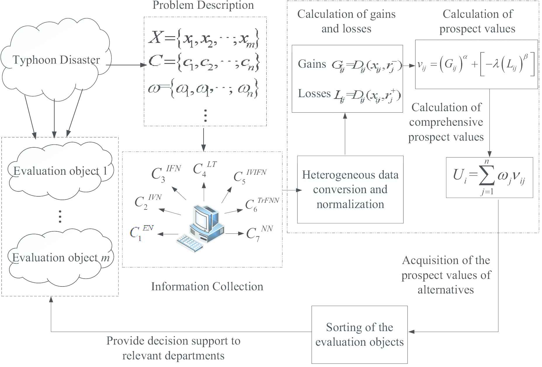
Framework of the proposed multi-attribute decision making (MADM) based on heterogeneous information and prospect theory.
Consider a MADM problem, let
Step 1: Collect heterogeneous data and get the evaluation matrix
Step 2: Get the normalized evaluation matrix
Step 3: Determine the reference point. Reference point represents the psychological expectations of decision makers for certain evaluation attributes after typhoon disasters. In order to eliminate the subjective influence of the decision maker as much as possible, this paper uses the positive and negative points of each attribute as the reference point. Positive and negative ideal solutions represent the decision makers' maximum and minimum prediction of the disaster extent of the assessed objects. So, for
Step 4: Calculate the gains and losses. Based on the gain value and the loss value, a gain matrix
Step 5: Calculation of prospect values. According to PT, the magnitude of gains and losses is measured by value function. Let
The prospect values indicate the earned value of each evaluation object for each evaluation attribute based on the decision-maker's psychological reference point. In the assessment of the typhoon disaster, they indicate the severity of the evaluation objects in a certain aspect.
Step 6: Calculate the weights and calculate the attribute weights of the heterogeneous information using Equation (13).
Step 7: The comprehensive prospect value
3.3.2. The compatibility and consistency of heterogeneous information
Measuring the level of consistency of different opinions of experts in group decision-making is a key issue. The consistency problem mainly includes two types: the consistency of the judgment matrix given by each expert and the consistency of the preference relationship between experts. Related to our research is the latter, which is the compatibility and consistency of information in group decision-making. When a group of decision-makers' preference relationships are similar, there is consistency among decision makers. In the absence of basic compatibility, unsatisfactory or incorrect results may result in group decision problems, and the evaluation information needs to be adjusted. The research on the compatibility and consistency of information including uncertain information has yielded rich results [73–75], but there are not many related researches on heterogeneous information, especially including NNs. We have been inspired by the literature [73] to propose the judgment method and adjustment strategy of compatibility and consistency for heterogeneous information are as follows:
Step 1: We first convert the multiple evaluation matrices
Step 2: We use the TNNWAA operator to assemble the group evaluation matrices into a comprehensive evaluation matrix
Step 3: We calculate the compatibility index
Step 4: We predetermine the critical value
Step 5: If there is an expert evaluation matrix
In particular, we only give compatibility and consistency judgment methods and adjustment strategies for heterogeneous information, and our case study section does not make specific calculations.
4. CASE STUDY AND COMPARISON WITH OTHER APPROACHES
4.1. Case Study
With the rapid development of China's economy and the growing development of coastal cities, the losses caused by typhoon disasters have become increasingly serious. Take Fujian Province as an example. It is located in the southeast coastal area of China. It is close to the typhoon source and is on the path of typhoon movement. Typhoon is often landed. When the typhoon landed, it brought disasters such as storms and storm surges. Therefore, this paper evaluates the typhoon disasters in Fujian Province. Taking a strong typhoon “Maria” in Fujian Province in July 2018 as an example, “Maria” landed on the coast of Lianjiang River at 9:10 on November 11. When landing, the maximum wind force near the center was 14 levels (42/sec, strong typhoon level), and the lowest central pressure was 960 hPa. It was the strongest typhoon landing in Fujian since July with meteorological records. It was strong, fast moving, and destructive. After the disaster, we quickly obtains heterogeneous data from multiple sources for disaster assessment, which provides decision support for disaster relief in relevant departments. This paper synthesizes the literature [56] and [10] to construct an assessment indicator system. The assessment indicators
| Index |
||||
|---|---|---|---|---|
| Cities | c1 | c2 | c3 | c4 |
| Nanping (NP) | 3 | [2,100–200,000] | ||
| Ningde (ND) | 10 | [65,000–1,900,000] | ||
| Sanming (SM) | 2 | [2,000–190,000] | ||
| Fuzhou (FZ) | 7 | [180,000–600,000] | ||
| Putian(PT) | 5 | [1,000,000–2,000,000] | ||
| Longyan (LY) | 3 | [5,000–300,000] | ||
| Quanzhou (QZ) | 4 | [18,000–500,000] | ||
| Xiamen (XM) | 3 | [2,300–190,000] | ||
| Zhangzhou (ZZ) | 6 | [500,000–2,000,000] |
| Index |
|||
|---|---|---|---|
| Cities | c5 | c6 | c7 |
| Nanping (NP) | |||
| Ningde (ND) | |||
| Sanming (SM) | |||
| Fuzhou (FZ) | |||
| Putian (PT) | |||
| Longyan (LY) | |||
| Quanzhou (QZ) | |||
| Xiamen (XM) | |||
| Zhangzhou (ZZ) |
Evaluation Matrix R.
Step 1: For the convenience of calculation, the language term is converted into IVIFN according to the literature [25], and the transformed data is shown in Table 2.
| Index |
||||
|---|---|---|---|---|
| Cities | c1 | c2 | c3 | c4 |
| Nanping (NP) | 3 | [2,100–200,000] | ||
| Ningde (ND) | 10 | [65,000–1,900,000] | ||
| Sanming (SM) | 2 | [2,000–190,000] | ||
| Fuzhou (FZ) | 7 | [180,000–600,000] | ||
| Putian (PT) | 5 | [1,000,000–2,000,000] | ||
| Longyan (LY) | 3 | [5,000–300,000] | ||
| Quanzhou (QZ) | 4 | [18,000–500,000] | ||
| Xiamen (XM) | 3 | [2,300–190,000] | ||
| Zhangzhou (ZZ) | 6 | [500,000–2,000,000] |
Converted evaluation matrix R.
Step 2: We use Equation (14) to get the normalized evaluation matrix
| Index |
||||
|---|---|---|---|---|
| Cities | c1 | c2 | c3 | c4 |
| Nanping (NP) | 0.300 | [0.001, 0.100] | ||
| Ningde (ND) | 1.000 | [0.033, 0.950] | ||
| Sanming (SM) | 0.200 | [0.001, 0.095] | ||
| Fuzhou (FZ) | 0.700 | [0.090, 0.300] | ||
| Putian (PT) | 0.500 | [0.500, 1.000] | ||
| Longyan (LY) | 0.300 | [0.003, 0.150] | ||
| Quanzhou (QZ) | 0.400 | [0.009, 0.250] | ||
| Xiamen (XM) | 0.300 | [0.012, 0.095] | ||
| Zhangzhou (ZZ) | 0.600 | [0.250, 1.000] |
| Index |
|||
|---|---|---|---|
| Cities | c5 | c6 | c7 |
| Nanping (NP) | |||
| Ningde (ND) | |||
| Sanming (SM) | |||
| Fuzhou (FZ) | |||
| Putian (PT) | |||
| Longyan (LY) | |||
| Quanzhou (QZ) | |||
| Xiamen (XM) | |||
| Zhangzhou (ZZ) |
Normalized evaluation matrix
Step 3: Determine the reference point. For
Step 4: Calculate the gains and losses to get the gain matrix
| Index |
|||||||
|---|---|---|---|---|---|---|---|
| Cities | c1 | c2 | c3 | c4 | c5 | c6 | c7 |
| Nanping (NP) | 0.583 | 0.631 | 0.889 | 0.633 | 0.499 | 0.618 | 0.722 |
| Ningde (ND) | 0.000 | 0.365 | 0.008 | 0.000 | 0.000 | 0.000 | 0.484 |
| Sanming (SM) | 0.632 | 0.632 | 0.889 | 0.633 | 0.499 | 0.618 | 0.810 |
| Fuzhou (FZ) | 0.313 | 0.544 | 0.221 | 0.039 | 0.216 | 0.232 | 0.185 |
| Putian (PT) | 0.465 | 0.000 | 0.008 | 0.112 | 0.096 | 0.027 | 0.253 |
| Longyan (LY) | 0.583 | 0.614 | 0.761 | 0.280 | 0.301 | 0.483 | 0.620 |
| Quanzhou (QZ) | 0.528 | 0.580 | 0.889 | 0.483 | 0.499 | 0.232 | 0.087 |
| Xiamen (XM) | 0.583 | 0.630 | 0.531 | 0.582 | 0.421 | 0.483 | 0.000 |
| Zhangzhou (ZZ) | 0.393 | 0.215 | 0.000 | 0.039 | 0.000 | 0.232 | 0.185 |
Loss matrix LM.
| Index |
|||||||
|---|---|---|---|---|---|---|---|
| Cities | c1 | c2 | c3 | c4 | c5 | c6 | c7 |
| Nanping (NP) | 0.118 | 0.005 | 0.000 | 0.032 | 0.000 | 0.000 | 0.089 |
| Ningde (ND) | 0.632 | 0.563 | 0.761 | 0.633 | 0.499 | 0.618 | 0.339 |
| Sanming (SM) | 0.000 | 0.000 | 0.000 | 0.032 | 0.000 | 0.000 | 0.000 |
| Fuzhou (FZ) | 0.465 | 0.194 | 0.291 | 0.594 | 0.289 | 0.128 | 0.630 |
| Putian (PT) | 0.313 | 0.632 | 0.761 | 0.523 | 0.404 | 0.438 | 0.563 |
| Longyan (LY) | 0.118 | 0.052 | 0.008 | 0.356 | 0.204 | 0.019 | 0.195 |
| Quanzhou (QZ) | 0.221 | 0.139 | 0.000 | 0.153 | 0.000 | 0.128 | 0.729 |
| Xiamen (XM) | 0.118 | 0.011 | 0.070 | 0.055 | 0.082 | 0.019 | 0.810 |
| Zhangzhou (ZZ) | 0.393 | 0.597 | 0.889 | 0.594 | 0.499 | 0.128 | 0.630 |
Gain matrix GM.
Step 5: Using Equation (15) to calculation of prospect values when
| Index |
|||||||
|---|---|---|---|---|---|---|---|
| Cities | c1 | c2 | c3 | c4 | c5 | c6 | c7 |
| Nanping (NP) | −1.220 | −1.464 | −2.019 | −1.431 | −1.187 | −1.445 | −1.551 |
| Ningde (ND) | 0.665 | −0.290 | 0.758 | 0.666 | 0.539 | 0.652 | −0.772 |
| Sanming (SM) | −1.475 | −1.475 | −2.019 | −1.431 | −1.187 | −1.445 | −1.853 |
| Fuzhou (FZ) | −0.267 | −1.053 | −0.228 | 0.515 | −0.218 | −0.426 | 0.186 |
| Putian (PT) | −0.757 | 0.665 | 0.758 | 0.261 | 0.186 | 0.399 | −0.036 |
| Longyan (LY) | −1.220 | −1.364 | −1.736 | −0.299 | −0.503 | −1.123 | −1.216 |
| Quanzhou (QZ) | −0.989 | −1.190 | −2.019 | −0.964 | −1.187 | −0.426 | 0.517 |
| Xiamen (XM) | −1.220 | −1.453 | −1.163 | −1.292 | −0.907 | −1.123 | 0.829 |
| Zhangzhou (ZZ) | −0.517 | 0.085 | 0.901 | 0.515 | 0.539 | −0.426 | 0.186 |
Prospect value matrix V.
Step 6: The weight of the attribute calculated by java programming based on Equation (13) is as follows:
Step 7: The comprehensive prospect value
From the above calculation results, we can see that
4.2. Comparative Analysis
4.2.1. Sensitivity analysis
To illustrate the robustness of the algorithm, sensitivity analysis is performed on three parameters in the PT under different values of
| Index |
|||||||
|---|---|---|---|---|---|---|---|
| Cities | α = 0.725, β = 0.717, λ = 2.04. [63] |
||||||
| c1 | c2 | c3 | c4 | c5 | c6 | c7 | |
| Nanping (NP) | −1.173 | −1.445 | −1.875 | −1.387 | −1.239 | −1.445 | −1.442 |
| Ningde (ND) | 0.717 | −0.331 | 0.756 | 0.718 | 0.604 | 0.705 | −0.756 |
| Sanming (SM) | −1.468 | −1.468 | −1.875 | −1.387 | −1.239 | −1.445 | −1.754 |
| Fuzhou (FZ) | −0.313 | −1.014 | −0.283 | 0.486 | −0.273 | −0.490 | 0.107 |
| Putian (PT) | −0.747 | 0.717 | 0.756 | 0.201 | 0.138 | 0.397 | −0.102 |
| Longyan (LY) | −1.173 | −1.321 | −1.647 | −0.346 | −0.547 | −1.154 | −1.142 |
| Quanzhou (QZ) | −0.956 | −1.141 | −1.875 | −0.954 | −1.239 | −0.490 | 0.441 |
| Xiamen (XM) | −1.173 | −1.427 | −1.150 | −1.262 | −0.934 | −1.154 | 0.858 |
| Zhangzhou (ZZ) | −0.536 | 0.010 | 0.918 | 0.486 | 0.604 | −0.490 | 0.107 |
Prospect value matrix V when α = 0.725, β = 0.717, λ = 2.04.
| Index |
|||||||
|---|---|---|---|---|---|---|---|
| Cities | α = 0.850, β = 0.850, λ = 4.1. [64] |
||||||
| c1 | c2 | c3 | c4 | c5 | c6 | c7 | |
| Nanping (NP) | −2.429 | −2.761 | −3.710 | −2.726 | −2.271 | −2.723 | −2.980 |
| Ningde (ND) | 0.677 | −1.127 | 0.725 | 0.678 | 0.554 | 0.664 | −1.814 |
| Sanming (SM) | −2.776 | −2.776 | −3.710 | −2.726 | −2.271 | −2.723 | −3.428 |
| Fuzhou (FZ) | −1.006 | −2.196 | −0.786 | 0.382 | −0.766 | −1.010 | −0.302 |
| Putian (PT) | −1.766 | 0.677 | 0.725 | −0.061 | −0.097 | 0.305 | −0.661 |
| Longyan (LY) | −2.429 | −2.627 | −3.234 | −0.974 | −1.219 | −2.174 | −2.482 |
| Quanzhou (QZ) | −2.105 | −2.394 | −3.710 | −2.006 | −2.271 | −1.010 | 0.250 |
| Xiamen (XM) | −2.429 | −2.747 | −2.290 | −2.503 | −1.846 | −2.174 | 0.836 |
| Zhangzhou (ZZ) | −1.402 | −0.465 | 0.905 | 0.382 | 0.554 | −1.010 | −0.302 |
Prospect value matrix V when α = 0.850, β = 0.850, λ = 4.1.
| Index |
|||||||
|---|---|---|---|---|---|---|---|
| Cities | α = 0.89, β = 0.92, λ = 2.25 [43] |
||||||
| c1 | c2 | c3 | c4 | c5 | c6 | c7 | |
| Nanping (NP) | −1.220 | −1.464 | −2.019 | −1.431 | −1.187 | −1.445 | −1.551 |
| Ningde (ND) | 0.665 | −0.290 | 0.758 | 0.666 | 0.539 | 0.652 | −0.772 |
| Sanming (SM) | −1.475 | −1.475 | −2.019 | −1.431 | −1.187 | −1.445 | −1.853 |
| Fuzhou (FZ) | −0.267 | −1.053 | −0.228 | 0.515 | −0.218 | −0.426 | 0.186 |
| Putian (PT) | −0.757 | 0.665 | 0.758 | 0.261 | 0.186 | 0.399 | −0.036 |
| Longyan (LY) | −1.220 | −1.364 | −1.736 | −0.299 | −0.503 | −1.123 | −1.216 |
| Quanzhou (QZ) | −0.989 | −1.190 | −2.019 | −0.964 | −1.187 | −0.426 | 0.517 |
| Xiamen (XM) | −1.220 | −1.453 | −1.163 | −1.292 | −0.907 | −1.123 | 0.829 |
| Zhangzhou (ZZ) | −0.517 | 0.085 | 0.901 | 0.515 | 0.539 | −0.426 | 0.186 |
Prospect value matrix V when α = 0.89, β = 0.92, λ = 2.25.
The comprehensive prospect value
| Index |
||||||
|---|---|---|---|---|---|---|
| Cities | α = 0.725, β = 0.717, λ = 2.04 [63] |
α = 0.850, β = 0.850, λ = 4.1 [64] |
α = 0.89, β = 0.92, λ = 2.25 [43] |
|||
| Ui | Ri | Ui | Ri | Ui | Ri | |
| Nanping (NP) | −1.447 | 8 | −2.845 | 8 | −1.499 | 8 |
| Ningde (ND) | 0.307 | 1 | −0.015 | 1 | 0.282 | 1 |
| Sanming (SM) | −1.532 | 9 | −2.956 | 9 | −1.577 | 9 |
| Fuzhou (FZ) | −0.178 | 4 | −0.702 | 4 | −0.140 | 4 |
| Putian (PT) | 0.228 | 3 | −0.074 | 3 | 0.249 | 3 |
| Longyan (LY) | −1.006 | 7 | −2.109 | 7 | −1.026 | 7 |
| Quanzhou (QZ) | −0.899 | 6 | −1.933 | 6 | −0.912 | 6 |
| Xiamen (XM) | −0.872 | 5 | −1.859 | 5 | −0.889 | 5 |
| Zhangzhou (ZZ) | 0.247 | 2 | −0.057 | 2 | 0.275 | 2 |
Comprehensive prospect value Ui and ranking result Ri with different parameter values.
As can be seen from Table 10 and Figure 2,
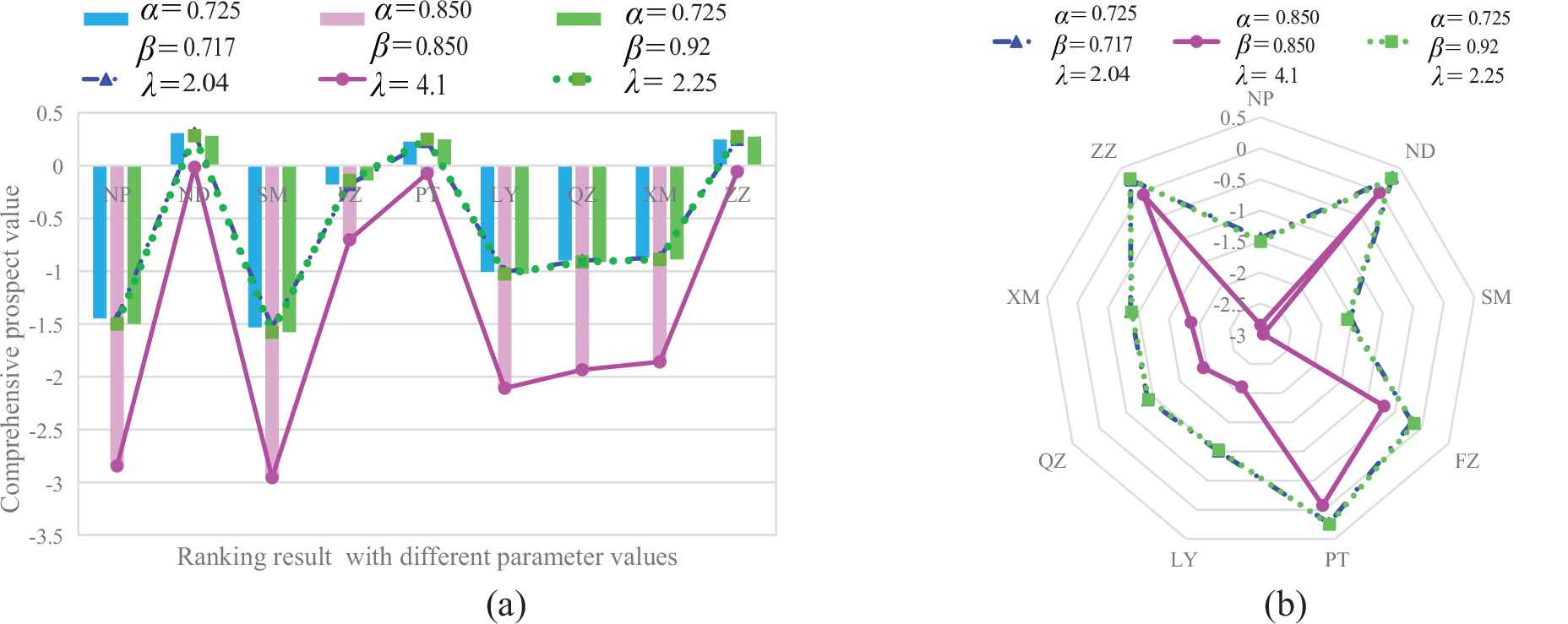
Ranking result with different parameter values α, β, and λ.
4.2.2. Comparative analysis with different methods
In order to illustrate the validity and rationality of the algorithm, the proposed method is compared with the most widely used operator-based method. Firstly, using the heterogeneous information conversion method [21], and the relationship between the TrFNN and other data, all kinds of heterogeneous data are converted into TrFNNs, and then the weighted comprehensive evaluation value of each city is calculated by using the trapezoidal fuzzy trapezoidal weighted arithmetic average operator (TNNWAA) [40]. Finally, the exact function and scoring function of the neutrosophic in trapezoidal fuzzy are used to rank the degree of city disaster. The TNNWAA operator is as follows:
The decision-making method steps based on the TNNWAA operator are as follows:
Step 1: By using the data conversion formula [21], the heterogeneous data of Table 3 is uniformly converted into the TrFNNs. The specific data are shown in Table 11:
| Index |
||||
|---|---|---|---|---|
| Cities | c1 | c2 | c3 | c4 |
| Nanping (NP) | ||||
| Ningde (ND) | ||||
| Sanming (SM) | ||||
| Fuzhou (FZ) | ||||
| Putian (PT) | ||||
| Longyan (LY) | ||||
| Quanzhou (QZ) | ||||
| Xiamen (XM) | ||||
| Zhangzhou (ZZ) |
| Index |
|||
|---|---|---|---|
| Cities | c5 | c6 | c7 |
| Nanping (NP) | |||
| Ningde (ND) | |||
| Sanming (SM) | |||
| Fuzhou (FZ) | |||
| Putian (PT) | |||
| Longyan (LY) | |||
| Quanzhou (QZ) | |||
| Xiamen (XM) | |||
| Zhangzhou (ZZ) |
Unified trapezoidal fuzzy neutrosophic numbers decision matrix
Step 2: Using the TNNWAA operator, the attribute values of each scheme are assembled to obtain a comprehensive evaluation value
Step 3: The comprehensive evaluation values are sorted according to different methods including Prospect Theory, TOPSIS and Traditional Function Method (also known as Score Function, Accuracy Function). The calculation results are shown in Table 12 and Figure 3.

City ranking results for different ranking methods.
| Index |
|||||||
|---|---|---|---|---|---|---|---|
| Cities | Prospect Theory |
TOPSIS |
Traditional Function Method |
||||
| Prospect Value | Ranking Results | Closeness Coefficients | Ranking Results | Score Function | Accuracy Function | Ranking Results | |
| Nanping (NP) | −1.921 | 8 | 0.0011 | 8 | 0.408 | −0.684 | 8 |
| Ningde (ND) | 0.895 | 1 | 1.0000 | 1 | 1.000 | 1.000 | 1 |
| Sanming (SM) | −2.004 | 9 | 0.0004 | 9 | 0.389 | −0.743 | 9 |
| Fuzhou (FZ) | 0.182 | 5 | 0.7965 | 5 | 0.748 | 0.328 | 5 |
| Putian (PT) | 0.496 | 4 | 0.9168 | 4 | 0.811 | 0.532 | 4 |
| Longyan (LY) | −1.277 | 7 | 0.0858 | 7 | 0.526 | −0.318 | 7 |
| Quanzhou (QZ) | −0.548 | 6 | 0.3834 | 6 | 0.632 | −0.013 | 6 |
| Xiamen (XM) | 0.895 | 1 | 1.0000 | 1 | 1.000 | 1.000 | 1 |
| Zhangzhou (ZZ) | 0.583 | 3 | 0.9498 | 3 | 0.840 | 0.606 | 3 |
Ranking results of different methods.
Step 4: It is known from the previous step the three different ranking results are the same, and the ranking of disaster severity in nine cities is
From the comparison of the two typhoon disaster assessment methods, it can be seen that although the ranking results are not exactly the same, they are basically the same, and the special optimal scheme is the same. In addition, because the TNNWAA operator is sensitive to data 0 when assembling information, the second method, which is based on the TNNWAA algorithm, sometimes cannot fully sort the evaluation objects. For example, the comprehensive evaluation values of ND and SM are the same, that is,
Compared with other related researches, the advantages of this algorithm mainly include several aspects:
The types of heterogeneous information studied in this paper are more comprehensive and more diverse, including ENs, interval numbers, language numbers, IFNs, IVIFNs, SVNNs, and TrFNNs. Compared with the literature [19], the heterogeneous data includes four types of data: real numbers, interval numbers, triangular fuzzy numbers, and IFNs. However, the information representation forms in our paper are more. Compared with the literature [20], the data type of our paper contains the NN and the TrFNN, while the literature [20] does not. Compared with the literature [21], the heterogeneous information includes real numbers, interval numbers, triangular fuzzy numbers, TrFNs, even so, the information representation forms in our paper are more. At the same time, compared with the literatures [22–25], the heterogeneous information in our paper research includes the NN and the TrFNN, however, the literatures [22–25] do not.
In this heterogeneous information environment, the attribute weight is determined based on the maximization of deviation. Compared with the subjective reference [76], the decision result of this paper is more objective and fair. Compared with the method [21], our method is easier to understand.
This paper adopts the PT to sort the selection is simple and easy to understand, and introduces the psychological behavior of the decision maker. Compared with the evidence reasoning [20], the calculation of our method is relatively small. Compared with the method [21] that transforms heterogeneous information into IvIFNs for information aggregation, our method can fully sort the evaluation objects without juxtaposed results.
5. CONCLUSION
Based on the study of heterogeneous information, this paper proposes a decision-making method based on PT and applies it to typhoon disaster assessment. The distance measures of heterogeneous data such as EN, interval number, linguistic number, IFN, IVIFN, NN, TrFNN, and so on are introduced. The attribute weighting of the heterogeneous information is determined by the deviation maximization method. Considering the uncertainty of typhoon disaster and the psychological perception of decision makers, the PT is used for disaster assessment. Finally, an example is given to verify the feasibility and effectiveness of the decision-making method, and the advantages of this method are compared with other methods. In the future work, the decision-making methods based on the NNs, the decision-making methods in the case of heterogeneous information incomplete situations, the study of compatibility and consistency of decision information, and their application in typhoon disaster assessment will be further studied.
CONFLICTS OF INTEREST
The authors declare no conflicts of interest.
AUTHORS' CONTRIBUTIONS
All authors have contributed to this paper. The individual responsibilities and contribution of all authors can be described as follows: The idea of this whole thesis was put forward by Ruipu Tan, she also wrote the paper. Wende Zhang analyzed the existing work of the research problem. Lehua Yang collected relevant data and implemented partial calculation through programming. The revision and submission of this paper was completed by Ruipu Tan and Shengqun Chen.
Funding Statement
The research was funded by [National Philosophy and Social Science Planning Office of China] grant number [17CGL058].
ACKNOWLEDGMENTS
This research is supported by the National Social Science Foundation of China (No. 17CGL058).
REFERENCES
Cite this article
TY  - JOUR
AU  - Ruipu Tan
AU  - Wende Zhang
AU  - Lehua Yang
AU  - Shengqun Chen
PY  - 2019
DA  - 2019/07/25
TI  - Multi-Attribute Decision-Making Method Based on Prospect Theory in Heterogeneous Information Environment and Its Application in Typhoon Disaster Assessment
JO  - International Journal of Computational Intelligence Systems
SP  - 881
EP  - 896
VL  - 12
IS  - 2
SN  - 1875-6883
UR  - https://doi.org/10.2991/ijcis.d.190722.002
DO  - 10.2991/ijcis.d.190722.002
ID  - Tan2019
ER  -