1. INTRODUCTION

In recent years, due to the rapid development of the network, our lives are closely related to the processing of images and videos. However, the traditional processing method usually has high sampling cost, redundant data, not only wasting time but also wasting a lot of hardware resources. It's urgently to solve these problems. In 2006, Candes et al. [19] mathematically proved that the original signal is reconstructed by the partial Fourier transform coefficient cocoa, which laid a theoretical foundation for compressed sensing (CS). Based on these results, Donoho [17] formally proposed the concept of CS and related theoretical frameworks. The theory says that as long as the signal is sparse itself or in a certain transform domain, a high-dimensional signal can be projected onto a low-dimensional space using an observation matrix that is not related to the sparse basis. Reconstructing sufficient information of the signal, so that the original signal can be reconstructed with high probability by solving optimization problems. The sampling rate is no longer determined by the signal bandwidth, but by the structure and content of the information in the signal.

The CS theory has been widely studied in the field of signal processing and has been paid more extensive attention [1–4,16,18]. CS theory carries out compression and sampling at the same time. Under certain conditions, the original signal can be recovered with high precision by collecting much smaller amount of information. Therefore, CS theory has brought a subversive breakthrough in information acquisition and processing technology. The theory of CS is simple, which greatly reduces the coding complexity. In addition, the CS eliminates the redundant information in the signal processing, and compresses the data while sampling, thereby saves much resource consumption. Therefore, CS is widely used. However, the performance of the traditional compression sensing reconstruction algorithm is not perfect. Because the image has high dimension (up to millions of pixels), therefore, the reconstruction of the traditional algorithm complexity is high, the number of iterations, large amount of calculation, some algorithms of reconstruction precision is high, but takes time for a long time, some algorithm reconstruction time is short, but the reconstruction accuracy is not high, therefore, the reconstruction of the traditional algorithms can't good balance to refactor accuracy and time both.

In order to solve the bottleneck of traditional reconstruction algorithms, reduce the computational complexity and improve the quality of reconstruction, many scholars proposed to use convolutional neural network (CNN) to replace the optimization process [5–8], so as to accelerate the reconstruction stage. In reference [5], a superimposed noise reduction automatic encoder (SDA) is used to recover signals from under-sampled measurements. ReconNet [7] and Deepinverse [6] introduce CNN into the reconstruction problem, and use random Gaussian measurement matrix to generate measurement values.

Although ReconNet is a typical algorithm that applies CNN to CS, it also has shortcomings. Its reconstruction precision is not high, the image edge is fuzzy. On the basis of ReconNet, this paper deepens the layers of full convolution network, designs deeper network structure, expands the scale of full convolution network, and replaces the convolution core with smaller convolution core, because the superposition of multiple small convolution kernels is better than the single use of large convolution kernels, which can reduce the number of parameters and reduce the computational complexity.

The specific contributions of this paper are as follows:

• (i) This paper proposes a new image compression sensor reconstruction network CombNet, which consists of a full connection layer and a full convolution network. Its performance is better than the existing network. For this network, when the measurement rate is less than 0.1, the signal-to-noise ratio is higher, the signal-to-noise ratio decreases more slowly and the robustness is stronger.

• (ii) Full connection layer generates fairly good preliminary reconstructed images with faster speed and lower computational cost. Full connection layer is very suitable for image reconstruction tasks with limited computing resources and network bandwidth. Full connection layer plays an initial role in image restoration.

• (iii) Full convolution network further improves the reconstructed quality of network, restores the pixel information of image, and achieves better visual effect.

The organizational structure of this paper is as follows: Section 2 introduce CNN and the related work of using CNN to solve CS reconstruction problem. Section 3 introduces the proposed total convolution measurement network CombNet. Section 4 presents the experimental results of this method and the comparison of experimental data. The conclusions of this paper are presented in Section 5.

2. RELATED WORK

2.1. Convolutional Neural Network

2.1.1. CNN structure

In recent years, the powerful feature learning ability and classification ability of CNNs have attracted extensive attention. A typical CNN consists primarily of the input layer, the convolutional layer, the pooled layer, the fully connected layer, and the output layer, as Fig. 1 shown.

Figure 1

Typical structure of convolutional neural networks.

The input of CNN is usually the original image. The layer i of the CNN is denoted by Hi. Then the generation process of can be expressed as:

(1)Hi=fHi−1⊗Wi+bi

Where Wi denotes the weight vector of the convolution kernel i, the operation symbol ⊗ denotes that the convolution kernel is convolved with the image of layer i−1 or the feature map, the output after convolution is added to the offset vector bi of layer i. Finally, the feature map Hi of the i layer is obtained by the nonlinear excitation function fx.

The pooling layer usually follows the convolutional layer and downsamples the feature map according to certain downsampling rules. There are two main functions of the pooling layer: (i) Dimension reduction of feature maps; (ii) Keeping the feature scale unchanged to a certain extent. After multiple convolutional and pooled layers are alternately transmitted, CNN relies on a fully connected network to classify the extracted features to obtain an input-based probability distribution Y, as shown in (2).

(2)Yi=PL=li|H0;W,b

Based on the above definition, the working principle of CNN can be divided into three parts: network model definition, network training, and network prediction.

2.1.2. Network model definition

The network model definition needs to design the network depth, the function of each layer of the network, and the hyperparameters in the network according to the amount of data of the specific application and the characteristics of the data itself: λ,η, and so on. The model of CNNs needs to study the following aspects: model depth, convolution step size, excitation function, selection of hyperparameters, etc.

2.1.3. Network training

The CNN trains the parameters in the network through the back propagation of the residuals, but the over-fitting in the training process greatly affects the convergence performance of the training. In the current research, some effective improvement methods have been proposed: the random initialization network parameters based on the Gaussian distribution [20], initialize with trained network parameters, and the parameters of different layers of the CNN are initialized independently of each other [21].

2.1.4. Network prediction

The prediction process of CNN is to output the feature map at each level by forward-conducting the input data, and finally use the fully connected network to output the conditional probability distribution based on the input data. Studies have shown that the CNN high-level features of forward conduction have strong discriminating ability and generalization ability.

2.2. ReconNet

ReconNet is a representative work of low-resolution mixed images measured by neural network reconstruction of random Gaussian matrix. The frame is shown in Fig. 2.

Figure 2

ReconNet network architecture.

It can be seen from the previous traditional algorithms that in order to reconstruct high-quality images with CS technology, the image needs to be segmented, which can achieve special processing of complex information blocks, and at the same time reduce the complexity of reconstruction and improve the accuracy of reconstruction. ReconNet is also using this idea, which divides a scene into non-overlapping blocks and reconstructs each block by feeding corresponding CS measurements to its network. The reconstructed blocks are appropriately arranged to form an intermediate reconstruction of the image, which is then input into an off-the-shelf noise remover to remove the block effect and obtain the final output image.

There are many papers extended by ReconNet [8,13–15]. In reference [8], in the measurement section, the input is subjected to block measurement to obtain a measurement value. In the recovery section, all measurements of an image are reconstructed simultaneously, which allows the image to be recovered from the measurement at the same time, rather than recovering from the scattered measurements. Document 13 combines a linear mapping network with a residual network algorithm, reconstructs the residual network, and compares the different residual networks. In reference [14], the image is restored by a full convolution measurement network. The first layer of this full convolution measurement network is the convolutional layer, which is used to obtain measurements. The second layer is the deconvolution layer for recovering low-resolution images from the measured data. The high-resolution image is then reconstructed by a residual block. In reference [15], the fully connected layer is first used as a measurement, and the full connection layer and ReconNet are combined to form an adaptive measurement network. The measurement rate is determined by the size of the network input and the output of the full connection layer.

3. COMBNET

3.1. The CombNet Model

The algorithm in this paper compresses an image into an M dimensional vector as the input to the CNN, denoted as ΦX. Φ is an M×N dimensional observation matrix of size, M is measurement data, and X is a vectorized input image block. The flow chart is shown in Fig. 3. In this paper, N = 1024, Because this article is to reconstruct the image after dividing the image into 32 × 32 blocks. If smaller blocks are used, the processing of the image is more delicate, but the reconstruction time is long. With larger blocks, only important information can be reconstructed and the details are slightly insufficient. In order to balance the two, this paper chooses blocks of 32 × 32 size, which can not only save the reconstruction time, but also get a higher reconstruction quality.

Figure 3

Flow chart of the algorithm.

The total convolutional network structure of this paper is shown in Fig. 4. Except that the first layer of the network is a fully connected layer, the rest are convolutional layers. In the first layer and the second layer of the convolutional layer, a 1 × 1 convolutional kernel is used, where in the first layer generates 128 feature maps, and the second layer generates 64 feature maps. The third to seventh layers all use a 3 × 3 convolutional kernel, in which the third layer generates 32 feature maps, and the fourth layer to the sixth layer all generate 16 feature maps. The seventh layer generates 64 feature maps, and the second and ninth layers all use a 9 × 9 convolutional kernel to generate 32 feature maps. The tenth layer uses a 1 × 1 convolutional kernel to generate 16 maps. The feature map, the eleventh layer uses a 1 × 1 convolutional kernel, and generates a feature map. In the last layer, a 5 × 5 convolutional kernel is used to generate a feature map as the output of the network. The algorithm in this paper keeps the size of the feature map unchanged in all layers. Therefore, except for the first layer, the second layer, and the eleventh layer, the other layers need to be zero-padded. Common incentive layer functions are sigmoid, tanh, ReLU, Leaky ReLU, ELU, Maxout, this paper uses ReLU to reduce the computational complexity of the network and the training speed is also faster. The BM3D filter is used in this algorithm to remove the block effect caused by the quantization error after block quantization, because it balances the time complexity and reconstruction quality well.

Figure 4

Overview of the algorithm in this paper.

3.2. Training Network

This paper first constructs a measurement matrix Φ, randomly generates a Gaussian matrix of appropriate size, and then orthogonalize its rows. The measurement data set of the CS is obtained according to y=ΦX, and the CNN is trained with the measurement data, the trained input tag pair can be expressed as ΦX;X. The algorithm trains the network at four different measurement rates MR = 0.25, 0.10, 0.04, and 0.01. Because the total number of pixels per block is N = 1024, the number of measurements is n = 256, 100, 40, and 10.

As shown in Fig. 5, the 481 × 321 images are reconstructed by the sampling rate of 0.25, 0.10, and 0.04, and give the reconstructed images obtained by each. It can be found that the algorithm of this paper effectively processes the image texture details and significantly improves the image processing quality.

Figure 5

Effect diagram of reconstruction at different measurement rates (the pictures are taken from Berkeley image). It is well known that the lower the sampling rate, the less key information contained in the image and the greater distortion of the image. In this figure, at 10% measuring speed, you can clearly see the tiny fluff on the stem of the fifth pictures. At 4% of the measurement rate, the starfish Mantis, flower, and leaf can be clearly seen, and we can see their details intuitively. It satisfies the visual experience people need.

The training of the reconstructed network is based on 91 image sets [22]. The blocks of size 32 × 32 are uniformly extracted from these image sets, the stride is 14, and 21760 patches are obtained. These form the labels of the training set. The input to the training set is the corresponding CS measurement of the patch. Experiments show that this training set is sufficient to train deep networks.

All training is based on the Caffe platform [9,10]. The computer used in this article is Nvidia GEFORCE GTX 1060 3GB and the training lasted for three days. The loss function is the average reconstruction error for all training image blocks. Here we choose MSE as the loss function because we want to minimize the loss function and favors a high peak signal-to-noise ratio (PSNR). MSE is the square of the difference between the true value and the predicted value and then the summed average. It is easy to derive by the form of square, so it is often used as a loss function for linear regression. Given a set of high-resolution images xi and their corresponding low-resolution images yi, the formula for MSE is y=1m∑imyi−xi2. Where m is the total number of image blocks in the training set, xi is the ith patch, yi is the network output of ith patch.

4. EXPERIMENT

To illustrate the superiority of the improved algorithm, we apply the algorithm of this paper to the two images of the two iterative CS image reconstruction algorithms TVAL3 [11], D-AMP [12], ReconNet [7], DR²-Net [13], and FCMN [14]. According to the experimental results, the performance of each algorithm is analyzed and compared.

This paper is at four different sampling rates: 0.25, 0.1, 0.04, and 0.01. In both noisy and noiseless, the reconstruction experiments of each image in Fig. 6 are performed by four different algorithms. The PSNR is also compared, and the algorithm with higher reconstruction quality is obtained. In order to simulate the noiseless block CS, firstly, the image is divided into 32 × 32 non-overlapping blocks, and then the CS measurement values of each block are calculated using the same random Gaussian measurement matrix as the training data for different sampling rates. This article uses the code provided by the respective author on the website. The parameters of these algorithms, including the number of iterations, are set to default values. Table 1 lists the PSNR values in dB for the intermediate reconstruction (expressed as not using BM3D) and the final denoised version (represented by using BM3D).

Figure 6

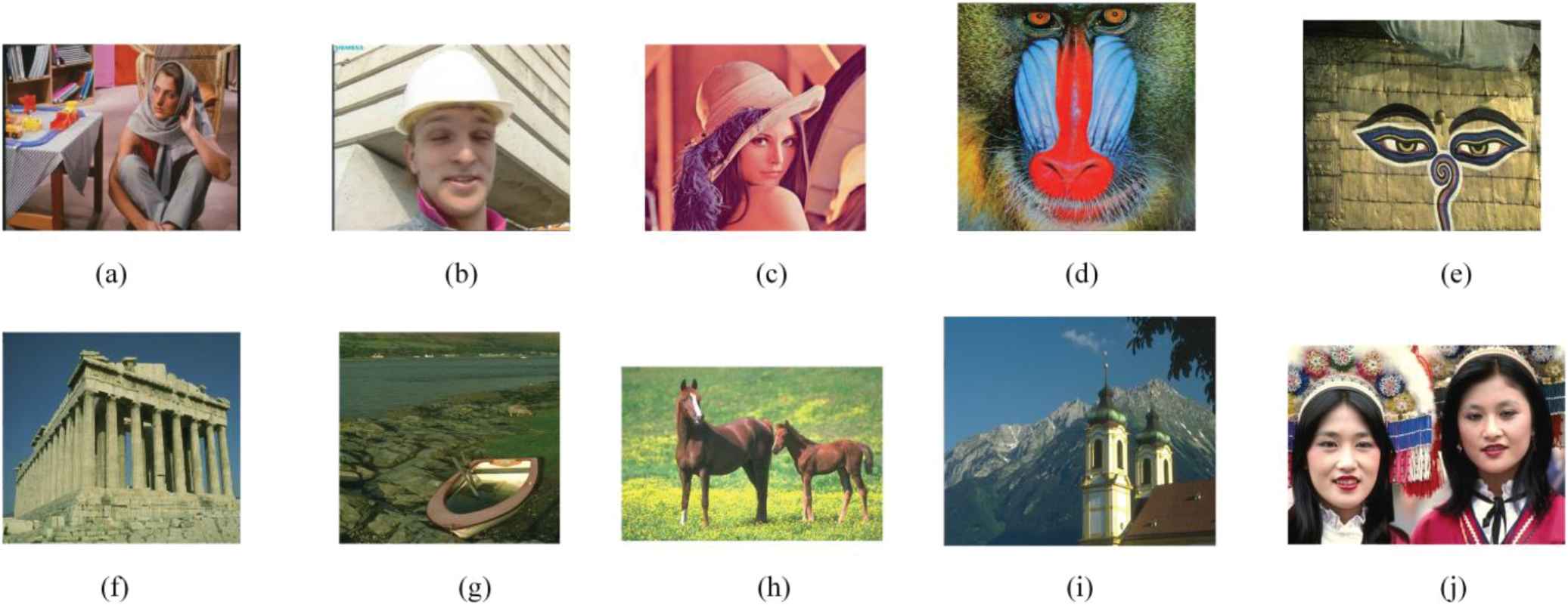
Six pictures to be compared: (a) barbara, (b) foreman, (c) lenna, (d) baboon, (e) 56028, (f) 67079, (g) 92059, (h) 113016, (i) 126007, (j) 189003. Among them, pictures starting from (e) are selected from Berkeley images.

According to the image processing method of the improved CS algorithm proposed in this paper, take the ten pictures in Fig. 6 as test images, and the simulation results are compared with the processing methods of TVAL3, D-AMP, ReconNet, DR²-Net, FCMN, and get the conclusion. The simulation data is shown in Tables 1 and 2 The subjective reconstruction quality of the images processed by the four algorithms is shown in Table 1. The average PSNR when using BM3D is shown in Table 2. Compared to the PSNR of images reconstructed by the other three algorithms, it can be seen that the PSNR of CombNet is significantly improved. An improvement in PSNR means that the smoothness will be better and the distortion will be reduced. By comparing the simulation data with the reconstruction quality, CombNet effectively improves the image processing quality, significantly reduces the loss of image detail, makes the reconstructed image clearer, and the reconstruction effect is better. In addition, CombNet's PSNR is higher when the sampling rate is low. Experiments have shown that CombNet can adapt to low sampling rate environments.

To verify the effect of different algorithms on reconstructed images at different sampling rates, we selected two images, as shown in Fig. 7. Among them, the first image has more detailed information, and more information needs to be reconstructed to reconstruct a high-quality images. The second picture is smoother, which does not require much reconstruction information to satisfy the visual experience. Therefore, this paper takes these two pictures as the representation of the reality image. Figure 7 shows the visual effect comparison of the original image, TVAL3, D-AMP, ReconNet, DR²-Net, FCMN, and the improved algorithm in this paper. The sampling rate of reconstruction is 0.1. It can be found that the reconstructed image of this algorithm is the closest to the original image, and the reconstructed image has the best effect.

Figure 7

Compare the reconstructed images of four different algorithms at a sampling rate of 0.1.

5. CONCLUSION

With the continuous development of image and video information processing, CS technology has been widely used in image processing. Since the CS technology only needs to collect a small amount of information, the original signal can be recovered and the coding complexity and resource consumption are reduced. Therefore, the CS technology is called a hotspot of image processing.

In the traditional theory of CS algorithms, the iterative algorithm has no advantage because of its algorithm and time complexity, as well as the effect of reconstruction. In order to adapt to the needs of image and video signal processing in today's social life, improve the speed and quality of image processing, and effectively solve the block effect in the process of block processing. This paper proposes a new network structure CombNet for CS image reconstruction. Simulation and verification prove that it provides excellent reconstruction quality when the sampling rate is high, retains rich image information, and can retain key image information when the sampling rate is low, which effectively improves the image processing quality.