International Journal of Computational Intelligence Systems

Volume 12, Issue 2, 2019, Pages 855 - 872

Matrix-Based Approaches for Updating Approximations in Multigranulation Rough Set While Adding and Deleting Attributes

Authors
Peiqiu Yu1, Jinjin Li1, *, Hongkun Wang2, Guoping Lin1
1School of Mathematics and Statistics, Minnan Normal University, Fujian, Zhangzhou, 363000, China
2Georgetown University, Washington, DC, 20057, USA
*Corresponding author. Email: jinjinlimnu@126.com
Corresponding Author
Jinjin Li
Received 18 January 2019, Accepted 20 June 2019, Available Online 5 July 2019.
DOI
10.2991/ijcis.d.190718.001How to use a DOI?
Keywords
Approximation computation; Multigranulation rough set; Knowledge acquisition; Decision-making
Abstract

With advanced technology in medicine and biology, data sets containing information could be huge and complex that sometimes are difficult to handle. Dynamic computing is an efficient approach to solve some problems. Since multigranulation rough sets were proposed, many algorithms have been designed for updating approximations in multigranulation rough sets, but they are not efficient enough in terms of computational time. The purpose of this study is to further reduce the computational time of updating approximations in multigranulation rough sets. First, searching regions in data sets for updating approximations in multigranulation rough sets are shrunk. Second, matrix-based approaches for updating approximations in multigranulation rough set are proposed. The incremental algorithms for updating approximations in multigranulation rough sets are then designed. Finally, the efficiency and validity of the designed algorithms are verified by experiments.

Copyright
© 2019 The Authors. Published by Atlantis Press SARL.
Open Access
This is an open access article distributed under the CC BY-NC 4.0 license (http://creativecommons.org/licenses/by-nc/4.0/).

1. INTRODUCTION

Since the rough set [1,2] was proposed by Pawlak in 1982, it has been widely used in various fields such as pattern recognition [310], machine learning [11,12], image processing [11,1319], decision-making [2022], data mining, and so on. A lot of extensions have been proposed to extend its application including covering based rough sets [23], variable precision rough sets [24], probabilistic rough sets [18], fuzzy rough sets [9,13,25,26], fuzzy variable precision rough sets [27], and so on.

Qian et al. proposed multigranulation rough sets (MGRSs) based on multiple equivalence relation in 2010, which include optimistic MGRSs and pessimistic MGRSs. In recent years, many models have been proposed based on two decision strategies: “Seeking common ground while reserving differences” and “Seeking common ground with eliminating differences.” For example, by popularizing the binary relation from equivalence relation to neighborhood relation, Lin et al. proposed neighborhood MGRSs. Lots of studies focus on deriving models by the same decision strategy. Huang et al. proposed intuitionistic fuzzy MGRSs [28]. Feng et al. proposed variable precision multigranulation decision-theoretic fuzzy rough sets [29]. Li et al. proposed three-way cognitive concept learning via multi-granularity [30]. There are research on MGRSs and their relative models, such as MGRSs theory over two universe [31], a comparative study of MGRSs and concept lattices via rule acquisition [32], and so on.

In an information explosion era, approximation computing becomes more and more difficult: the size of the data sometimes is too huge to handle, the structure of the data becomes more complex, and the granular structures often increase or decrease. The issue of computing and updating approximations in MGRSs and their derived models attracts much research interest. These studies are often categorized into four classes by scholars, namely, how to update approximations while varying attributes [33,34], how to update approximations while varying attribute values [35,36], how to update approximations while varying decision attribute values [33,37], and how to update approximations while varying object set [38,39].

No matter what variation is, there always exist two means to determine the relation between two sets: set operation or matrix product. By this viewpoint, we can classify those studies into two categories. One is based on set operation. Scholars use set operation to determine whether a set is contained in another set or not, or whether their intersection is empty or not (see Chuan Luo [20,21], Wenhao Shu [40], Guangming Lang [41], Mingjie Cai [42], Wei Wei [43], Xin Yang [44], etc.). When granules sizes are generally big, set operation is a time-consuming way because of its searching strategy: when we compute the intersection of two sets, we must confirm whether every object in a set is in another set or not. In the extreme case, when the two sets are both U (all samples are in one data set), then the time complexity of computing the intersection of them is |U|2. The other is based on matrix. These studies are mostly based on matrix product or other operations. Scholars often change a set into a binary matrix, and then design algorithms based on properties of binary matrix (see Jingqian Wang [45], Chengxiang Hu [46], Yanyong Huang [47] Yunge Jing [48], etc.). Although the time complexity of determining the relation between two sets via matrix approach is a constant, they often consider all the objects in the universe without filtering.

We attempt to combine the two approaches to derive new approaches to overcome their defect. In other words, we concentrate on which part of the universe does not need to be considered while computing and updating approximations in MGRS. At the same time, we determine the relation between two sets by matrix product. Why we try to propose the approaches? Because in real life application, it is common to add and delete attributes when there is some new information and some expired information. Different granular structures have a great influence on approximations in MGRS, thus different granular structures induce different decision-making processes. Moreover, adding and deleting attributes exists in the whole attribute reduction process. In decision-making and attribute reduction process, calculating approximations of decisions is an important and necessary step, so it is important to compute approximations based on approximations we have computed, that is, updating approximations. We need to proposed approaches for updating approximations because that updating approximations could be more efficient than compute the approximations again.

The purpose of this paper is to derive algorithms for updating approximations while adding and deleting attributes. First, searching region while updating approximations in MGRS need to be shrunk. A shrunk searching region can reduce the executing time of the algorithms. Second, matrix-based approaches for updating approximations need to be proposed to make algorithms more efficient.

The rest of this paper is organized as follows: Some basic concepts of rough set and MGRS are introduced in Section 2, and so is matrix-based static algorithm to calculate approximation in MGRS. In Section 3, dynamic approaches for updating approximations in MGRS while adding and deleting attributes are proposed. Several algorithms are proposed in Section 4. Experimental evaluations are conducted in Section 5 to verify the efficiency and validity of the algorithms that we designed. Finally, some conclusions and future work are given in Section 6.

2. PRELIMINARIES

In this section, we review some main concepts in MGRSs as well as static algorithm for computing approximations in MGRS.

2.1. Multigranulation Rough Sets

In the past few years, many extensions of MGRSs [49] have been proposed. Since MGRS are our basic model, we review the main results in this subsection.

Definition 1.

[1] Let IS=U,AT,VAT,f be an information system, where U=x1,x2,,xn is a nonempty finite set of objects called the universe. A=a1,a2,,ar is a nonempty finite set of attributes. The element AAT is called an attribute set. VAT=AATVA is a domain of attribute values, where VA is the domain of attribute set A. f:U×ATV is a decision function such that fx,AVA,AAT,xU.

Definition 2.

[49] Let IS=U,AT,VAT,f be an information system, where AkAT for any k1,2,,m. For any XU, the optimistic multigranulation lower and upper approximations of X are denoted by k=1mAkO_X and k=1mAkO¯X, respectively.

k=1mAkO_X=xU|xA1XxAmX.
k=1mAkO¯X=k=1mAkO_X,
where [x]Ak is the equivalence class of x in terms of the attribute set Ak, X is the complement of the set X.

Theorem 1.

[50] Let IS=U,AT,VAT,f be an information system, where AkAT for any k1,2,,m. For any XU, since [x]AkX, we have xX. The following result holds.

k=1mAkO_X=xX|xA1XxAmX.

Theorem 2.

[49] Let IS=U,AT,VAT,f be an information system, where AkAT for any k1,2,,m. For any XU, the optimistic multigranulation upper approximation of X is denoted by k=1mAkO¯X, we have

k=1mAkO¯X=xU|[x]A1XxU|[x]AmX.

Definition 3.

[49] Let IS=U,AT,VAT,f be an information system, where AkAT for any k1,2,,m. For any XU, the pessimistic multigranulation lower and upper approximation of X are denoted by k=1mAkP_X and k=1mAkP¯X, respectively.

k=1mAkP¯X=xU|xA1XxAmX.
k=1mAkP¯X=k=1mAkP_X.

Theorem 3.

[50] Let IS=U,AT,VAT,f be an information system, where AkAT for any k1,2,,m. For any XU, since [x]AkX, we have xX. The following result holds.

k=1mAkO_X=xX|xA1XxAmX.

Theorem 4.

[49] Let IS=U,AT,VAT,f be an information system, where AkAT for any k1,2,,m. For any XU, the optimistic multigranulation upper approximation of X is denoted by k=1mAkO¯(X), we have

k=1mAkP¯X=xU|xA1XxA2X[x]AmX.

2.2. Matrix-Based Algorithm for Computing Approximations in MGRSs

Definition 4.

[51] Let U=x1,x2,,xn. For any XU, the matrix representation of X is denoted by VX=v1X,,vnX, where

viX=1xiX0xiXi1,2,,n.

Lemma 5.

[52] Let U=x1,x2,,xn.X,YU, if YX, then

VYVtX=0,

“T” denotes the transpose operation, and “.” is matrix product.

Example 1.

Let IS=U,AT,VAT,f be an information system, as shown in Table 1, where U=x1,x2,x3,x4,x5,x6, B=Ad, and A=a1,a2,a3. Let X=x2,x4,x5. According to Definition 4, we have VX=0,1,0,1,1,0. Suppose Y=x2,x4, then VY=0,1,0,1,0,0. Obviously, YX. VX=1,0,1,0,0,1, VYVtX=0,1,0,1,0,01,0,1,0,0,1t=0.

U a1 a2 a3 d
x1 1 1 2 3
x2 2 3 3 3
x3 1 1 2 2
x4 2 2 3 2
x5 1 2 1 2
x6 1 1 1 3
Table 1

A decision information system.

Definition 5.

[53] Let IS=U,AT,VAT,f be an information system, where AkAT for any k1,2,,m. For any XU, the lower approximation character sets of X in MGRS can be calculated as

IAkLX=xAk|xAkXxX,k=1,2,,m.

Lemma 6.

[53] Let IS=U,AT,VAT,f be an information system, where AkAT for any k1,2,,m. For any XU, the pessimistic and optimistic lower approximations in MGRS can be calculated by

k=1mAkP_X=k=1mIAkUX,k=1mAkO_X=k=1mIAkUX.

Example 2.

(Continuation of Example 1) Suppose A1=a1, A2=a2,A3=a3, by Definition 5, we have

Vx2A1VtX=Vx4A1VtX=0,
Vx5A1VtX0,VIA1LX=0,1,0,1,0,0;
Vx2A2VtX=0,
Vx4A2VtX=Vx5A2VtX=0,
VIA2LX=0,1,0,1,1,0;
Vx2A3VtX=Vx4A3VtX=0,
Vx5A3VtX0,VIA3LX=0,1,0,1,0,0.

By Lemma 6,

Vk=1mAkP_X=k=1mVk=1mIAkLX
=VIA1LXVIA2LXVIA3LX=0,1,0,1,0,00,1,0,1,1,00,1,0,1,0,0=0,1,0,1,0,0.

By Definition 4,

k=1mAkP_X=x2,x4.
Vk=1mAkO_X=k=1mVIAkLX
=VIA1LXVIA2LXVIA3LX=0,1,0,1,0,00,1,0,1,1,00,1,0,1,0,0=0,1,0,1,0,0.

By Definition 4, k=1mAkO_X=x2,x4,x5.

Definition 6.

[53] Let IS=U,AT,VAT,f be an information system, where AkAT for any k1,2,,m. For any XU, the upper approximation character sets of X in MGRS can be defined as

IAkUX=xAk|xX,k=1,2,,m.

Lemma 7.

[53] Let IS=U,AT,VAT,f be an information system, where AkAT for any k1,2,,m. For any XU, the pessimistic and optimistic upper approximations can be calculated by

k=1mAkO¯X=k=1mIAkUX,k=1mAkP¯X=k=1mIAkUX.

Example 3.

Continuation of Example 2. From Table 1, we have

V[x2]A1=V([x4])A1=[0,1,0,1,0,0],V[x5]A1=[1,0,1,0,1,1];V[x2]A2=[0,1,0,0,0,0],V[x4]A2=V([x5]A2)=[0,0,0,1,1,0];V[x2]A3=V([x4]A2)=[0,1,0,1,0,0],V[x5]A3=[0,0,0,0,1,1];

By Definition 6,

VIA1UX=Vx2A1Vx4A1Vx5A1=1,1,1,1,1,1,VIA2UX=Vx2A2Vx4A2Vx5A2=0,1,0,1,1,0,VIA3UX=Vx2A3Vx4A3Vx5A3=0,1,0,1,1,1.

By Lemma 7,

k=1mAkO¯X=Vk=1mIAkUX
=VIA1UXVIA2UXVIA3UX=1,1,1,1,1,10,1,0,1,1,00,1,0,1,1,1=0,1,0,1,1,0.

By Definition 4,

k=1mAkP¯X=x2,x3,x4.
Vk=1mAkP¯X=k=1mVIAkUX
=VIA1UXVIA2UXVIA3UX=1,1,1,1,1,10,1,0,1,1,00,1,0,1,1,1=1,1,1,1,1,1.

By Definition 4,

k=1mAkO¯X=U.

Algorithm 1 [53] is a matrix-based algorithm for computing approximations in MGRS. The total time complexity of the algorithm is Om|X||U|. Steps 3–6 are to calculate IAkL and IAkU k1,2,,m whose time complexity is Om|X||U|. Steps 17–22 are to compute the approximations of MGRS whose time complexity is Om|U|.

Algorithm 1: Matrix-based algorithm for computing approximations in MGRS

Require: (1) An information system IS=U,AT,VAT,f (2) A target concept XU(3) Equivalence classes xAk,xU,k1,2,,m.

Ensure: Approximations in MGRS.

1: n|U|

2: m|X|

3: for i=1n do

4: for k=1m do

5: for j=1n do

6: if viX=1VtXVxiAk=0 then viIAkL=1

7: end if

8: if viX=1vjxiAk=1 then vjIAkU=1

9: end if

10: end for

11: end for

12: end for

13: Vk=1mAkO¯XVIA1U

14: Vk=1mAkP¯XVIA1U

15: Vk=1mAkP_XVIA1L

16: Vk=1mAkP_XVIA1L

17: for k=2m do

18: Vk=1mAkO_XVk=1mAkO¯XVIAkL

19: Vk=1mAkO¯XVk=1mAkO¯XVIAkU

20: Vk=1mAkP_XVk=1mAkP_XVIAkL

21: Vk=1mAkP¯XVk=1mAkP¯XVIAkU

22: end for

23: Return k=1mAkO_X,k=1mAkO¯X, k=1mAkP_X and k=1mAkP¯X

3. MATRIX-BASED DYNAMIC APPROACHES FOR UPDATING APPROXIMATIONS IN MGRS WHILE ADDING AND DELETING ATTRIBUTES

3.1. Matrix-Based Dynamic Approaches for Updating Approximations While Adding Attributes

In this subsection, we present matrix-based dynamic approaches for updating approximations in MGRS, while adding attributes, let ISt=U,ATt,VATt,ft be an information system at time t, ISt+1=U,ATt+1,VATt+1,ft+1 be an information system at time t+1, and for all AktATtkm, exists Akt+1ATt+1, such that AktAkt+1 for any k1,2,,m. Also, for all xU, we denote equivalence class of x at time t by [x]Akt. Denote equivalence class of x at time t+1 by xAkt+1. Denote pessimistic lower and upper approximations of X by k=1mAkt+1_PX and k=1mAkt+1¯PX at time t+1, respectively. Denote pessimistic lower and upper approximations of X by k=1mAkt_OX and k=1mAkt¯OX at time t + 1, respectively. Denote optimistic lower and upper approximations of X by k=1mAkt+1_OX and k=1mAkt+1¯OX at time t, respectively. Denote optimistic lower and upper approximations of X by k=1mAkt+1_OX and k=1mAkt+1¯OX at time t+1, respectively.

Lemma 8.

[46] Let ISt=U,ATt,VATt,ft be an information system at time t, ISt+1=U,ATt+1,VATt+1,ft+1 be an information system at time t+1. For any XU, the following results hold:

  1. k=1mAkt_OXk=1mAkt+1_OX;

  2. k=1mAkt¯OXk=1mAkt+1¯OX.

Lemma 9.

[46] Let ISt=U,ATt,VATt,ft be an information system at time t, ISt+1=U,ATt+1,VATt+1,ft+1 be an information system at time t+1. For any XU, the following results hold:

  1. k=1mAkt_PXk=1mAkt+1_PX;

  2. k=1mAkt¯PXk=1mAkt+1¯PX

Lemmas 8 and 9 indicate the relations of lower and upper approximations in MGRS between time t and time t+1. However, Lemmas 8 and 9 are not clear enough for updating approximation in MGRS. The following theorem provides accurate approaches for updating approximations in MGRS from time t to t+1.

Theorem 10.

Let ISt=U,ATt,VATt,ft be an information system at time t, ISt+1=U,ATt+1,VATt+1,ft+1 be an information system at time t+1. For any XU, we have

  1. If Δk=1mAk_O(X)={Xxk=1mAkt¯O(x)k=1mAkt_O(X)x|k{1,2,,m}, xAkt+1Xxk=1mAkt¯PXk=1mAkt_PX, then k=1mAkt+1OX=k=1mAkt_OXΔk=1mAk_OX

  2. If Δk=1mAk¯OX=Xxk=1mAkt¯O(x)k=1mAkt_O(X)x|k1,2,,m, xAkt+1X=xk=1mAkt¯PXk=1mAkt_PX, then k=1mAkt+1¯OX=k=1mAkt¯OXΔk=1mAk¯OX

  3. If Δk=1mAk_PX=Xxk=1mAkt¯O(x)k=1mAkt_O(X)x|k1,2,,m, xAkt+1Xxk=1mAkt¯PXk=1mAkt_PX, then k=1mAkt+1_PX=k=1mAktPXΔk=1mAk_PX

  4. If Δk=1mAk¯PX=Xxk=1mAkt¯O(x)k=1mAkt_O(X)x|k1,2,,m, xAkt+1X=xk=1mAkt¯PXk=1mAkt_PX, then k=1mAkt+1¯PX=k=1mAkt¯PXΔk=1mAk¯PX.

Proof.

    • If xk=1mAkt_PX, xk=1mAkt_PXxAktX, since we have yxAkt,yAkt+1xAkt,xAktXxAkt+1Xxk=1mAkt+1_OX.

    • If xk=1mAkt¯PXk=1mAkt_PX, xAkt+1Xxk=1mAkt+1_PX.

    • If xUk=1mAkt+1¯PX, from Definition 2, xAktX, since we have yxAkt,yAkt+1xAktxAkt+1Xxk=1mAkt+1_PX.

    • From the above, we have k=1mAkt+1_OX=k=1mAkt_OXΔk=1mAk_OX.

    • If xk=1mAkt_PX, xk=1mAkt_PX k1,2,,m,xAktX, Since we have yxAkt,yAkt+1xAkt, then k1,2,,m,xAktXk1,2,,m,xAkt+1Xx k=1mAkt+1_PXk=1mAkt+1¯OX, thus we have xk=1mAkt_PXxk=1mAkt+1¯OX.

    • If xk=1mAkt¯PXk=1mAkt_PX, k1,2,,m, xAkt+1X=xk=1mAkt+1¯OX.

    • If xUk=1mAkt¯PX, from Theorem 2, xUk=1mAkt+1¯PXk1,2,,m,xAktX=. Since yxAkt,k1,2,,m,yAkt+1xAkt, xAktX=xk=1mAkt+1¯PX.

    • From the above, we have k=1mAkt+1¯OX=k=1mAkt¯OXΔk=1mAk¯OX.

  1. It is similar to i.

  2. It is similar to ii.

Example 4.

(Continuation of Example 1) Suppose A1t=a1, A2t=a2; A1t+1=a1,a3, A2t+1=a2,a3, X=x2,x3,x4, thus we have

x1A1t=x3A1t=x5A1t=x6A1t=x1,x3,x5,x6,x2A1t=x4A1t=x2,x4x1A1t+1=x3A1t+1=x1,x3,x2A1t+1=x4A1t+1=x2,x4,x5A1t+1=x6A1t+1=x5,x6.
x1A2t=x3A2t=x6A2t=x1,x3,x6,x2A2t=x2;x4A2t=x5A2t=x4,x5;x1A2t+1=x3A2t+1=x1,x3,x2A2t+1=x2,x4A2t+1=x4,x5A2t+1=x5,x6A2t+1=x6.

From Definitions 2 and 3 we have

k=12Akt_OX=x2,x4,k=12Akt¯OX=U.
k=12Akt_PX=x2,k=12Akt¯PX=U.

By Theorem 10, we have

k=12Akt¯PXk=12Akt_PX=x1,x3,x4,x5,x6.

Since

x1A1t+1X,x3A1t+1X,x4A1t+1X,
x5A1t+1X,x6A1t+1X;
x1A2t+1X,x3A2t+1X,x4A2t+1X,
x5A2t+1X,x6A2t+1X.
x1A1t+1X,x3A1t+1X,x4A1t+1X,
x5A1t+1X=,x6A1t+1X=;
x1A2t+1X,x3A2t+1X,x4A2t+1X,
x5A2t+1X=,x6A2t+1X=.

Thus we have

k=12Akt+1_OX=k=12Akt_OXx4=x2,x4;k=12Akt+1¯OX=k=12Akt¯OXx5,x6=x1,x2,x3,x4.k=12Akt+1_OX=k=12Akt_PXx4=x2,x4,k=12Akt+1¯PX=k=12Akt¯PXx5,x6=x1,x2,x3,x4.

Definition 7.

Let ISt=U,ATt,VATt,ft be an information system at time t, ISt+1=U,ATt+1,VATt+1,ft+1 be an information system at time t+1. For any XU, the dynamic lower approximation character sets of X in MGRS while adding attributes can be defined as

ΔIAkL(X)={xk=12Akt¯P(X)k=12Akt_P(x)[x]Ak|[x]Akt+1Xxk=1mAkt¯P(X)k=1mAkt_P(X)},k=1,2,,m.

Definition 8.

Let ISt=U,ATt,VATt,ft be an information system at time t, ISt+1=U,ATt+1,VATt+1,ft+1 be an information system at time t+1. For any XU, the dynamic upper approximation character sets of X in MGRS while adding attributes can be defined as

ΔIAkU(X)={xk=12Akt¯P(X)k=12Akt_P(x)[x]Akt+1|[x]Akt+1X=xk=1mAkt¯P(X)k=1mAkt_P(X),k=1,2,,m.

Example 5.

(Continuation of Example 4)

ΔIA1L(X)={xk=12A2t¯P(x)k=12A1t_P(x)[x]A1|[x]A1t+1Xxk=12A2t¯P(X)k=12A1t_P(X)}={x4},
ΔIA2L(X)={xk=12Akt¯P(X)k=12Akt_P(x)[x]A2|[x]A2t+1Xxk=12A2t¯P(X)k=12A2t_P(X)}={x4};
ΔIA1U(X)={xk=12Akt¯P(x)k=1mAkt_P(x)[x]A1t+1|[x]A1t+1X=,xk=12Akt¯P(X)k=12Akt_P(X)}={x5,x6},
ΔIA2U(X)={xk=12Akt¯P(x)k=12Akt_P(x)[x]A2t+1|[x]A2t+1X=,xk=12Akt¯P(X)k=12Akt_P(X)}={x5,x6}.

Theorem 11.

Let ISt=U,ATt,VATt,ft be an information system at time t, ISt+1=U,ATt+1,VATt+1,ft+1 be an information system at time t+1. For any XU, we have

  1. Δk=1mAk_OX=ΔIAkLX|k=1,2,,m.

  2. Δk=1mAk¯OX=ΔIAkUX|k=1,2,,m.

  3. Δk=1mAk_PX=ΔIAkLX|k=1,2,,m.

  4. Δk=1mAk¯PX=ΔIAkUX|k=1,2,,m.

Proof.

This theorem can be easily obtained by Theorem 10 and Definitions 7 and 8.

By Theorem 11 we can easily obtain a matrix-based approach for updating approximations in MGRS while adding attributes.

Corollary 12.

Let ISt=U,ATt,VATt,ft be an information system at time t, ISt+1=U,ATt+1,VATt+1,ft+1 be an information system at time t+1. For any XU, we have

  1. Vk=1mAkt+1_OX=Vk=1mAkt_OXk=1mVΔIAkLX,

  2. Vk=1mAkt+1¯OX=Vk=1mAkt¯OXk=1mVΔIAkUX,

  3. Vk=1mAkt+1_PX=Vk=1mAkt_PXk=1mVΔIAkLX,

  4. Vk=1mAkt+1¯PX=Vk=1mAkt¯PXk=1mVΔIAkLX.

Proof.

This corollary is the matrix representation of Theorem 10.

Example 6.

(Continuation of Example 5)

  1. Vk=12Akt+1_OX=Vk=12Akt_OXk=12VΔIAkLX

    0,1,0,1,0,00,0,0,1,0,0=0,1,0,1,0,0,

  2. Vk=12Akt+1¯OX=Vk=12Akt¯OXk=12VΔIAkUX

    1,1,1,1,1,11,1,1,1,0,0=1,1,1,1,0,0,

  3. Vk=12Akt+1_PX=Vk=12Akt_PXk=12VΔIAkLX

    0,1,0,1,0,00,0,0,1,0,0=0,1,0,1,0,0,

  4. Vk=12Akt+1¯PX=Vk=12Akt¯PXk=12VΔIAkUX

    1,1,1,1,1,11,1,1,1,0,0=1,1,1,1,0,0.

From Definition 4 we have that k=12Akt+1_OX=x2,x4, k=12Akt+1¯OX=x1,x2,x3,x4; k=12Akt+1_PX=x2,x4, k=12Akt+1¯PX=x1,x2,x3,x4.

3.2. Matrix-Based Dynamic Approaches for Updating Approximations While Deleting Attributes

In this section, we present matrix-based dynamic approaches for updating approximations in MGRS, while deleting attributes, let ISt=U,ATt,VATt,ft be an information system at time t, ISt+1=U,ATt+1,VATt+1,ft+1 be an information system at time t+1, and for all AktATtkm, exists Akt+1ATt+1, such that Akt+1Akt for any k1,2,,m. Also, for all xU, we denote equivalence classof x at time t by xAkt. Denote equivalence class of x at time t+1 by xAkt+1. Denote pessimistic lower and upper approximations of X by k=1mAkt_PX and k=1mAkt¯PX at time t, respectively. Denote pessimistic lower and upper approximations of X by k=1mAkt+1_PX and k=1mAkt+1¯PX at time t+1, respectively. Denote optimistic lower and upper approximations of X by k=1mAkt_OX and k=1mAkt¯OX at time t, respectively. Denote optimistic lower and upper approximations of X by k=1mAkt+1_OX and k=1mAkt+1¯OX at time t+1, respectively. According to [46], we have the following results in this section:

Lemma 13.

[46] Let ISt=U,ATt,VATt,ft be an information system at time t, ISt+1=U,ATt+1,VATt+1,ft+1 be an information system at time t+1. For any XU, the following results hold:

  1. k=1mAkt+1_OXk=1mAkt_OX;

  2. k=1mAkt¯OXk=1mAkt+1¯OX.

Lemma 14.

[46] Let ISt=U,ATt,VATt,ft be an information system at time t, ISt+1=U,ATt+1,VATt+1,ft+1 be an information system at time t+1. For any XU, the following results hold:

  1. k=1mAkt+1_PXk=1mAkt_PX;

  2. k=1mAkt¯PXk=1mAkt+1¯PX.

Lemmas 13 and 14 indicate the relation of lower and upper approximations in MGRS between time t and time t+1. However, Lemmas 13 and 14 are not clear enough for updating approximation in MGRS. The following theorem provides accurate approaches for updating approximations in MGRS from time t to t+1:

Theorem 15.

Let ISt=U,ATt,VATt,ft be an information system at time t, ISt+1=U,ATt+1,VATt+1,ft+1 be an information system at time t+1. For any XU, we have

  1. If k=1mAk_O(X)={(Umk=1Akt¯O(x))x|k{1,2,,m}, xAkt+1Xxmk=1Akt_OXUmk=1Akt¯OX, then k=1mAkt+1_OX= mk=1Akt_OXmk=1Ak_OX.

  2. If k=1mAk¯O(X)={(Umk=1Akt¯O(X))x|k{1,2,,m}, xAkt+1Xxmk=1Akt_OX Umk=1Akt¯OX, then k=1mAkt+1¯OX= k=1mAkt¯OXk=1mAk¯OX.

  3. k=1mAk_P(X)={(Uk=1mAkt¯O(x))x|k{1,2,,m}, xAkt+1Xxmk=1Akt_OX Umk=1Akt¯OX, then k=1mAkt+1_PX= mk=1Akt_PXmk=1Ak_PX.

  4. If k=1mAk¯P(X)={(Utk=1Akt¯O(x))x|k{1,2,,m}, xAkt+1Xxmk=1Akt_OX Umk=1Akt¯OX, then k=1mAkt+1¯PX= mk=1Akt¯PXmk=1Ak¯PX.

Proof.

  1. By Lemma 13 we have k=1mAkt+1_OXk=1mAkt_OX, thus we have xk=1mAkt_OX,xAkt+1Xxk=1mAkt+1OX, in other words, xk=1mAkt_OX,xAkt+1Xxk=1mAkt+1_OX.

  2. By Lemma 13 we have k=1mAkt¯OXk=1mAkt+1_OX, thus we have k1,2,,m,xUk=1mAkt_OX, xAkt+1Xxk=1mAkt+1¯OX.

  3. It is similar to i.

  4. It is similar to ii.

Example 7.

(Continuation of Example 1) Suppose A1t=a1,a2,A2t=a2,a3; A1t+1=a2, A2t+1=a3, X=x2,x3,x4, thus we have

x1A1t=x3A1t=x6A1t=x1,x3,x6,x2A1t=x2,x4A1t=x4,x5A1t=x5;x1A1t+1=x3A1t+1=x6A1t+1=x1,x3,x6,x2A1t+1=x2.x4A1t+1=x5A1t+1=x4,x5.x1A2t=x3A2t=x1,x3,x2A2t=x2,x4A2t=x4,x5A2t=x5,x6A2t=x6;x1A2t+1=x3A2t+1=x1,x3,x2A2t+1=x4A2t+1=x2,x4;x5A2t+1=x6A2t+1=x5,x6.

From Definitions 2 and 3 we have

k=12Akt_OX=x2,x4,k=12Akt¯OX=x1,x2,x3,x4.
k=12Akt_PX=x2,k=12Akt¯PX=x1,x2,x3,x4,x6.

By Theorem 15, we have

k=12Akt_OXUk=12Akt¯OX=x2,x4,x5,x6.

Since

x2A1t+1X,[x4]A1t+1X,x5A1t+1X,x6A1t+1X.
x2A2t+1X,x4A2t+1X,x5A2t+1X,x6A2t+1X.
x2A1t+1X,x4A1t+1X,x5A1t+1X,
x6A1t+1X.
x2A2t+1X,x4A2t+1X,x5A2t+1X=,
x6A2t+1X=.

Thus we have

k=12Akt+1_OX=k=12Akt_OXx5,x6=x2,x4;k=12Akt+1¯OX=k=12Akt¯OXx2,x4=x1,x2,x3,x4.k=12Akt+1_PX=k=12Akt_PXx4,x5,x6=x2,k=12Akt+1¯PX=k=12Akt¯PXx2,x4,x5,x6=U.

Definition 9.

Let ISt=U,ATt,VATt,ft be an information system at time t, ISt+1=U,ATt+1,VATt+1,ft+1 be an information system at time t+1. For any XU, the dynamic upper approximation character sets of X in MGRS while deleting attributes can be defined as

IAkU(X)={(Uk=1mAkt¯O(x))[x]Akt+1|[x]Akt+1Xxk=1mAkt_O(X)(Uk=1mAkt¯O(X))},k=1,2,,m.

Definition 10.

Let ISt=U,ATt,VATt,ft be an information system at time t, ISt+1=U,ATt+1,VATt+1,ft+1 be an information system at time t+1. For any XU, the dynamic lower approximation character sets of X in MGRS while deleting attributes can be defined as

IAkU(X)={(Uk=1mAkt¯O(x))[x]Akt+1|[x]Akt+1Xxk=1mAkt_O(X)(Uk=1mAkt¯O(X))},k{1,2,,m}.

Example 8.

(Continuation of Example 7)

IA1L(X)={(Uk=1mAkt¯O(x))[x]A1|[x]A1t+1Xxk=1mAkt_O(X)(Uk=1mAkt¯O(X))}={x4,x5,x6}.
IA2LX=(Uk=1mAkt¯O(x))xA2|xA2t+1Xxk=1mAkt_OXUk=1mAkt¯OX=x5,x6.
IA1UX=(Uk=1mAkt¯O(x))xA1|xA1t+1X=xk=1mAkt_OXUk=1mAkt¯OX=x2,x4,x5,x6.
IA2UX=(Uk=1mAkt¯O(x))xA1|xA2t+1X=xk=1mAkt_OXUk=1mAkt¯OX=x2,x4.

Theorem 16.

Let ISt=U,ATt,VATt,ft be an information system at time t, ISt+1=U,ATt+1,VATt+1,ft+1 be an information system at time t+1. For any XU, we have

  • k=1mAkP_X=IAkLX|k=1,2,,m,

  • k=1mAk¯PX=IAkUX|k=1,2,,m,

  • k=1mAk_OX=IAkLX|k=1,2,,m,

  • k=1mAk¯OX=IAkUX|k=1,2,,m.

Proof.

This theorem can be easily obtained by Theorem 15 and Definitions 9 and 10.

By Theorem 16 we can easily obtain matrix-based approaches for updating approximations in MGRS while adding attributes.

Corollary 17.

Let ISt=U,ATt,VATt,ft be an information system at time t, ISt+1=U,ATt+1,VATt+1,ft+1 be an information system at time t+1. For any XU, we have

  • Vk=1mAkt+1_OX=Vk=1mAkt_OXk=1mVIAkLX,

  • Vk=1mAkt+1¯OX=Vk=1mAkt¯OXk=1mVIAkUX.

  • V(k=1mAkt+1P_(X))=V(k=1mAkt_P(X))(k=1mV(IAkL(X))),

  • Vk=1mAkt+1¯PX=Vk=1mAkt¯PXk=1mVIAkUX.

Proof.

This corollary is the matrix representation of Theorem 15.

Example 9.

(Continuation of Example 8)

  1. Vk=12Akt+1_OX=Vk=12Akt_OXk=12VIA2LX=0,1,0,1,0,01,1,1,1,0,0=0,1,0,1,0,0,

  2. Vk=12Akt+1¯OX=Vk=12Akt¯OXk=12VIAkUX=1,1,1,1,0,01,1,0,0,0,0=1,1,1,1,0,0.

  3. Vk=12Akt+1_PX=Vk=12Akt_PXk=12VIAkLX=0,1,0,0,0,01,1,1,0,0,0=0,1,0,0,0,0,

  4. Vk=12Akt+1¯PX=Vk=12Akt¯PXk=12VIAkUX=1,1,1,1,0,10,1,0,1,1,1=1,1,1,1,1,1.

From Definition 4 we have that k=12Akt+1_OX=x2,x4, k=12Akt+1¯OX=x1,x2,x3,x4, k=12Akt+1_PX=x2, k=12Akt+1¯PX=U.

Algorithm 2: Matrix-based algorithm for updating approximations in MGRS while adding attributes.

Require: (1) ISt=U,ATt,VATt,ft (2) ISt+1=U,ATt+1,VATt+1,ft+1 (3) A target concept XU (4) k=1mAkt_OX, k=1mAkt¯OX, k=1mAkt_PX and k=1mAkt¯PX. (4) Equivalence classes xAkt+1,xU,k1,2,,m.

Ensure: k=1mAkt+1_OX, k=1mAkt+1¯OX, k=1mAkt+1_PX, and k=1mAkt+1¯PX

1: n|U|

2: tk=1mAkt¯PXk=1mAkt_PX

3: for i=1t do

4: for k=1m do

5: if vik=1mAkt¯PXk=1mAkt_PX=1VXVtxiAkt+1=0 then viΔIAkL=1

6: end if

7: if vik=1mAkt¯PXk=1mAkt_PX=1VXVtxiAkt+1=0 then vjΔIAkU=1

8: end if

9: end for

10: end for

11: VΔk=1mAk_OXVΔIA1L

12: VΔk=1mAk¯OXVΔIA1U

13: VΔk=1mAk_PXVΔIA1L

14:VΔk=1mAk¯PXVΔIA1U

15: for k=2m do

16: VΔk=1mAk_OXVΔk=1mAk_OXVΔIAkL

17: VΔk=1mAk¯OXVΔk=1mAk¯OXVΔIAkU

18: VΔk=1mAk_PXVΔk=1mAk_PXVΔIAkL

19: VΔk=1mAk¯PXVΔk=1mAk¯PXVΔIAkU

20: end for

21:

22: Vk=1mAkt+1_OXVk=1mAkt_OXVΔk=1mAk_OX

23: Vk=1mAkt+1¯OXVk=1mAkt¯OXVΔk=1mAk¯OX

24: Vk=1mAkt+1_PXVk=1mAkt_PXVΔk=1mAk_PX

25: Vk=1mAkt+1¯PXVk=1mAkt¯PXVΔk=1mAk¯PX

26: Return k=1mAkt+1_OX,k=1mAkt+1_OX, k=1mAkt+1_PX and k=1mAkt+1¯PX

4. MATRIX-BASED DYNAMIC ALGORITHMS FOR UPDATING APPROXIMATIONS WHILE ADDING AND DELETING ATTRIBUTES

Based on Corollary 12, we propose matrix-based Algorithm 2 for updating approximations in MGRS while adding attributes. The total time complexity of Algorithm 2 is O(m|k=1mAkt¯P(X)k=1mAkt_P(X)||U|). Steps 3–12 are to calculate ΔIAkL and ΔIAkU k1,2,,m with time complexity O(m|k=1mAkt¯P(X)k=1mAkt_P(X)||U|). Steps 17–22 are to compute Δk=1mAk_OX,Δk=1mAk¯OX,Δk=1mAk_PX and Δk=1mAk¯PX with time complexity Om|U|. Steps 24–27 are to update the approximations of MGRS while increasing granular structures with time complexity O|U|.

Since the time complexity of Algorithm 1 is Om|X||U|, and in general, O(m|k=1mAkt¯P(X)k=1mAkt_P(X)||U|)O(m|X||U|) does not hold. Algorithm 3 is proposed to make sure the total time complexity is no more than Om|X||U|. In other words, when |k=1mAkt¯P(X)k=1mAkt_P(X)|>|X| we call Algorithm 1; otherwise, we call Algorithm 2.

Algorithm 3: Ensure total time complexity of updating approximations in MGRS while adding attributes is no more than O|X||U|.

Require: (1) ISt=U,ATt,VATt,ft (2) ISt+1=U,ATt+1,VATt+1,ft+1 (3) A target concept XU (4) k=1mAkt_OX, k=1mAkt¯OX, k=1mAkt_PX, and k=1mAkt¯PX. (4) Equivalence classes xAkt+1,xU,k1,2,,m.

Ensure: k=1mAkt+1_OX, k=1mAkt+1¯OX, k=1mAkt+1_PX and k=1mAkt+1¯PX

1: if |k=1mAkt¯PXk=1mAkt_PX||X| then Call Algorithm 2

2: end if

3: if |k=1mAkt¯PXk=1mAkt_PX|>|X| then Call Algorithm 1

4: end if

5: Return k=1mAkt+1_OX,k=1mAkt+1_OX, k=1mAkt+1_PX and k=1mAkt+1¯PX

Based on Corollary 17, we propose matrix-based Algorithm 4 for updating approximations in MGRS while deleting attributes. The total time complexity of Algorithm 4 is Om|k=1mAkt_OXUk=1mAkt¯OX||U|. Steps 3–12 are to calculate IAkL and IAkU k1,2,,m with time complexity Om|k=1mAkt_OXUk=1mAkt¯OX||U|. Steps 17–22 are to compute k=1mAk_OX, k=1mAk¯OX,k=1mAk_PX and k=1mAk¯PX with time complexity Om|U|. Steps 24–27 are to update the approximations of MGRS while increasing granular structures with time complexity Om|U|.

Algorithm 4: Matrix-based algorithm for updating approximations in MGRS while decreasing attributes

Require: (1) ISt=U,ATt,VATt,ft (2) ISt+1=U,ATt+1,VATt+1,ft+1 (3) A target concept XU (4) k=1mAkt_OX, k=1mAkt¯OX, k=1mAkt_PX and k=1mAkt¯PX. (4) Equivalence classes xAkt+1,xU,k1,2,,m.

Ensure: k=1mAkt+1_OX, k=1mAkt+1¯OX, k=1mAkt+1_PX and k=1mAkt+1¯PX

1: n|U|

2: tk=1mAkt_O(X)(Uk=1mAkt¯O(X))

3: for i=1t do

4: for k=1m do

5: if vik=1mAkt_OXUk=1mAkt¯OX=1VXVtxiAkt+1=0 then viIAkL=1

6: end if

7: if vik=1mAkt_OXUk=1mAkt¯OX=1viX=1 then viIAkU=1

8: end if

9: end for

10: end for

11: Vk=1mAk_OXVIA1L

12: Vk=1mAk¯OXVIA1U

13: Vk=1mAk_PXVIA1L

14: Vk=1mAk¯PXVIA1U

15: for k=2m do

16: Vk=1mAk_OXVk=1mAk_OXVIAkL

17: Vk=1mAk¯OXVk=1mAk¯OXVIAkU

18: Vk=1mAk_PXVk=1mAk_PXVIAkL

19: Vk=1mAk¯PXVk=1mAk¯PXVIAkU

20: end for

21:

22: Vk=1mAkt+1_OXVk=1mAkt_OXVk=1mAk_OX

23: Vk=1mAkt+1¯OXVk=1mAkt¯OXVk=1mAk¯OX

24: Vk=1mAkt+1_PXVk=1mAkt_PXVk=1mAk_PX

25: Vk=1mAkt+1¯PXVk=1mAkt¯PXVk=1mAk¯PX

26: Return k=1mAkt+1_OX,k=1mAkt+1_OX, k=1mAkt+1_PX and k=1mAkt+1¯PX

Since the time complexity of Algorithm 1 is Om|X||U|, and in general, Om|k=1mAkt_OXUk=1mAkt¯OX||U|Om|X||U| does not hold, Algorithm 5 is proposed to make sure the total time complexity is no more than Om|X||U|. In other words, when |k=1mAkt_OXUk=1mAkt¯OX|>|X| we call Algorithm 1; otherwise, we call Algorithm 4.

5. EXPERIMENTAL EVALUATIONS

In this section, several experiments were conducted to evaluate the effectiveness and the efficiency of Algorithm 3 (DMB) and Algorithm 5 (DMB). Three algorithms were chosen to compare, namely, matrix-based static algorithm (MB) [53], relation matrix-based static algorithm (RMB) [46], and relation matrix-based dynamic algorithm (DRMB) [46]. Six data sets were chosen from UCI machine learning repository. The details of the data sets are listed in Table 2. We can see that the sizes of data sets range from 194 to 1000, the attribute numbers range from 5 to 59. All the experiments were carried out on a personal computer with 64-bit windows 10, Inter(R) Core(TM) i7 6700HQ CPU @2.60 GHz, and 16GB memory. The program language was Matlab r2015b.

Algorithm 5: Ensure total time complexity of updating approximations in MGRS while deleting attributes is no more than O|X||U|

Require: (1) ISt=U,ATt,VATt,ft (2) ISt+1=U,ATt+1,VATt+1,ft+1 (3) A target concept XU (4) k=1mAkt_OX, k=1mAkt¯OX, k=1mAkt_PX and k=1mAkt¯PX. (4) Equivalence classes xAkt+1,xU,k1,2,,m.

Ensure: k=1mAkt+1_OX, k=1mAkt+1¯OX, k=1mAkt+1_PX and k=1mAkt+1¯PX

1: if |k=1mAkt_OXUk=1mAkt¯OX||X| then Call Algorithm 4

2: end if

3: if |k=1mAkt_OXUk=1mAkt¯OX|>|X| then Call Algorithm 1

4: end if

5: Return k=1mAkt+1_OX,k=1mAkt+1_OX, k=1mAkt+1_PX and k=1mAkt+1¯PX

No. Data Sets Samples Attributes
1 Blood Transfusion 748 5
2 Dermatology 366 20
3 Extention of ZAlizadehsani 303 59
4 Facebookmetrics 500 19
5 Flags 194 30
6 German Credit Data 1000 21
Table 2

Details of data sets.

5.1. Comparison of Computational Time Using Data Sets with Different Size

The computational time were compared among the four algorithms in MGRSs while adding and deleting attributes when the size of data sets increases. First of all, we construct three granular structures. We randomly chose an attribute set A^ containing at least two attributes in the data set and divided the rest into three parts randomly to contribute to three granular structures respectively. While adding attributes, we added the attributes in A^ into the three granular structures at the same time. While deleting attributes, we combined A^ with each granular structure and deleted the attributes in A^ from the granular structures at the same time. We randomly divided each data set U into 10 subsets U1,U2,,U10. Then U1 was chosen as the first temporary data set. After that, some samples of temporary data set were randomly selected to contribute to the target concept X. The size of target concept X wasabout 0.85 times the size of each temporary data set. We calculated the four approximations in MGRS by the four algorithms 10 times and compared the averages. Then made U1U2 the second temporary data set and repeat the whole process was repeated.

When the size of data sets increases, results of the four algorithms while adding and deleting attributes in MGRS are shown in Figures 1 and 2. We can see that DMB is the most efficient algorithm when the size of data set increases gradually. From Figure 1 we can see that DMB is effective and it reduces the computational time.

Figure 1

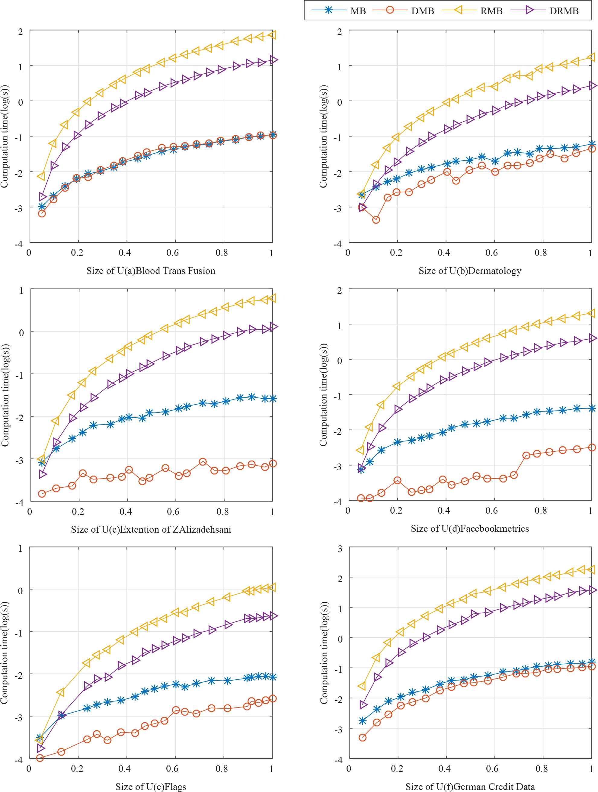
Computational time of Algorithm 3 when the size of U increasing gradually (adding attributes).

Figure 2

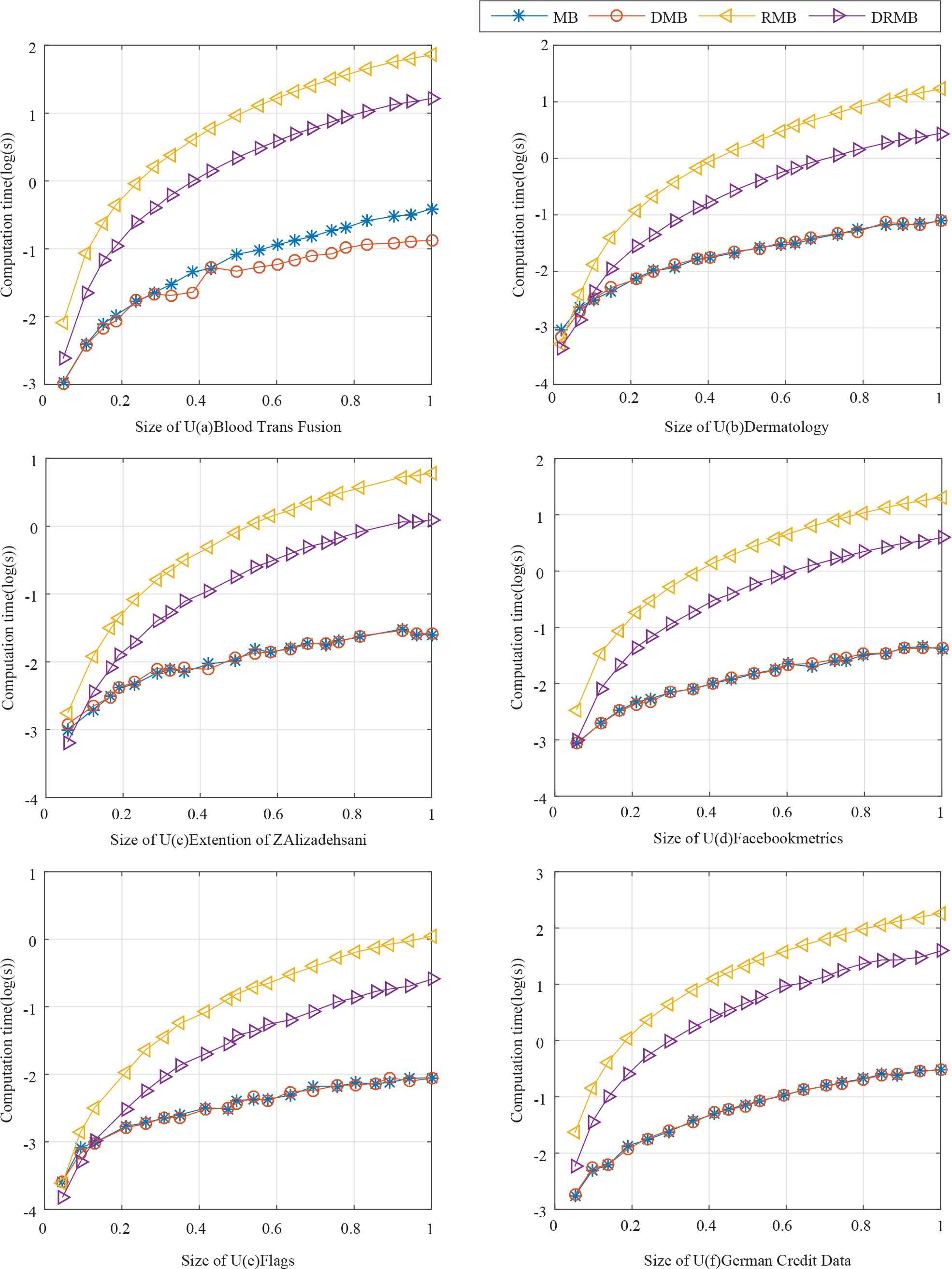
Computational time of Algorithm 5 when the size of U increasing gradually (deleting attributes).

5.2. Comparison of Computational Time Using Target Concept with Different Size

Similarly, instead of construct temporary data sets, we construct temporary target concepts. The process of constructing and varying the three granular structures is similar to Section 5.1. We randomly divided each data set into ten subsets X1,X2,,X10. And then X1 was chosen as the first temporary target concept. Finally, we calculated the four approximations in MGRS by the the four algorithms 10 times and compared the averages. Then made X1X2 the second temporary target concept and the whole process was repeated.

When the size of target concept increases, results of MB, DMB, RMB, DRMB are shown in Figures 3 and 4. When the size of target concept increasing gradually, RMB is always the most time-consuming algorithmn the four algorithms. DMB and MB are more efficient than RMB and DRMB. The computational time of DMB is always less than or equal to MB, so DMB is more efficient than any other algorithms. Sometimes the computational time of DMB is a little more than the MB while deleting attributes, which is due to additional computation in DMB and it is within the expected range.

Figure 3

Computational time of Algorithm 3 when the size of X increasing gradually (adding attributes).

Figure 4

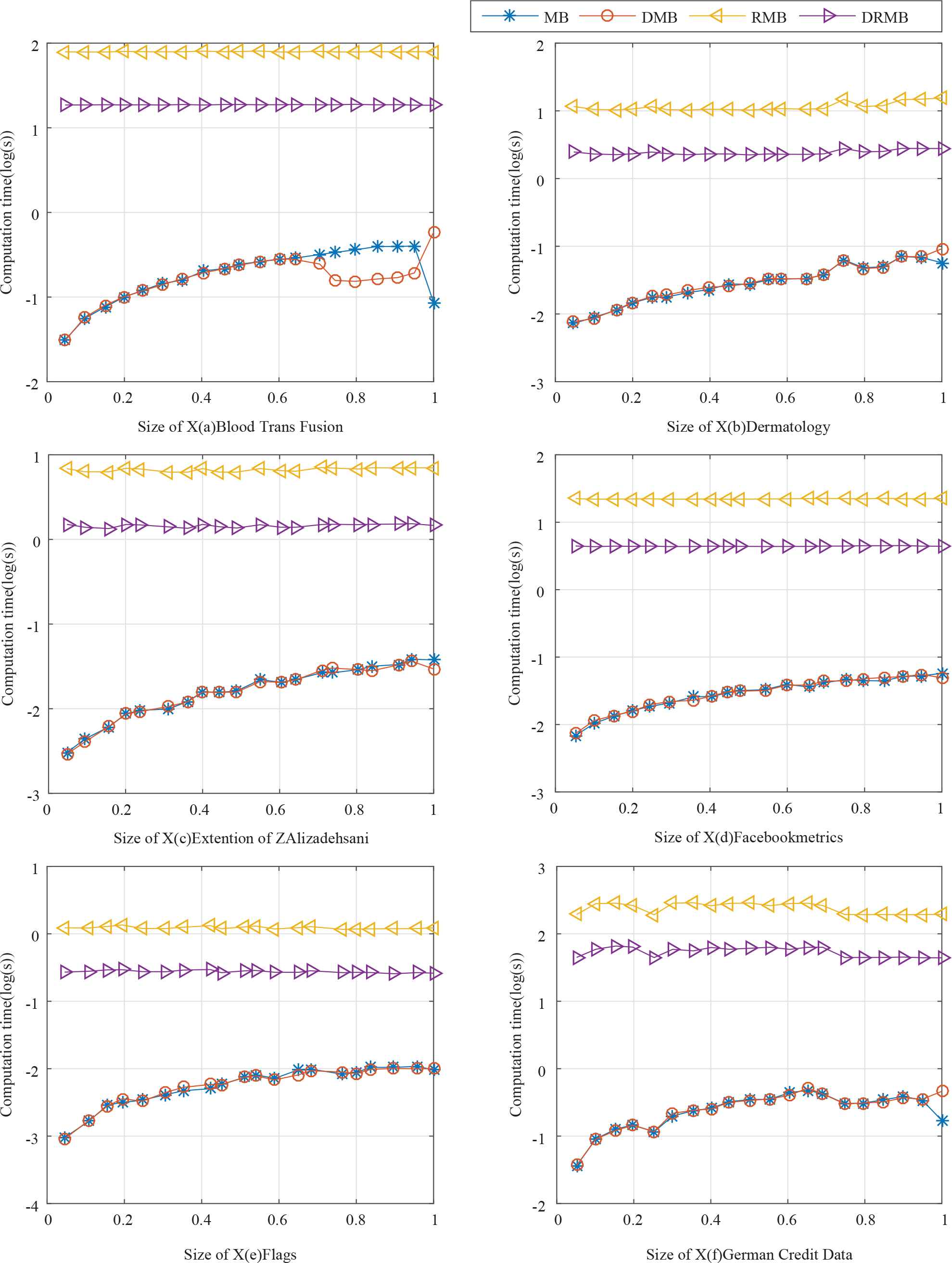
Computational time of Algorithm 5 when the size of X increasing gradually (deleting attributes).

6. CONCLUSION

Data sets in real life application sometimes are complex and huge, which is difficult to handle. In addition, the granular structures often increase and decrease in some data sets. It is important to design algorithms to update approximations in MGRS while adding and deleting attributes. In this paper, four algorithms have been proposed to ensure that the time complexity of the incremental algorithm is less than or equal to the static algorithm. Experimental results show that the computational time of the DMB is no more than the other algorithms in most of the situations.

Approximation computation is a basic process of attribute reduction. In the future, we will further investigate attribute reduction algorithm using the approaches we proposed.

CONFLICT OF INTEREST

There are no conflicts of interest.

AUTHORS' CONTRIBUTIONS

Jinjin Li and Peqiu Yu conceived and designed the study. Peiqiu Yu performed the experiments. Peiqiu Yu wrote the paper. Peiqiu Yu and Hongkun Wang reviewed and edited the manuscript. All authors read and approved the manuscript.

Funding Statement

This work is supported by National Natural Science Foundation of China (No.11871259), National Natural Science Foundation of China (No.61379021), National Youth Science Foundation of China (No.61603173), Fujian Natural Science Foundation of China (No.2019J01748).

ACKNOWLEDGEMENT

This work is supported by National Natural Science Foundation of China (No.11871259), National Natural Science Foundation of China (No.61379021), National Youth Science Foundation of China (No.61603173), Fujian Natural Science Foundation of China (No.2019J01748).

REFERENCES

42.M. Cai and G. Lang, Incremental approaches to updating attribute reducts when refining and coarsening coverings, 2018. arXiv Information Theory arXiv:1809.00606v1
52.Y. Cheng, Research on Covering Rough Set Algorithm Based on Matrix, AnHui Univercity, Hefei, Anhui, 2017. PhD thesis
Journal
International Journal of Computational Intelligence Systems
Volume-Issue
12 - 2
Pages
855 - 872
Publication Date
2019/07/05
ISSN (Online)
1875-6883
ISSN (Print)
1875-6891
DOI
10.2991/ijcis.d.190718.001How to use a DOI?
Copyright
© 2019 The Authors. Published by Atlantis Press SARL.
Open Access
This is an open access article distributed under the CC BY-NC 4.0 license (http://creativecommons.org/licenses/by-nc/4.0/).

Cite this article

TY  - JOUR
AU  - Peiqiu Yu
AU  - Jinjin Li
AU  - Hongkun Wang
AU  - Guoping Lin
PY  - 2019
DA  - 2019/07/05
TI  - Matrix-Based Approaches for Updating Approximations in Multigranulation Rough Set While Adding and Deleting Attributes
JO  - International Journal of Computational Intelligence Systems
SP  - 855
EP  - 872
VL  - 12
IS  - 2
SN  - 1875-6883
UR  - https://doi.org/10.2991/ijcis.d.190718.001
DO  - 10.2991/ijcis.d.190718.001
ID  - Yu2019
ER  -