1. INTRODUCTION

Demands for industrial process control are increasing with the flourishing development of modern industry [1]. Since process variables are often highly related to the quality of the final product, controlling these variables in a timely and precise manner is important. In a typical process, some variables are key indicators of process performance. However, most variables are difficult to measure due to several issues, including economic problems, environmental harshness, technical constraints, and severe time-delay. Soft sensor technology is often used to solve such problems [2,3]. Soft sensor technology allows accurate and real-time online measurement of variables dominant to a process, thereby rendering stable process control and ensuring the quality and economic benefits of industrial products. Thus, soft sensors are an important research field in modern control.

Soft sensor modeling methods are of three types, namely, first-principles models (FPMs), data-driven models, and mixed models (combination of FPMs with data-driven models). FPMs require prior knowledge of the mechanism of process objects and usually need to idealize and simplify some of the processes. Thus, implementation of FPMs to complex industrial processes is difficult. By contrast, data-driven models do not need detailed mechanistic information of the process during modeling as they only utilize the sample data from an industrial process to describe its state. Therefore, data-driven models are widely used in industrial processes [4]. A number of data-driven modeling methods are available, and these methods are mainly divided into two categories. One is based on multivariate statistical algorithms, including principal component regression (PCR) [5] and partial least-squares regression (PLS) [6], and the other is based on statistical machine learning algorithms, such as support vector regression (SVR) [7], genetic algorithm (GA) [8], and artificial neural network (ANN) [9]. Although these algorithms can be applied to various fields, some problems, such as those related to robustness and accuracy, still exist in the soft sensor modeling process. ANN has become an important modeling tool for soft sensors, but it only allows shallow learning, which presents a single hidden layer, and easily falls into a local optimum or undergoes gradient diffusion. Establishing an accurate and effective estimation model is a key endeavor in soft sensor modeling processes. Bengio et al. [10] proved that deep learning, a branch of machine learning, can overcome these complex problems well.

Deep learning, which was first proposed by Hinton and Salakhutdinov [11], is a data analysis and processing method. In recent years, it has received increased attention and gradually become a key research area of artificial intelligence [12]. Convolutional neural network (CNN), recurrent neural network (RNN), deep autoencoder (DAE), long short-term memory network, and deep belief network (DBN) are considered deep learning algorithms. Initially, deep learning was applied to the fields of image identification [13–16] and natural language processing [17–19]. Today, it is also gradually applied on process monitoring and modeling prediction [20–23]. Zhu et al. [24] issued a novel prediction method based on DBN that used linear regression as the final layer of its general structure. This model could examine the nonlinear and unstable features of internal valve leakage signals. Yan et al. [25] proposed a novel soft sensor modeling method that combines denoising autoencoders with a neural network (DAE-NN). In contrast to shallow learning methods, DAE-NN could remarkably improve the robustness and performance of predictions of the oxygen content in flue gasses in 1000 MW ultrasuperficial units. Despite their many benefits, however, these existing methods place all input variables into the network for training and barely consider the correlation between variables. Thus, even unimportant variables, which contribute to prediction errors, are treated equally when training the model.

Some works considering weighted features in deep neural networks have been reported. Yu and Yan [26] monitored and enhanced the layer-wise abnormal fluctuation information extracted by DBN to prevent this information from vanishing during the training process. The enhancement degree was determined by the fluctuation degree. The enhanced features showed the current working status by integrating support vector data, moving average filter, and kernel density estimation techniques, and the resulting method improved the detectability and performance of the Tennessee Eastman benchmark process. Yuan et al. [27] developed a soft sensor modeling with a variable-wise weighted stacked autoencoder (VW-SAE). This model considered the linear correlation between independent and dependent variables measured by the Pearson correlation coefficient before training. Application to estimations of butane content showed that this model achieves higher accuracy than three other methods. The method proposed by Yuan et al. [27] only calculated the linear correlation between independent and dependent variables. In fact, however, input and output variables are often highly nonlinearly correlated in the practical industrial process. The Pearson correlation coefficient cannot describe the nonlinear correlation between variables well. Although some variables are given relatively small weights, these variables and their effects on the output still exist during training. Furthermore, the number of variables collected at each sampling point may be massive during the industrial process, but not all input variables are useful or have a significant influence on the output variables due to differences in physical or chemical mechanisms. Thus, filtering redundant information while retaining unique feature information contained by other variables relevant to the output is particularly important.

Our work aims to uniformly select input variables and measure the relationships between them before training the network. We propose a novel SAE soft sensor modeling method based on maximal information coefficients (MICs) weighted between variable, hereinafter referred to as MICW-SAE. In this new model, the MIC between each input and output variables is initially calculated. If the MIC of one independent variable is lower than the threshold, the average MIC between this and the other variables is calculated. Whether this MIC must be changed to 0 is determined by comparing this average MIC and the second threshold. Thereafter, weights are proportionally assigned according to the adjusted MIC and added as a multiplier to the loss function of each autoencoder in SAE. The regression portion of this model is a simple ANN. Finally, the pre-training and fine-tuning processes are carried out as usual.

The rest of this study is organized as follows. First, a brief review of SAE and MIC is introduced in Section 2. Section 3 provides the detailed descriptions of our proposed method. Then, the Boston house-price dataset is used as a benchmark dataset to verify the effectiveness of our proposed method in Section 4. Following this step, our method is validated on the predicted output of naphtha dry points during the practical industrial process in Section 5. Finally, Section 6 draws our conclusions.

2. RELATED WORK

The concepts and basic algorithms of autoencoder (AE), SAE, and MIC are briefly reviewed in this section to introduce our proposed method in detail.

2.1. AE and SAE

AE, which was first proposed by Rumelhart in 1986, is a typical unsupervised machine learning method [28]. Hinton and Salakhutdinov [11] improved the structure of the original AE and introduced the concept of DAE. In DAE, the unsupervised layer-by-layer greedy training algorithm is first applied to complete the pre-training of the hidden layer. Then, the back-propagation (BP) algorithm is used to optimize the system parameters of the whole network, which can greatly improve the learning ability of the network and effectively solve the problem of local optimum observed in neural networks. This training mechanism has been widely used in deep learning.

In general, a three-layer neural network constitutes a common AE. In contrast to ANN, AE aims to reproduce input signals. Figure 1 shows the schematic structure of AE. The unlabeled sample dataset is assumed to be X=x1,x2,…,xn, where xi∈Rm. m denotes the number of variables and n is the number of samples. The input and hidden layers form the encoding portion to extract the features of input signals. The extracted feature is denoted as H=h1,h2,…,hn, where hi∈Rd and d indicates the number of nodes in the hidden layer. The encoding portion can be calculated as follows:

(1)h=s1W1x+b1,

where W1 and b1 denote the weight matrix and bias vector of the encoding process, respectively, and. s1⋅ is the activation function of the network. In this study, the sigmoid function, which is determined with below equation, is selected as the activation function of our model:

(2)ft=11+e−t.

Figure 1

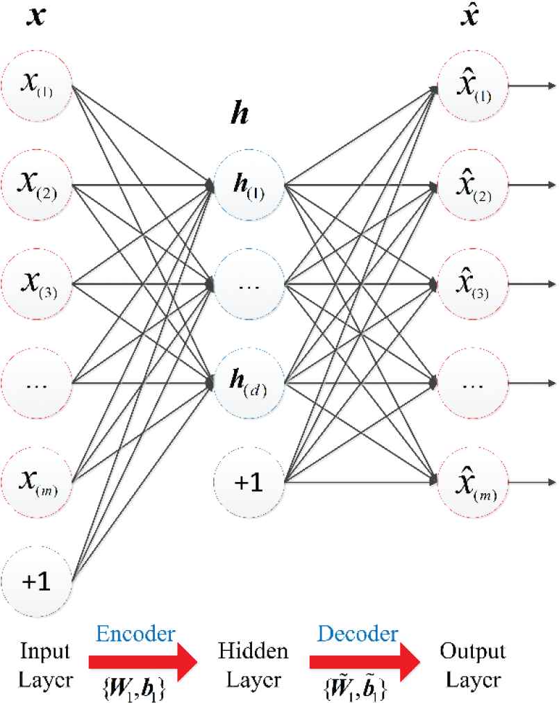
Schematic structure of autoencoder (AE).

The transformation process from the hidden layer to the output layer is called the decoding portion and used to reconstruct the input signal. The reconstructed signal can be expressed as X^=x^1,x^2,…,x^n, where x^i∈Rm. The decoding portion can be calculated as follows:

(3)x^=s2W~1h+b~1,

where W~1 and b~1 denote the weight matrix and bias vector of the decoding layer, respectively.

To make the input and output as equal as possible, AE uses the reconstructed error as a loss function, which can be described as:

(4)Lx,x^=12n∑i=1n∑j=1m‖xij−x^ij‖2.

SAE, which is an improved model of AE, was first developed by Bengio et al. [10] The training mechanism of SAE is divided into two steps: Layer-wise greedy unsupervised pre-training and supervised fine-tuning. First, SAE abandons the decoding portion of AE and only extracts the feature information obtained by AE. This feature information can represent the original information within the tolerance of the error, and, thus, the reconstructed process can be removed. Moreover, the extracted feature can be compressed once more by another AE. The AE in SAE is connected layer by layer. In other words, the feature achieved by the previous AE is the input signal of the next AE, which can be expressed as:

(5)hi=fθihi−1,2≤i≤ns,

where ns denotes the number of AEs in the whole network and fθi⋅ is the mapping function. The structure of SAE is shown in Figure 2. After pre-training, a multi-layer deep neural network with the same number of nodes as in the hidden layers in AEs is constructed. The weights and bias of each hidden layer Wi,bi are placed into the network as initial values, and the output of this network is set as labeled data and denoted as Y=y1,y2,…,yn, where yi∈Rk and k is the number of output variables. Afterwards, the BP algorithm is run to fine-tune the parameters of this network and minimize the error between the output of the model and the labeled data. Figure 3 illustrates the training procedure of fine-tuning.

Figure 2

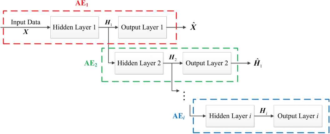
Structure of stacked autoencoder (SAE).

Figure 3

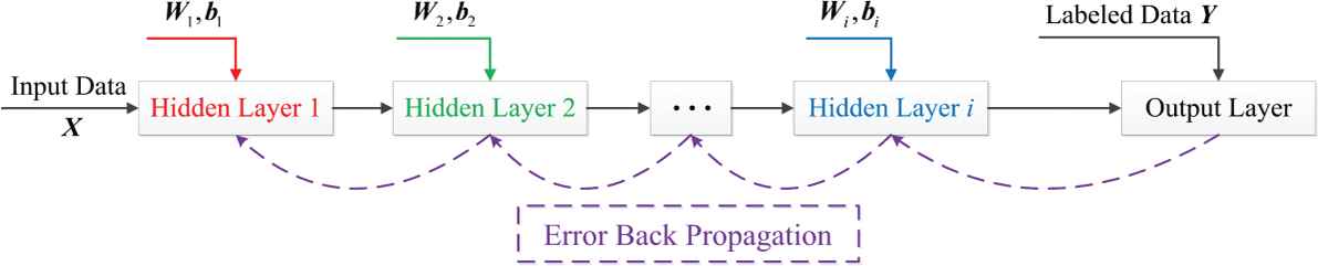
Training procedure of the fine-tuning.

3. METHODOLOGY

The layer-wise greedy pre-training and fine-tuning process can effectively solve the problems of neural networks easily falling into local optimum and gradient diffusion. Despite the powerful ability of SAE to extract the features of the original input data, irrelevant information in the output is still added to the network during the pre-training process if the input data are not judged by importance. In addition, the model developed by Yuan et al. [27] only considered the linear relationship between variables. In practical industrial processes, the mathematical relationship between variables is highly nonlinear and cannot be identified using Pearson or other traditional statistical correlation coefficients. MIC presents the advantage of describing both linear and nonlinear relationships. Simultaneously, although most independent variables have a strong mathematical functional relationship to the dependent variables, still there are some relatively minor independent variables that have a slight impact on the output signals. Those variables should be filtered to eliminate their impact on reducing the prediction accuracy.

As a result, we combined MIC with SAE to build a novel soft sensor modeling method. Assume the existence of a labeled dataset T=X,y, where X∈Rn×m, y∈Rn×1, n is the number of samples, and m expresses the number of measurable variables. Before pre-training, the MIC index, denoted as MICi between xi and y is first calculated, where i∈1,m. That is to say, the correlation between the ith independent variable and the labeled data is determined by the absolute value of MICi. Second, if MICi is greater than a relatively large threshold denoted as T1, then ith independent variable exerts a great influence on the dependent variable. Conversely, the sum of MICs between the ith input variable and each of the other input variables is obtained, and the average MIC is expressed as:

Finally, the weights are added to the loss function as a multiplier to train the network. Each AE in SAE will conduct this mechanism during pre-training and fine-tuning. The loss function is modified from Eq. (4) to:

Figure 4 presents the MICW-SAE structure. MICs naturally represent the correlation between the feature extracted from the previous AE and the labeled data since the second AE when pre-training, which means this mechanism of weighted MICs only targets the input signals of the current AE and the labeled data. By executing this step before pre-training, the primary variables directly affecting the output are gradually strengthened by the training progress due to the presence of large weights; secondary variables are gradually lost. Ultimately, the features abstracted by SAE for regression contain rich and valuable information representing the original input signal. Similarly, the variables must be weighted before fine-tuning.

Figure 4

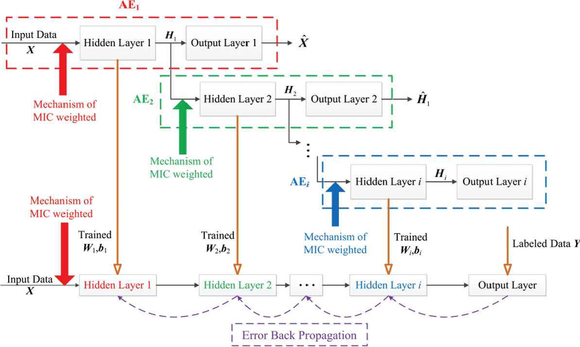
Structure of maximal information coefficient-stacked autoencoder (MICW-SAE).

To conclude, the MICW-SAE algorithm is conducted in a stepwise manner:

1. The thresholds are denoted as T1,T2, and i is set to 1.

2. The MIC of the ith independent and dependent variables is calculated and denoted as MICi.

3. If MICi>T1, then go to step (e); otherwise, the average MIC of the ith independent variable and other independent variables is calculated and denoted as avgMICi.

4. If avgMICi>T2, then MICi=0.

5. i=i+1. If i≤m, then go to step (b); otherwise, the weights of all variables are calculated according to Eq. (10).

6. The labeled dataset is normalized to 0,1. The standard dataset is divided into training TtrainXtrain,ytrain, valid Tvalid=Xvalid,yvalid, and test Ttest=Xtest,ytest datasets. Early stopping is applied to stop the training process on AE when the error of the valid dataset no longer decreases.

7. The aforementioned steps are carried out during layer-wise greedy pre-training and fine-tuning. Eq. (11) is used as the new loss function of all AEs in SAE and the whole fine-tuning network. Thereafter, the performance of soft sensor model is tested.

The flow chart in Figure 5 demonstrates our proposed modeling algorithm intuitively. The regression portion of MICW-SAE is a two-layer simple neural network. Two indicators, namely, the root mean squared error (RMSE) and the regression index R2, are applied to evaluate the model. The model with the lowest RMSE and the R2 closest to 1 is considered to provide the best effect on regression estimation. RMSE can be calculated as:

Figure 5

Flow chart of maximal information coefficient-stacked autoencoder (MICW-SAE).

4. EXPERIMENT AND RESULTS OF THE BOSTON HOUSE-PRICE DATASET

In this example, we take the Boston house-price dataset, which is available online in the sklearn library, as a benchmark dataset to verify the effectiveness of MICW-SAE. Benchmark data sets are generally used to illustrate the performance of the algorithm. The Boston house-price dataset contains 13 variables affecting the output, namely, average house-prices in Boston [31]. A total of 506 samples are included in this dataset. After random disruption, the numbers of training, valid, and test datasets are 323, 81, and 102, respectively.

The program is written in Python and run on a computer with an Intel Core i5-4590 (3.3 GHz) processor and 4 GB storage. MICW-SAE consists of three AEs, the hidden nodes of which number 7, 5, 3. The thresholds T1,T2 are set as 0.3 and 0.2 by trial-and-error method. Since the variables in the open machine learning database are all considerably relevant to the output, these two thresholds are relatively conservative. The weighted MIC mechanism forces the weight of one input variable to 0. The output of MICW-SAE is depicted in Figure 6, which shows that the predicted value of our model is very close to the true value. After the original input is enhanced and eliminated by weights calculated by MIC, nearly all sample points regress well to the true values. The number of sample points with large errors is also extremely small. This conclusion can be clearly drawn from Figure 7, which shows the absolute error of prediction by MICW-SAE. Despite the existence of one point with relatively great error, the predicted outputs of MICW-SAE on Boston house-price dataset are mostly fit well to their true values. Figure 8 proves whether the prediction error follows a Gaussian distribution. As shown in Figure 8, there are some error distribution intervals that do not strictly follow the red diagonal line indicates a normal distribution. However, most testing prediction errors lie roughly around the red diagonal line, which represents that our model prediction results basically match the local house-price pricing distribution. Thus, Figures 7 and 8 both verify the effectiveness and rationality of our proposed method.

Figure 6

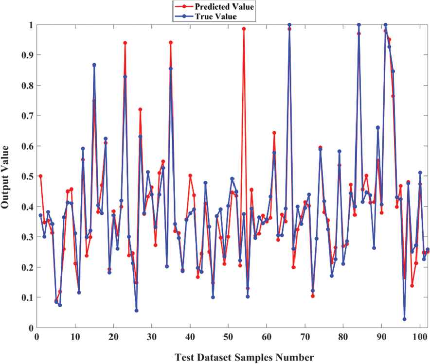
Results of estimation of the Boston house-price dataset by maximal information coefficient-stacked autoencoder (MICW-SAE).

Figure 7

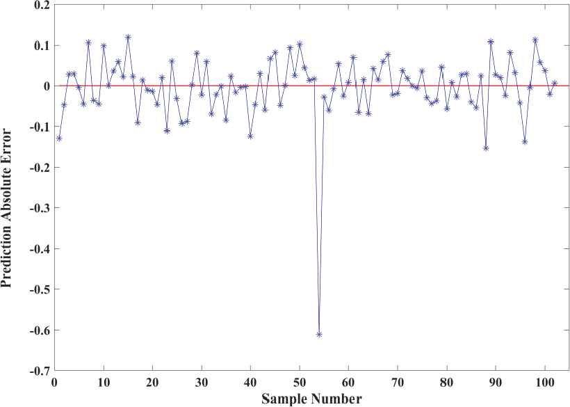
Plot of the prediction absolute errors by maximal information coefficient-stacked autoencoder (MICW-SAE) (Boston Dataset).

Figure 8

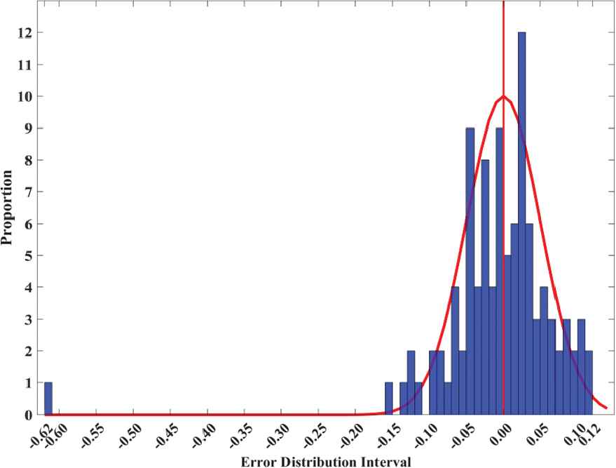
Histogram of the prediction absolute errors by maximal information coefficient-stacked autoencoder (MICW-SAE).

For comparison, four modeling methods based on machine learning, including partial least square (PLS), SVR, multi-layer ANN (M-ANN), and eXtreme Gradient Boosting (XGBoost) proposed by Chen and Guestrin [32] are applied to the same dataset. Moreover, three deep learning methods based on SAE (without weighted MICs), VW-SAE [27] as mentioned above and SAE-MIPCA-NN proposed by Wang and Yan [33] are also imported as comparative experiments. XGBoost, which is an extension of the Gradient Boosting Decision Tree (GDBT), has shown its good regression ability in various data mining competitions. The parameters are set as follows in this experiment: the max depth is 5, the learning rate is 0.1 and the number of trees is 20. SAE-MIPCA-NN uses principle component analysis (PCA) to extract the raw data and features weighted with MI above the threshold from each AE, and then regressed by ANN. The parameter setting method of this parallel experiment is the same as that of Wang and Yan [33]. As a result, the number of extracted components is eight. Additionally, because SVR does not require a valid dataset, the valid and training datasets are merged to train the SVR model in the experiments. The kernel function of SVR is the Gaussian radial basis function σ=1. The optimal component number chosen in PLS is 10 after 10-fold cross validation. The traditional SAE has the same hidden structure as MICW-SAE. The neuron numbers of M-ANN are also set to 13, 7, 5, 3, and 1. The same structures are also used in SAE, VW-SAE, and SAE-MIPCA-NN. The selection of batch size is consistent with that of MICW-SAE due to the random batch gradient descent algorithm in the neural network and AE on the computer. Table 1 shows the RMSE and R2 results of these comparative modeling methods and the best results are shown in bold. In comparison with the other models, MICW-SAE can predict housing prices in Boston more accurately with the lowest prediction error and the highest R2. These findings prove the effectiveness of our proposed method.

5. APPLICATION ON ATMOSPHERIC COLUMN

In this section, MICW-SAE is validated on a practical atmospheric column process. A description of this industrial process is first provided in Section 5.1. Next, an experiment to predict the naphtha dry point temperature is conducted, and seven regression modeling methods are used for comparison. Finally, an analysis and a discussion of the experiment results on the changing in the thresholds, the loss function value and reconstruction error are given.

5.1. Description of Atmospheric Column

Figure 9 shows a simple flow chart of an atmospheric column unit. The atmospheric column has 60 column plates. After heating by an atmospheric pressure kiln, the crude oil enters the fractionation distillation tower, and the top of the tower is driven into a cold reflux, which controls the temperature to approximately 120 °C. The temperature gradually increases from the top of the tower to the feeding section. Given different boiling point ranges, the gasoline vapor and steam are distilled from the top of the tower. Kerosene, light diesel oil, and heavy diesel oil are separately distilled from the No. 1, No. 2, and No. 3 side-streams, respectively [34]. The product at the top of the tower enters the reflux accumulator through the heat exchanger and condenser. Then, the product is pumped out by an atmospheric overhead pump. Part of the product is refluxed at the top of the tower, and another part is collected as the final product, naphtha. Naphtha is the distillate product obtained after the first step of crude oil distillation. The quality index of naphtha, as a raw material of the subsequent product, is an important consideration. However, the measurement accuracy of the naphtha dry point temperature is not ideal due to the large number of side-streams and complicated structure of the system, the diverse crude oil composition, and the high nonlinearity between variables. Thus, building a prediction model that can reliably estimate the naphtha dry point temperature and quality is essential. MICW-SAE is tested on this complex industrial process.

Figure 9

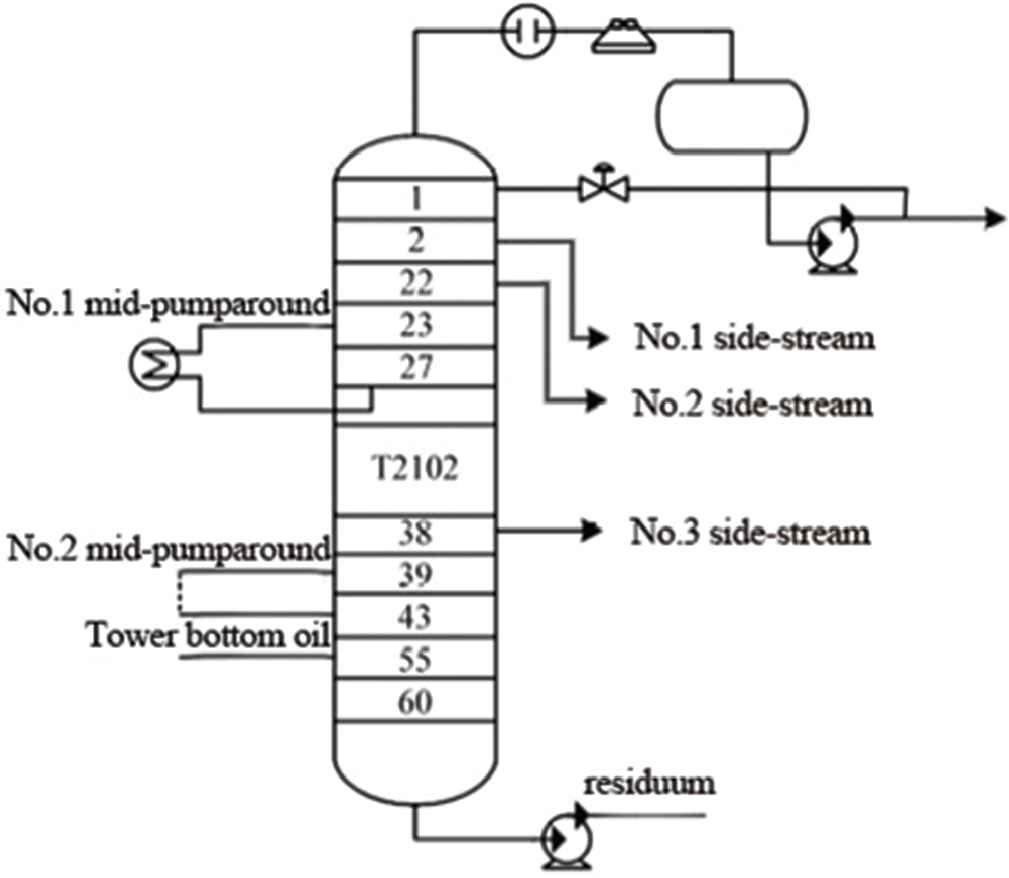
Flow chart of the atmospheric column.

5.2. Experiment on the Naphtha Dry Point Dataset

A total of 150 samples in the naphtha dry point dataset are collected from practical industrial processes. Table 2 provides a detailed description of each variable in this dataset. All samples are randomly disrupted, similar to the previous experiment. After normalization, the test dataset is composed of 30 samples; 120 samples are used as the training dataset, from which 24 samples are extracted as the valid dataset to monitor the training process. The batch size is set as 24 samples through the trial-and-error method. The thresholds T1,T2 are set as 0.2 and 0.26, respectively. Figure 10 shows that the MICs of input variables 3, 4, 7, 8, 9, 10, and 14 are below the threshold T1, which means these variables contain relatively less useful information than other variables. Figure 11 illustrates that, under the intervention of the threshold T2, the temperature and pressure at the top of the atmospheric column hardly affect the current dry point temperature and can be represented by other inputs. The final weights of all input variables are given in Table 3. The numbers of the three nodes in the hidden layer of AEs in SAE are 9, 6, and 4. Figure 12 gives the absolute error trend along with the test sample number in the naphtha dry point dataset by our proposed method. Since the dataset is acquired from the industrial processes, which contains large noises, most absolute errors of the prediction results are located between −0.1,0.1.

Figure 10

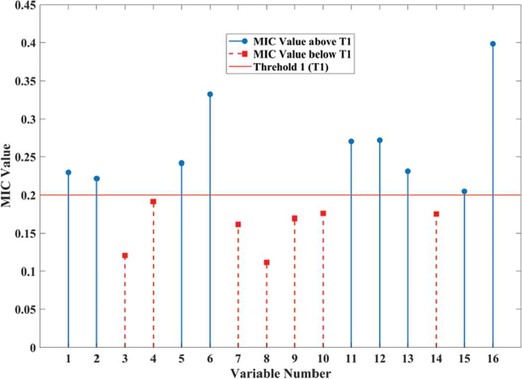
Maximal information coefficients (MICs) between input variables and output.

Figure 11

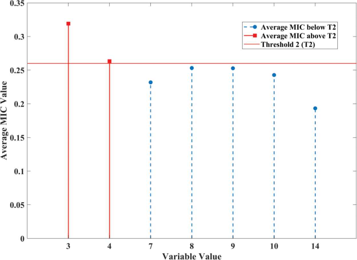
Average maximal information coefficients (MICs) of x_(i) below T₁.

No.	Variable Description
1	Total exit temperature
2	Total flow
3	Temperature at tower top
4	Pressure at tower top
5	Pumparound Energy at tower top
6	Product flow at tower top
7	Flow of light diesel oil
8	No.1 side-stream
9	No.2 side-stream
10	No.3 side-stream
11	Energy brought by circulation at top tower
12	Energy of No.1 mid-pumparound
13	Energy of No.2 mid-pumparound
14	Vaporization temperature
15	Stripping steam flow
16	Previous value of naphtha dry point

Table 2

Description of each variable in the naphtha dry point dataset.

Variable No.	Weight
x1	0.071943
x2	0.069409
x3	0
x4	0
x5	0.075694
x6	0.103963
x7	0.050637
x8	0.034854
x9	0.053006
x10	0.054964
x11	0.084609
x12	0.085078
x13	0.072433
x14	0.054684
x15	0.064075
x16	0.124650

Table 3

Weights of each variable in the naphtha dry point dataset.

Figure 12

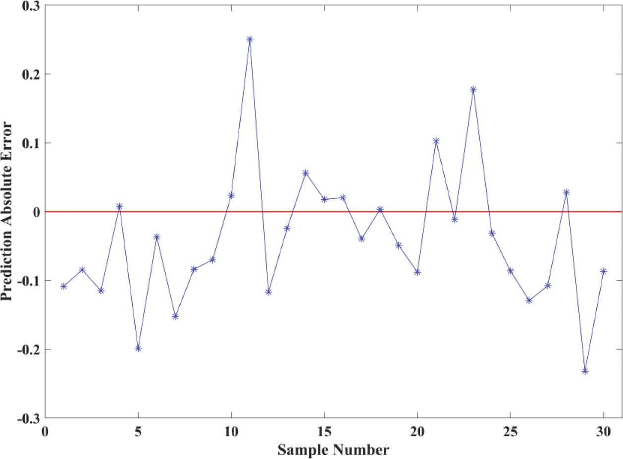
Plot of the prediction absolute errors by maximal information coefficient-stacked autoencoder (MICW-SAE) (Naphtha Dry Point Dataset).

The same training, valid, and test datasets are used with the seven other models, and the rules for setting the training dataset and parameters in these models are identical to those in the previous experiment. The radial basis function is still applied to SVR σ=0.1. The number of components is 7 in PLS. In XGBoost, the max depth is 4 and the number of trees is 30. The learning rate is set to 0.1, which the same as the previous experiment. The structures of SAE, VW-SAE, SAE-MIPCA-NN, and M-ANN are also consistent with MICW-SAE, and the batch size is 24 samples. In SAE-MIPCA-NN, nine eligible components are selected. The results of these models are provided in Table 4 and the optimal results are written in bold.

Model	RMSE	R2	MARE	Performance Increase (MARE)
MICW-SAE	0.161319	0.560128	0.043065	/
PLS	0.167904	0.490067	0.047862	10.02%
SVR	0.174369	0.466648	0.047105	8.58%
XGBoost	0.171400	0.491696	0.053284	19.18%
M-ANN	0.173193	0.217630	0.052893	18.58%
SAE	0.177296	0.451228	0.052668	18.23%
VW-SAE	0.165601	0.514201	0.045435	5.22%
SAE-MIPCA-NN	0.164790	0.523348	0.046048	6.48%

Table 4

RMSE, R2, and MARE results of the naphtha dry point test dataset.

5.4. Discussion

During the experiment process, the thresholds T1 and T2 are chosen by trial-and-error methods. To demonstrate the impact on the accuracy of MICW-SAE when these thresholds vary, we did a series of experiments shown in Tables 5 and 6. The last column in Tables 5 and 6 shows the number of variables will participate in the training under the mechanism we proposed. The best choices of T1 and T2 are written in bold. We find that different thresholds bring various effects on the final prediction accuracy of the model and the values shown in bold are also both optimal in their respective datasets. From Tables 5 and 6, we can conclude that when T2 remains unchanged, more input variables need to be further calculated and fewer variables are considered to contain the information directly related to the labeled data if T1 increases. In this case, only six and nine variables can be chosen to be trained as shown in Tables 5 and 6. The significant reduction in the number of input variables leads to a large loss of information when training so that the prediction effect becomes worse. Conversely, the metrics of mathematical relationship between the input and output variables becomes weak, which means that nearly all variables are considered useful and redundant information cannot be identified well in the case of a decrease in T1. Under this condition, all the input variables in the two datasets are involved in the training process. The prediction accuracy of the MICW-SAE is close to that of the VW-SAE compared Tables 1 and 4 with Tables 5 and 6. Notice that in the naphtha dry point dataset, when T1=0.1,T2=0.26, both VW-SAE and MICW-SAE use all input variables for training. However, the prediction effect of MICW-SAE is better than VW-SAE. This is mainly because MIC can measure the high nonlinearity relationship between variables more clearly than Pearson coefficient in industrial processes.

On the other hand, when T1 is unchanged, after all the input variables that has little relationship with the output are found, the increase of T2 enforces almost all the information contained in these selected variables considered to be unique. Thus, some variables that contain useless information are participated in the training resulting in a decrease in the prediction precision. On the contrary, when T2 is reduced, the information contained in the selected variable is always considered replaceable by other variables. Therefore, part of these minor variables, the information of which may be unique to the output, are also deleted. The elimination of these important information will also lead to a decline in prediction accuracy. Currently, there is no strong justification or index for these parameters setting. Trial-and-error method is the only feasible way to solve this problem at present. Consequently, how to find a suitable indicator to adjust the thresholds will be one of our research priorities in the future.

	RMSE	R2	Number of Train/Total Variables
T1=0.4,T2=0.2	0.115486	0.822850	6 / 13
T1=0.2,T2=0.2	0.095972	0.881375	13 / 13
T1=0.3,T2=0.2	0.083223	0.917145	12 / 13
T1=0.3,T2=0.3	0.096463	0.879099	13 / 13
T1=0.3,T2=0.1	0.088135	0.901740	11 / 13

Table 5

RMSE and R2 results of the Boston house-price dataset varies with T1 and T2.

	RMSE	R2	Number of Train/Total Variables
T1=0.3,T2=0.26	0.188237	0.442012	9 / 16
T1=0.1,T2=0.26	0.165230	0.517732	16 / 16
T1=0.2,T2=0.26	0.161319	0.560128	14 / 16
T1=0.2,T2=0.27	0.165026	0.528801	15 / 16
T1=0.2,T2=0.25	0.174754	0.455374	12 / 16

Table 6

RMSE and R2 results of the naphtha dry point dataset varies with T1 and T2.

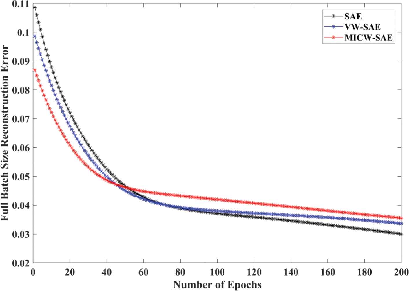
Furthermore, we investigated the reconstruction error of the different neural network models in the same batch size case. Figure 13 demonstrates the learning error of MICW-SAE, VW-SAE and SAE during fine-tuning within 200 epochs. SAE produces the highest learning errors among three methods surveyed at first because its loss function is without weights. Leading-in of the weighted process allows the variables in the VW-SAE and MICW-SAE models to be multiplied by 0,1 so that their loss functions decrease. We conducted another experiment to explain why the reconstruction error of SAE is lower than those of MICW-SAE and VW-SAE during later stage. The first AEs in both models are selected and trained to record their respective reconstruction errors and loss functions values. All parameters among the three models are identical. Table 7 illustrates that MICW-SAE has the second lowest loss function but the highest reconstruction error mainly because the weights obtained by MIC range from 0 to 1. Since the weights of the two independent variables are adjusted to 0 in MICW-SAE, the weights of the other variables are increased by contrast to VW-SAE, which contribute to a higher loss function value by MICW-SAE. When these weights are added to the loss function as multipliers, the loss function is bound to decrease and be lower than that of SAE. As for the larger reconstruction error, both the goal of MICW-SAE and VW-SAE network optimization are a new loss function multiplied by weights on the basis of the original reconstruction error. Compared with the loss function directly used in SAE as the optimization target, the reconstructed errors of MICW-SAE and VW-SAE are thus slightly higher. However, in the test and prediction process, the reconstruction error is pointless. The trained features and weights of hidden layers by AEs are actually used, and the prediction error is more concerned. Taken together, the test results of the two datasets prove the superiority of MICW-SAE over other modeling algorithms.

Figure 13

Loss function values of the three models.

	SAE	VW-SAE	MICW-SAE
Loss function value	0.004084	0.000171	0.000194
Reconstruction error	0.004084	0.004865	0.010889

Table 7

Reconstruction errors of the first AE in MICW-SAE and SAE.

6. CONCLUSION

A novel soft sensor modeling method called MICW-SAE is developed in this article. Before pre-training and fine-tuning, the relationship between input and output variables is first measured by MIC and compared with the threshold T1. Variables with high MICs are restored, whereas those lower than the threshold T1 are further calculated. The average MICs of other variables are also obtained to determine whether these variables contain unique and irreplaceable information and whether their MIC should be set to 0 compared with the threshold T2. Then, weights, which are placed into the loss function as multipliers of the input, are assigned according to the scale. Through this mechanism, useful features are gradually amplified and useless features with information already contained by other input variables are discarded along with the training process. Finally, the features most relevant to the output are extracted by the trained model. Redundant information is not trained, and prediction errors decrease. The public machine learning dataset used in this work proves the validity of our proposed model, and predictions of the naphtha dry point temperature in an atmospheric column confirm that MICW-SAE outperforms among four machine learning and three deep learning modeling methods in terms of accuracy. For future work, the proposed MICW-SAE cannot be limited to the industrial soft sensor field but can be extended to the application of pattern recognition or fault detection.

CONFLICT OF INTEREST

We wish to confirm that there are no known conflicts of interest associated with this publication and there has been no significant financial support for this work that could have influenced its outcome.

We confirm that the manuscript has been read and approved by all named authors and that there are no other persons who satisfied the criteria for authorship but are not listed. We further confirm that the order of authors listed in the manuscript has been approved by all of us.

We confirm that we have given due consideration to the protection of intellectual property associated with this work and that there are no impediments to publication, including the timing of publication, with respect to intellectual property. In so doing we confirm that we have followed the regulations of our institutions concerning intellectual property.

We understand that the Corresponding Author is the sole contact for the Editorial process (including Editorial Manager and direct communications with the office). He/she is responsible for communicating with the other authors about progress, submissions of revisions and final approval of proofs. We confirm that we have provided a current, correct email address which is accessible by the Corresponding Author and which has been configured to accept email from xfyan@ecust.edu.cn.

AUTHORS' CONTRIBUTIONS

We promise that all listed authors, named Yanzhen Wang and Xuefeng Yan, made substantial contributions to the conception or design of the work; or the acquisition, analysis, or interpretation of data for the work. And both listed authors drafted the work or revised it critically for important intellectual content and gave final approval of the version to be published. Wang and Yan agreed to be accountable for all aspects of the work in ensuring that questions related to the accuracy or integrity of any part of the work are appropriately investigated and resolved.

The specific contribution that each Author made to the article is listed as follows:

Yanzhen Wang: literature search, study design, manuscript writing, data analysis.

Xuefeng Yan: guidance on experimental design, guidance on experimental ideas, data provider, manuscript revision, paper submission.

Funding Statement

The authors are grateful for the support of National Natural Science Foundation of China (21878081), Fundamental Research Funds for the Central Universities under Grant of China (222201717006), and the Program of Introducing Talents of Discipline to Universities (the 111 Project) under Grant B17017.

We also declare that the funding source(s) had no involvement in the work beyond providing a financial contribution.

ACKNOWLEDGMENTS

The authors are grateful for the support of National Natural Science Foundation of China (21878081), Fundamental Research Funds for the Central Universities under Grant of China (222201917006), and the Program of Introducing Talents of Discipline to Universities (the 111 Project) under Grant B17017.