
A Novel Hybrid Autoregressive Integrated Moving Average and Artificial Neural Network Model for Cassava Export Forecasting
- DOI
- 10.2991/ijcis.d.190909.001How to use a DOI?
- Keywords
- Time series forecasting; Hybrid model; Artificial neural network; ARIMA; Cassava export
- Abstract
This paper proposes a novel hybrid forecasting model combining autoregressive integrated moving average (ARIMA) and artificial neural network (ANN) with incorporating moving average and the annual seasonal index for Thailand's cassava export (i.e., native starch, modified starch, and sago). The comprehensive experiments are conducted to investigate the appropriate parameters of the proposed model as well as other forecasting models compared. In particular, the proposed model is experimentally compared to the ARIMA, the ANN and the other hybrid models according to three popular prediction accuracy measures, namely mean square error (MSE), mean absolute error (MAE) and mean absolute percentage error (MAPE). The empirical results show that the proposed model gives the lowest error in all three measures for the native starch and the modified starch which are major cassava exported products (98% of the total export volume). However, the Khashei and Bijari's model is the best model for the sago (2% of the total export volume). Therefore, the proposed model can be used as an alternative forecasting method for stakeholders making a decision in cassava international trading to obtain better accuracy in predicting future export of native starch and modified starch which are the majority of the total export.
- Copyright
- © 2019 The Authors. Published by Atlantis Press SARL.
- Open Access
- This is an open access article distributed under the CC BY-NC 4.0 license (http://creativecommons.org/licenses/by-nc/4.0/).
1. INTRODUCTION
Time series forecasting is an important research area which has attracted a lot of attention from research communities in numerous practical fields including statistics, business, econometrics, finance, weather forecasting, earthquake prediction, etc. Over the past several decades, many attempts have been made by researchers for the development of efficient forecasting models to continuously improve forecasting accuracy [1].
Cassava (Manihot esculenta Crantz) is a main source of calories, after rice and maize, for the world's population particularly in developing countries. In addition, animal foods and ethanol production for alternative energy industries use the cassava as a raw material [2]. It is worth emphasizing that most available cassava in the international market are exported from Thailand such that Thailand's future cassava export quantity can support decision-makers involved in the cassava supply chain to improve production planning, policies making for helping cassava farmers, the profit of cassava trading in the future market, etc. Although the future cassava export quantity from Thailand is important in the cassava international trading, but to our best knowledge, so far, the researches of the cassava export forecasting are limited to using the autoregressive integrated moving average (ARIMA) model [3,4], and in Pannakkong et al. [5], we have applied the artificial neural network (ANN) model for cassava export forecasting and compared its performances to the ARIMA model. This paper is a further attempt in hybridizing the ARIMA model and ANN in forecasting cassava export.
2. LITERATURE REVIEW
One of the most popular statistical techniques for time series forecasting is ARIMA model, which has been widely used due to its capability in dealing with both stationary and nonstationary time series. The ARIMA model is good at linear modeling and has an assumption of the linearity of the associated time series [6]. In fact, the linearity assumption of time series made in the ARIMA model or its special instances is difficult to meet in many practical situations. In order to overcome this limitation, various nonlinear forecasting models have been proposed in the literature; among them the ANN model has received increasing attention for nonlinear time series forecasting due to its benefits of being considered as a universal function approximator and data-driven model without any assumptions [7]. The ANN model has been applied in several practical situations [8–12]. The comparative studies between the ANN and the ARIMA models have been performed as well. In most cases, the comparative results show that the ANN model has better prediction accuracy than the ARIMA model; however, there are still some cases that the ARIMA can outperform the ANN model [13].
The mixed results implied that neither the ARIMA model nor the ANN model is the best model for all problems. In particular, it seems to be inappropriate to use the ARIMA model to fit nonlinear data and apply the ANN model to linear data as well. Furthermore, it is difficult to clearly identify the properties of the data from real-world applications. To reduce the risk of selecting unsuitable model, recently, hybrid models of the ARIMA and the ANN models, which have the capability in both linear and nonlinear modeling, have been developed [14,15]. Such models use the ARIMA model to capture linear component from the time series, and then the ANN model is used to capture the nonlinear component from residuals of the ARIMA model.
The hybridization has been proved that it can provide a higher prediction accuracy than using individual models alone in several applications. The followings are researches adopting the hybrid model of Zhang [14]. Faruk [16] proposed a hybrid ANN and ARIMA model for water quality time series prediction. Pai and Lin [17] developed a hybrid ARIMA and support vector machines (SVM) model for stock price forecasting. Chun-Ling Lin and Shyu [18] presented an application of hybrid multi-model forecasting system involving ARIMA and ANN models focusing on market demand of the display market in Taiwan. He et al. [19] proposed a hybrid ARIMA and SVM for short term load forecasting in Hebei province, China. Bouzerdoum et al. [20] also proposed a hybrid model of seasonal autoregressive integrated moving average (SARIMA) and SVM for short-term power forecasting but it is for a small-scale grid-connected photovoltaic plant.
In day-ahead electricity price forecasting, Zhang et al. [21] introduced a new hybridization of ARIMA and least squares support vector machine (LSSVM) for the Australian national electricity market. Shafie-Khah et al. [22] presented a hybrid model based on ARIMA and radial basis function neural networks (RBFN) for mainland Spain electricity price. These two papers used wavelet transform to decompose the time series and applied particle swarm optimization (PSO) to optimize the models. Furthermore, Chaâbane [23] developed a hybrid model of autoregressive fractionally integrated moving average (ARFIMA) and neural network model for electricity price prediction in Nordpool, Norway.
Chen and Wang [24] proposed a hybrid SARIMA and SVM to predict the production value of Taiwan machinery industry. Chen [25] Combining linear and nonlinear model using ARIMA, ANN and SVM in forecasting tourism demand of Taiwanese outbound tourists. Aslanargun et al. [26] compared the performance of ARIMA, ANN, and their hybrid models in forecasting amount of monthly tourists visiting Turkey.
Lo [27] conducted a study of applying ARIMA and SVM models to predict the number of failure in software execution. Shi et al. [28] assessed capability of hybrid approaches of ARIMA, ANN, and SVM models in forecasting wind speed and power in Colorado. Cadenas and Rivera [29] developed a hybrid ARIMA and ANN model to predict wind speed in three districts of Mexico. Díaz-Robles et al. [30] proposed a hybrid model of ARIMA and ANN models in order to forecast particulate matter occurring in metropolitan using Temuco in Chile as the case study. Barak and Sadegh [31] introduced ARIMA–adaptive neuro fuzzy inference system (ANFIS) hybrid algorithm, a combination of ARIMA and ensemble ANFIS, to forecast energy consumption in Iran.
Moreover, there are several research works applied Khashei and Bijari's model [15] to real-world applications. Zhu and Wei [32] presented a novel combination of ARIMA and LSSVM for carbon price forecasting. Ruiz-Aguilar et al. [33,34] introduced hybrid approaches based on SARIMA and ANN to forecast the number of inspection goods in customs and border controls at the Port of Algeciras Bay in Spain, which is the top ten of Europeans ports. [35] developed a hybrid model by combining SARIMA and ANN to predict annual energy cost budget in South Korea. Recently, Babu and Reddy [36] extended Khashei and Bijari Khashei and Bijari [15] model by investigating the nature of volatility of the data with moving-average filter before applying ARIMA and ANN models.
It is of interest to note that, however, these hybrid models consider only lagged values of the time series as their input, there may be an opportunity to improve their prediction quality by including processed variables such as moving average (MA) and annual seasonal index into the models. In this paper, we propose a new hybrid model that also combines the ARIMA and the ANN models but additionally incorporates the MA and the annual seasonal index into the model for Thailand's cassava export forecasting.
To determine the appropriate structure of the cassava export forecasting models, the comprehensively experimental comparisons are conducted, and then the performances of the proposed, the ARIMA, the ANN, and the Khashei and Bijari's models [15] are evaluated and compared.
The rest of paper is organized as follows. Section 3 introduces the time series models for the cassava export forecasting. Section 4 explains the formulation of the proposed model. Section 5 presents and compares the experimental results of cassava export forecasting. Section 6 shows additional experiments with other two seasonal time series related to agriculture. Finally, Section 7 provides conclusions.
3. TIME SERIES FORECASTING MODELS
3.1. ARIMA Model For Cassava Export Forecasting
The ARIMA model is a popular statistical model for stationary and nonstationary time series forecasting during several past decades. Typically, this model is an integration of autoregressive (AR) and MA models, including data transformation term called differencing. However, as mentioned above, the ARIMA model has several limitations due to the linearity assumption which is hard to be fully satisfied in real-world applications, or the use of only historical time series as the model's inputs.
The formulation of the ARIMA model comes up with autoregressive moving average (ARMA) model, which is a special case of the ARIMA model, as in (1).
The ARMA model predicts a time series at period
In order to simplify the mathematical formula, backward shift operator (
Then, by rearranging the terms related to
Note that, nevertheless, the ARMA model has no capability to deal with nonstationary time series, in this case, the differencing is required to transform the nonstationary into stationary time series by substitute
In a situation where there is seasonality in time series, the seasonal model components such as seasonal AR operator (
In this study, the SARIMA model with 12 months seasonal time span is applied to the cassava starch export time series due to the characteristic of the cassava as an agricultural product that is influenced by the factors which have an annual seasonal pattern such as seasonal weather, harvesting cycle and government policy.
Box et al. [6] described a manual approach for obtaining best-fit parameters of ARIMA models. Nonetheless, in this study, the best-fit parameters are automatically determined by IBM SPSS Statistics software such that it can reduce error from a manual selection of the parameters. In addition, we can also construct a hundred scenarios of the models and compare them at once rather than doing it manually for one model at a time.
3.2. ANN Model for Cassava Export Forecasting
The ANN model, which is a kind of artificial intelligent technique mimicking biological neurons mechanism, is a well-known tool in time series forecasting in term of usage flexibility because there is no assumption on inputs and it has self-learning ability as human brain neurons [13].
The structure of the ANN model, graphically depicted in Fig. 1, consists of nodes which are located in three types of layers: input layer; hidden layer and output layer. Usually, there is only one input layer and one output layer, while the number of the hidden layer can be more than one. Nevertheless, ANN with one hidden layer is capable to approximate any continuous function [7].
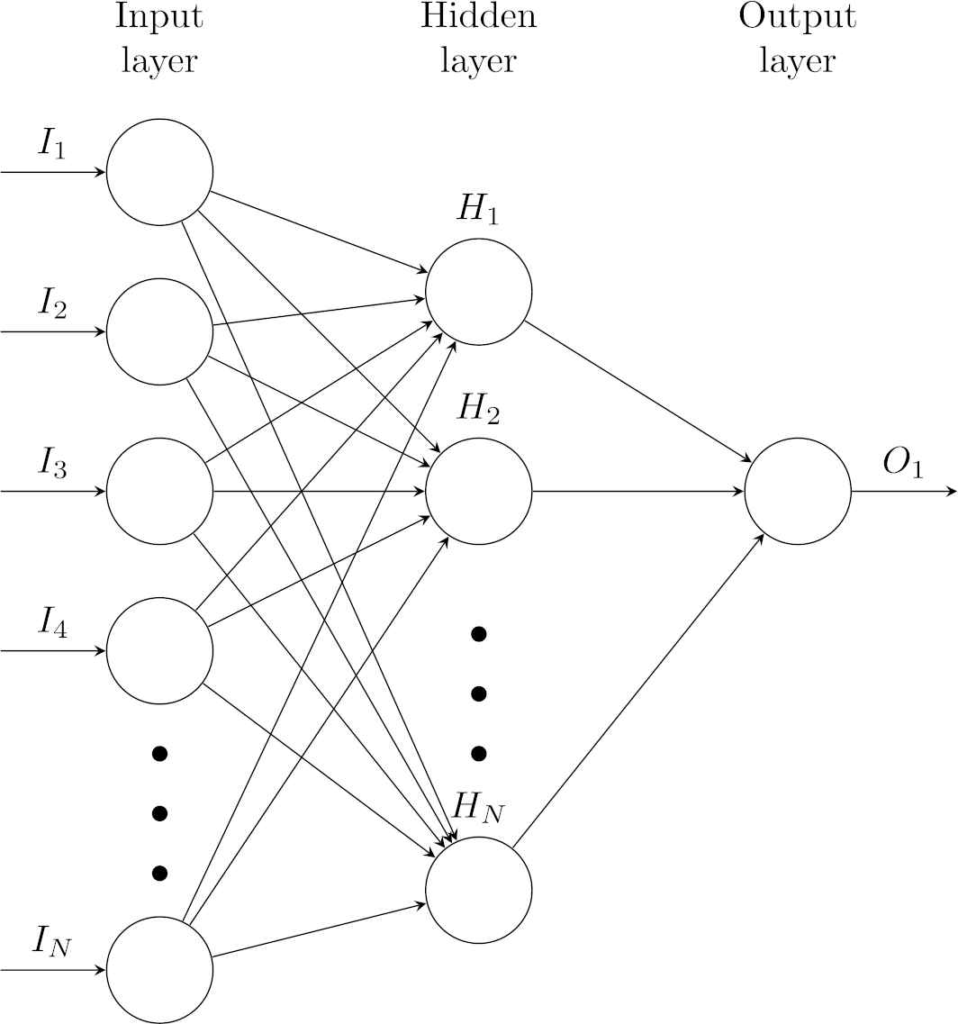
Feed-forward artificial neural network [37].
In general, the number of nodes and layers depend on experience and the level of understanding in the problem of the architect because so far, there is no theory for selecting the best parameters for ANN models. Hence, a fashionable approach is the trial and error until obtaining the appropriate parameters [13,38].
At each node (Fig. 2), the relationship of the input and the output can be expressed by
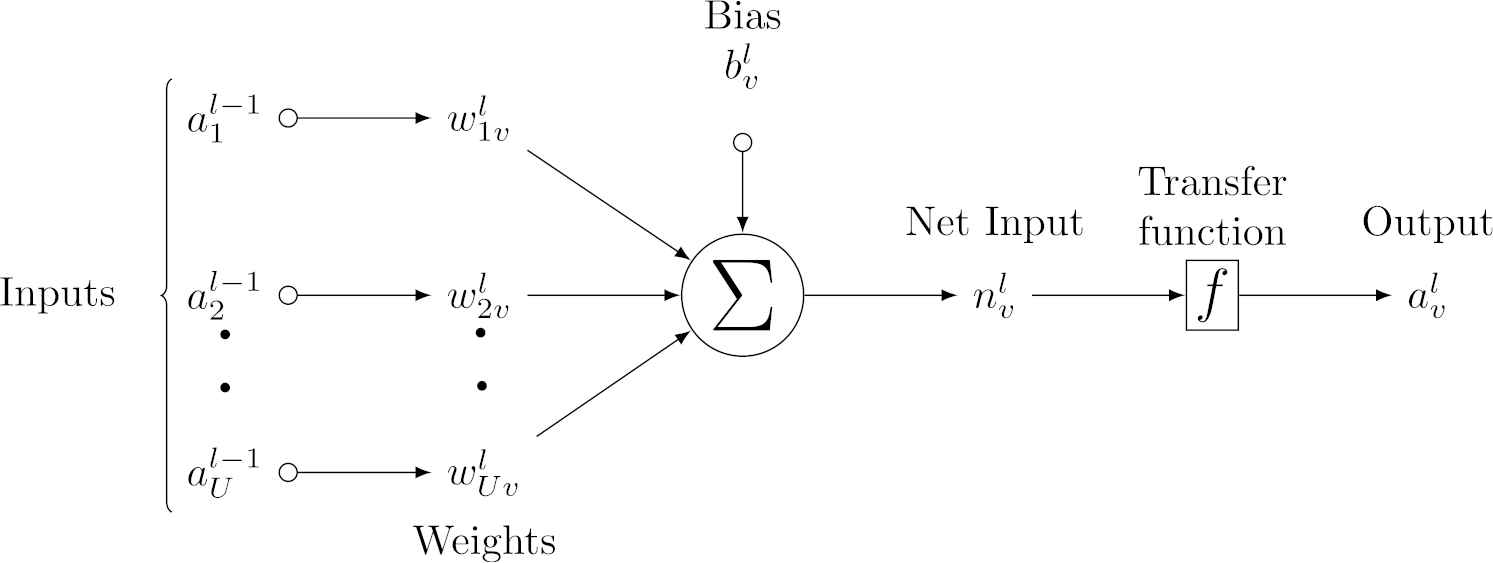
A node in artificial neural network [37].
For example, at node
After the output of the ANN model (e.g., forecasted export) is generated from the output layer, the output is compared to the target (e.g., actual export) to measure prediction accuracy. The ANN model can learn for minimizing the forecasting error via a training algorithm attempting to determine the weight (
In this research, a feed-forward ANN [37] is applied for the cassava starch export forecasting. The training algorithm is Levenberg-Marquardt algorithm with Bayesian regularization [39]. The idea of how to construct the ANN model for the cassava starch export forecasting in this paper is inspired by Pannakkong et al. [5] with an extension of the experimental scenarios. The following sections explain how the structure of the ANN model is identified.
3.2.1. Input layer
The input layer consists of the input nodes representing input variables (e.g., historical export quantity). Theoretically, the input variables can be divided into two types: technical variables and fundamental variables [38]. The technical variables are lagged values (e.g., time series value at time
In this study, there are totally nine input variables; six of them are the technical variables: three lagged values at time
In the experiments, there are three input scenarios that are designed based on the different combination of these nine inputs. The first input scenario is to include all nine inputs into the ANN model. For the second input scenario, the correlation analysis is performed first to screen the variables that have a statistically significant correlation (P-value
| Scenario 1 | Scenario 2 | Scenario 3 |
|---|---|---|
| All | Correlated | Time indices |
| Sequence | Sequence | Sequence |
| Month | Month | |
| Quarter | Quarter | |
| MA(3) | ||
| MA(12) | ||
| MA(3) | Seasonal index | |
| MA(12) | ||
| Seasonal index |
ANN inputs for native starch and modified starch.
| Scenario 1 | Scenario 2 | Scenario 3 |
|---|---|---|
| All | Correlated | Time indices |
| Sequence | Sequence | Sequence |
| Month | MA(3) | Month |
| Quarter | MA(12) | Quarter |
| Seasonal index | ||
| MA(3) | ||
| MA(12) | ||
| Seasonal index |
ANN inputs for Sago.
3.2.2. Output layer
The output layer is the layer that produces the results of the ANN model by aggregating the outputs from the hidden layer as:
3.2.3. Hidden layer
The hidden layer, the middle layer between the input and the output layers, generates the outputs by aggregation of the outputs from the previous layer with the weights, the biases, and the nonlinear transfer function, like the following:
In this study, only one hidden layer is used; however, the number of hidden nodes is varied from one to 20 nodes. Thus, totally, there are 180 ANN models constructed based on three types of the cassava export, three scenarios of the inputs and 20 scenarios of hidden nodes.
3.3. Khashei and Bijari's Hybrid Model
Generally, time series in real-world applications are rarely to have only pure linear or nonlinear characteristics [14]. In this case, the capability of the single forecasting models may not be enough to capture the relationship between the historical and future time series.
To overcome this circumstance, Zhang [14] has developed a hybrid model of the ARIMA and the ANN models in order to obtain capability in linear and nonlinear modeling from the ARIMA and the ANN modes respectively. However, in the Zhang's model, the relationship between linear and nonlinear components is assumed to be additive. This assumption may reduce the prediction accuracy of the Zhang's model if the relationship does not satisfy the assumption. Moreover, in some cases, the single forecasting models can perform even better than the Zhang's model [40].
Recently, Khashei and Bijari [15] modified the Zhang's model by proposing a novel hybrid model that defines time series as a function of its linear and nonlinear components. This relationship can be formally formulated as:
This hybrid model includes three stages: 1) extracting linear component (
In the first stage, the ARIMA model is applied to time series as presented in Section 3.1. The results of the ARIMA model are considered as the linear component of the time series.
In the second stage, Khashei and Bijari assumes that the nonlinear pattern still exists in the ARIMA residuals and the time series. Thus, the nonlinear components are defined as the functions of the lagged values of the ARIMA residuals and the lagged values of the time series as (
In the third stage, the time series can be represented by the function of the linear and the nonlinear components as:
Furthermore, seasonal ANN (SANN) can be employed in the Khashei and Bijari's model rather than typical ANN. The SANN captures seasonal nonlinear patterns in data from values of the same period in the pervious cycle(s). Therefore, the Khashei and Bijari (seasonal) model can be derived as:
4. PROPOSED HYBRID MODEL
In Pannakkong et al. [5], we have applied the ANN model for the cassava starch export forecasting which yielded a better accuracy than the ARIMA model. As discussed above, the hybrid models such as the Zhang's hybrid model [14] and the Khashei and Bijari's hybrid model [15] involve only lagged values of the time series for the prediction which may be inadequate for capturing complicated patterns in time series.
In the following, we develop a novel hybrid ARIMA and ANN model by further incorporating the MA and the seasonal index into the model, as graphically depicted in Fig. 3. The MA are the averages of previous

The proposed hybrid combining autoregressive integrated moving average (ARIMA) and artificial neural network (ANN) model.
The seasonal index is the ratio between the time series at considered period and the average of all time series in the cycle. If the time series value in a period is higher than the average value of its cycle, its seasonal index will be greater than one. Conversely, the seasonal index will be lower than one when the time series value is lower than the average value of its cycle. The number of periods for each cycle is the length of the cyclic pattern that can be identified by autocorrelation analysis of the time series. Usually, time series related to agriculture have the cyclic pattern every 12 months as they are affected by seasonal weather. The seasonal index can be computed as below:
The proposed model starts with separating the cassava time series into the training and testing set. Then, the linear and nonlinear components of the training set are determined as in the Khashei and Bijari's model.
Additionally, instead of taking only lagged values of time series into consideration, our proposed model also includes the correlated input variables shown in the second column of Tables 1 and 2 (denoted by
In time series forecasting problem, the number of input nodes corresponds to the number of the lagged values, which is used to discover the underlying pattern in a time series and to make forecasts for future values [13]. Therefore,
To determine the appropriate parameters of the proposed model, firstly, the results of the ARIMA model are generated as discussed in Section 3.1 and their residuals are computed. Secondly, the suitable
5. EXPERIMENTAL RESULTS
5.1. Cassava Starch Export Time Series
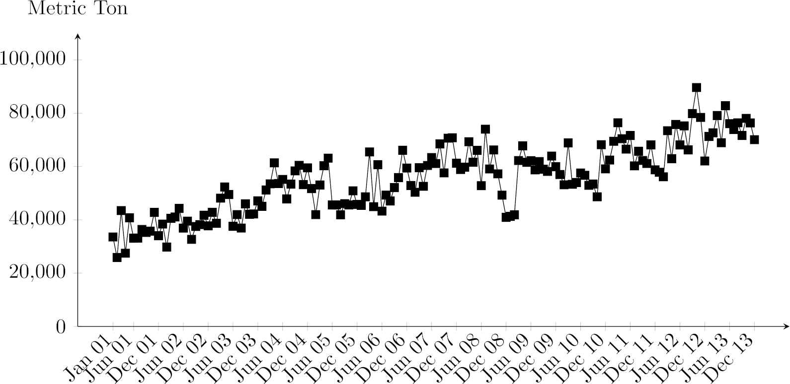
The cassava starch export time series contains monthly historical records of three types of the cassava export (i.e., native starch, modified starch, and sago) for 13 years (2001–2013). In term of average export quantity, the native starch is the first rank followed by the modified starch and the sago. In addition, these time series are nonstationary because their mean and variance are not constant as implied in Figs. 4–6.

Native starch time series.
Modified starch time series.
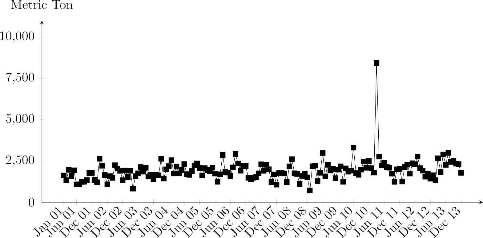
Sago time series.
There is uncertainty in the time series of cassava export quantity. In the long term, the cassava export quantity is increased due to the world's population growth and need for alternative energy resources. In short term, within a year, there is somewhat annual seasonality in the cassava time series due to the relevant events which are usually repeated annually such as seasonal weather, environmental issues (e.g., drought and pests), annual cassava pawn policy of the government, selling whole pawned cassava stock of the government in every September, and farmers' behaviors in the harvesting cycle.
Data partitioning is required to split the time series into training set and test set. The training set contains 144 monthly data during 2001-2012. The test set involves 12 monthly data in 2013 which is an unknown future for the forecasting models.
5.2. Forecasting Accuracy Measures
To measure the forecasting accuracy, three popular measures, namely mean square error (MSE), mean absolute error (MAE) and MAPE, are computed as in (20–22) respectively. Let
5.3. Forecasting Performance Comparison
After the comprehensive experimental runs, the forecasting accuracy measures are computed and compared in order to find out a suitable prediction model for each cassava starch. The MSE, MAE and MAPE of the best models in each type of forecasting model and each cassava type are presented in Tables 3 and 4.
| Cassava Export | Forecasting Model | MSE | MAE | MAPE (%) |
|---|---|---|---|---|
| ARIMA (1, 1, 0)(0, 1, 1) |
501,751,335 | 16,699 | 13.96 | |
| Native Starch | ANN (7-15-1)b | 2,383,777 | 1,091 | 1.10 |
| Khashei and Bijari [15] |
432,234,143 | 15,411 | 13.07 | |
| Khashei and Bijari [15] |
425,421,264 | 15,226 | 12.29 | |
| Proposedb |
87,655,928 | 7,522 | 6.60 | |
| ARIMA (0, 1, 3)(1, 0, 1) |
41,578,514 | 5,186 | 9.84 | |
| Modified Starch | ANN (9-19-1)a | 3,948,821 | 1,464 | 2.75 |
| Khashei and Bijari [15] |
27,960,066 | 4,221 | 7.79 | |
| Khashei and Bijari [15] |
42,033,243 | 5,220 | 9.34 | |
| Proposeda |
116,941 | 247 | 0.49 | |
| ARIMA (0, 0, 1)(1, 0, 0) |
490,409 | 370 | 19.70 | |
| Sago | ANN (4-6-1)b | 19,679 | 111 | 6.03 |
| Khashei and Bijari [15] |
51,479 | 167 | 9.74 | |
| Khashei and Bijari [15] |
998,749 | 617 | 33.95 | |
| Proposedb |
9,529 | 73 | 4.04 | |
ANN, artificial neural network; ARIMA, autoregressive integrated moving average; MAE, mean absolute error; MAPE, mean absolute percentage error; MSE, mean square error.
With technical and fundamental inputs.
With significant correlated inputs.
Training performance of cassava export forecasting.
| Cassava Export | Forecasting Model | MSE | MAE | MAPE (%) |
|---|---|---|---|---|
| ARIMA (1, 1, 0)(0, 1, 1) |
2,954,264,813 | 46,344 | 21.02 | |
| Native Starch | ANN (7-15-1)b | 978,697,046 | 23,738 | 12.19 |
| Khashei and Bijari [15] |
1,186,289,692 | 27,565 | 14.95 | |
| Khashei and Bijari [15] |
2,807,270,432 | 45,063 | 20.58 | |
| Proposedb |
631,588,845 | 19,462 | 10.79 | |
| ARIMA (0, 1, 3)(1, 0, 1) |
25,259,327 | 4,513 | 6.06 | |
| Modified Starch | ANN (9-19-1)a | 16,987,064 | 3,185 | 4.25 |
| Khashei and Bijari [15] |
21,870,151 | 3,797 | 5.01 | |
| Khashei and Bijari [15] |
34,223,857 | 5,032 | 6.64 | |
| Proposeda |
12,628,092 | 2,893 | 3.84 | |
| ARIMA (0, 0, 1)(1, 0, 0) |
306,717 | 460 | 19.54 | |
| Sago | ANN (4-6-1)b | 191,042 | 319 | 13.41 |
| Khashei and Bijari [15] |
131,358 | 302 | 12.44 | |
| Khashei and Bijari [15] |
270,294 | 453 | 20.08 | |
| Proposedb |
229,176 | 369 | 16.10 | |
ANN, artificial neural network; ARIMA, autoregressive integrated moving average; MAE, mean absolute error; MAPE, mean absolute percentage error; MSE, mean square error.
With technical and fundamental inputs.
With significant correlated inputs.
Testing performance of cassava export forecasting.
The best model for the native starch is the proposed model followed by the ANN model, the Khasei and Bijari's model and the ARIMA model. From Fig. 7, The ANN is more accurate than the proposed in January to June. On the other hand, the proposed model outperforms the ANN in July to December. The ARIMA underestimates the actual export in all month except June. The Khasei and Bijari's model can capture the actual trend roughly.
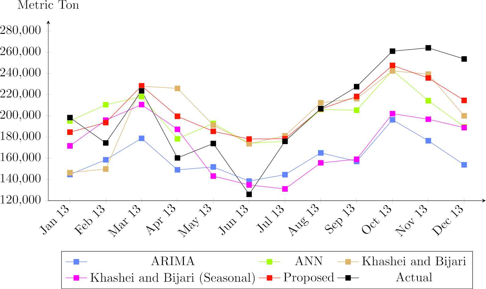
Forecasting export comparison for native starch.
For the modified starch, the proposed model is the best model followed by the ANN model, the Khasei and Bijari's model [15] and the ARIMA model respectively. From January to May, all models can capture the direction of the future export except the ARIMA model in May (see Fig. 8). After May, the forecasting direction seems to be opposite to the actual value until October but in November and December, all models give the same forecasting direction.

Forecasting export comparison for modified starch.
In the case of the sago, surprisingly, the best model is the Khasei and Bijari's model [15] followed by the ANN model, the proposed model and, the ARIMA model respectively. The Khasei and Bijari's model [15] can obviously track the direction of the future export from January until June. The other models can track the direction only in January, March, and April (see Fig. 9). In addition, the ANN and the proposed model perform almost the same. The ARIMA model gives somewhat similar values for the whole year. It seems that the 12 lagged values in the Khashei and Bijari's model can cover the pattern the time series of the sago. Therefore, including the correlated variables into the model incurs overfitting of the historical time series (i.e., training set).
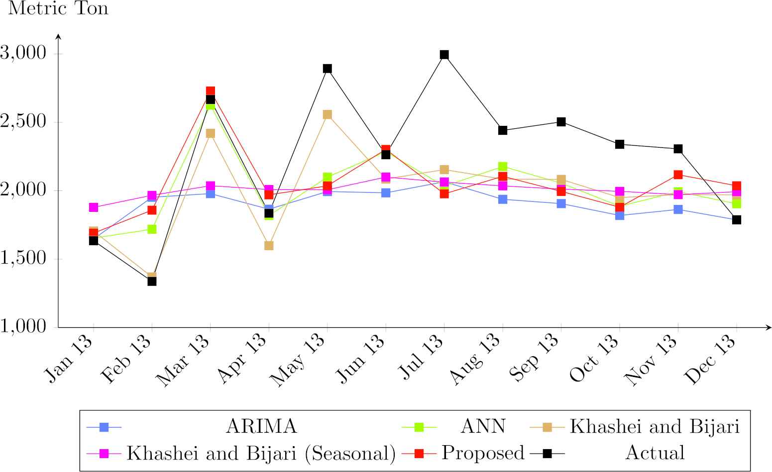
Forecasting export comparison for sago.
From the overall results, prediction accuracy in testing is worse than training except for the ARIMA and seasonal Khashei and Bijari's models in sago prediction. The ARIMA model has almost similar MAPE in both training and testing because it is robust for the outlier in testing set of the sago. The seasonal Khashei and Bijari's model in testing gives better performance than training, however, its performance is still the worst among all forecasting models as the sago time series has no obvious seasonality.
In training, the proposed model performs the best in all types of the cassava starch except the native starch. The ANN model has 1.10% of MAPE following by the proposed model having 6.60% of MAPE. However, in testing, MAPE of the ANN model increases by 12 times (13.41% of MAPE) approximately while MAPE of the proposed model increases by less than 2 times (10.79% of MAPE). This evidence implies that the overfitting problem occurs during the training of the ANN model.
The seasonal Khashei and Bijari's model has less accurate prediction than typical Khashei and Bijari's model because the cassava export time series are not pure seasonal time series and the seasonal Khashei and Bijari's model can capture only the seasonal pattern from SARIMA and SANN without obtaining recent information from recent lagged values. However, typical Khashei and Bijari's model obtains seasonal pattern from SARIMA and also receives the pattern within cycle from recent lagged values.
In summary, for the reason that the proposed model outperforms the Khashei and Bijari's model [15] in predicting the native starch and the modified starch, there may be remaining nonlinear component that cannot be captured with the residuals of ARIMA and the lagged values but it can be captured in which the correlated inputs are included in the model. On the other hand, the Khashei and Bijari's model [15] is the best model for the sago because the proposed and the ANN models, which are more complex in term of inputs, give more weight to an extreme outlier that causes the overfitting problem as the proposed model has the best performance in training stage (Table 3).
6. EXPERIMENTS WITH OTHER SEASONAL TIME SERIES
The previous section implies the capability of the proposed model in cassava export forecasting. However, the structure of the proposed model is not limited for only cassava export time series. This section illustrates the effectiveness of the proposed model to the other two seasonal time series (i.e., milk production and temperature).
The monthly milk production time series [41] was collected during January 1962 to December 1975 (168 observations) as shown in Fig. 10. The cyclic pattern is obviously repeated annually. It has an increasing trend from 1962 to 1971. After that, the production mean seemed to be stable. The observations from 1962 to 1974 are used in the training stage. The remaining observations in 1975 are testing data.

Milk production time series.
The mean daily temperature of Fisher River near Dallas [42] was continuously recorded from 1988 to 1991. The daily observations are aggregated into 48 monthly observations as presented in Fig. 11. The mean of temperature is quite stable during these four years. The peak of temperature usually occurs in the middle of the year. However, the patterns in each year are slightly different. The first three years (1988 to 1990) observations are training set. The testing set is observations in 1991.
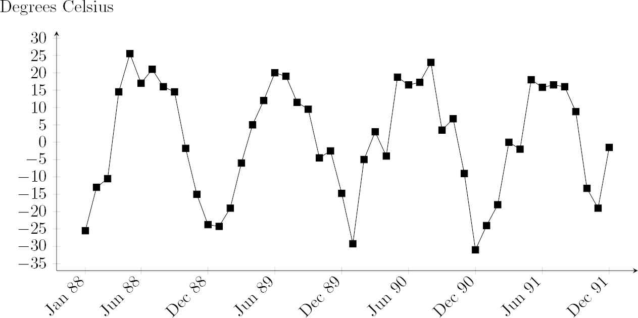
Temperature time series.
The correlation analyses are performed to find their significant correlated inputs as presented in Table 5. After these two time series are analyzed by the proposed model and benchmarking models, the performance in training and testing is shown in Tables 6 and 7. The forecasting values are plotted in Figs. 12 and 13.
| Milk Production | Temperature |
|---|---|
| Sequence | Month |
| Quarter | |
| MA(3) | MA(3) |
| MA(12) | MA(12) |
| Seasonal index | Seasonal index |
Significant correlated inputs for milk production and temperature.
| Time Series | Forecasting Model | MSE | MAE | MAPE (%) |
|---|---|---|---|---|
| ARIMA (0, 1, 1)(0, 1, 1) |
55.71 | 5.71 | 0.77 | |
| Milk Production | ANN (7-10-1)a | 5.19 | 1.75 | 0.24 |
| Khashei and Bijari [15] |
12.15 | 2.33 | 0.31 | |
| Khashei and Bijari [15] |
44.66 | 4.85 | 0.64 | |
| Proposeda |
11.72 | 2.32 | 0.30 | |
| ARIMA (0, 0, 0)(0, 1, 0) |
9.78 | 2.39 | 127.14 | |
| Temperature | ANN (7-2-1)a | 0.35 | 0.47 | 31.64 |
| Khashei and Bijari [15] |
2.68 | 1.14 | 94.19 | |
| Khashei and Bijari [15] |
6.63 | 1.92 | 52.40 | |
| Proposeda |
2.44 | 1.05 | 92.08 | |
ANN, artificial neural network; ARIMA, autoregressive integrated moving average; MAE, mean absolute error; MAPE, mean absolute percentage error; MSE, mean square error.
With significant correlated input.
Training performance of milk production and temperature forecasting.
| Time Series | Forecasting Model | MSE | MAE | MAPE (%) |
|---|---|---|---|---|
| ARIMA (0, 1, 1)(0, 1, 1) |
160.65 | 10.99 | 1.28 | |
| Milk Production | ANN (7-10-1)a | 169.22 | 11.46 | 1.35 |
| Khashei and Bijari [15] |
147.07 | 10.77 | 1.24 | |
| Khashei and Bijari [15] |
156.32 | 11.59 | 1.34 | |
| Proposeda |
132.55 | 10.58 | 1.22 | |
| ARIMA (0, 0, 0)(0, 1, 0) |
17.24 | 3.35 | 949.43 | |
| Temperature | ANN (7-2-1)a | 11.21 | 2.75 | 839.90 |
| Khashei and Bijari [15] |
16.56 | 3.30 | 141.77 | |
| Khashei and Bijari [15] |
28.43 | 4.90 | 803.96 | |
| Proposeda |
16.05 | 3.25 | 120.47 | |
ANN, artificial neural network; ARIMA, autoregressive integrated moving average; MAE, mean absolute error; MAPE, mean absolute percentage error; MSE, mean square error.
With significant correlated input.
Testing performance of milk production and temperature forecasting.
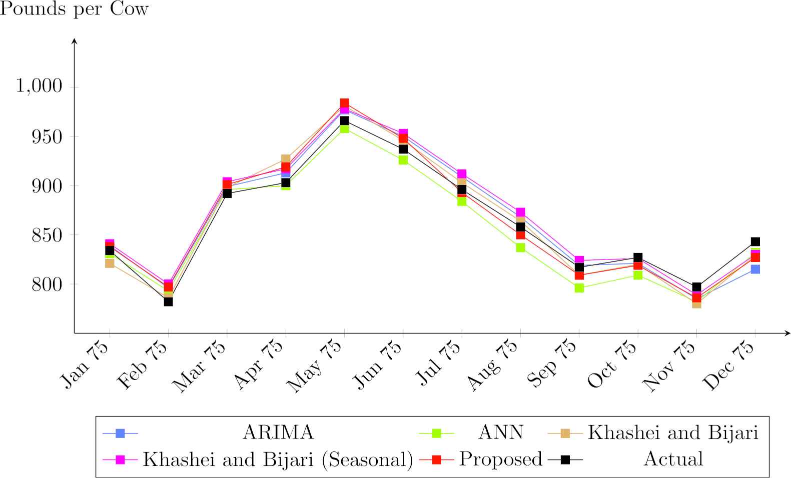
Forecasting comparison for milk production.
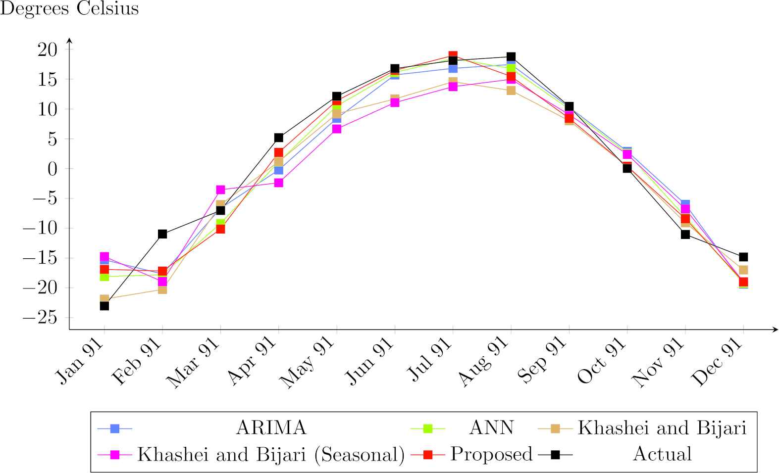
Forecasting comparison for temperature.
From the results, there are some interesting points to be noted. Training performance is better than testing performance because test data set in unknown for the prediction models. ANN gives the best performance in training for both milk production and temperature.
Training and testing MAPEs of milk production are not quite different. Conversely, in case of temperature, testing MAPE of some models is dramatically increased from training MAPE. The reason is that MAPE is sensitive when mean of data set is low. Mean of temperature is very low (approximately zero), therefore small predict error can cause huge changing in MAPE.
Considering the testing performance, they indicate that the proposed model outperforms all benchmarking models in milk production forecasting with lowest error in all three measures. For temperature forecasting, the proposed model can perform the best in only MAPE and give the second-lowest MSE and MAE, while ANN has the lowest MSE and MAE. This result implies that when mean of data set is very low, both the proposed model and ANN should be applied and then their results should be compared based on user preferences.
7. CONCLUSION
In recent years, hybridization of the ARIMA and the ANN models have been proved to often provide a more accurate prediction than individual models used separately. However, there is a limitation regarding the input adequacy of previously developed hybrid models. In this paper, we proposed a new hybrid model for the cassava export forecasting, which also combines the ARIMA model and ANN and additionally considers the MA and the annual seasonal index along with the lagged values of the time series as the inputs for fitting the nonlinear relationship. After conducting the comprehensive experiments, the prediction performances of the proposed hybrid model are compared to the ones by the ARIMA model, the ANN model and the Khashei and Bijari's model [15].
In conclusion, the proposed model shows its capability in the cassava export forecasting with the highest accuracy in MSE, MAE, and MAPE comparing with the ARIMA model, the ANN model, the Khashei and Bijari's model and the seasonal Khashei and Bijari's model in case of the native starch and the modified starch. However, for sago, the Khashei and Bijari's hybrid model is the best. Although, the proposed model is not suitable for sago, it can give the most accurate forecast for the native starch and the modified starch which covers around 98% of the total export volume.
Regarding the capability of the proposed model, it can contribute the cassava international trading market as an alternative forecasting model for the major volume of the cassava export. The forecasting results from the proposes model would be useful for the stakeholders who make a decision based on the future cassava starch export. Furthermore, as the cassava is a seasonal time series, this hybrid model can be applied to other seasonal time series that share the similar characteristic as it provides the best performance in all three measures in predicting milk production, and the best MAPE in predicting temperature.
Nevertheless, the experiments conducted are limited to 12 months ahead prediction, three replication runs for each scenario, one hidden layer and twenty hidden nodes. In future work, we intend to apply a technique (e.g., response surface methodology) to find optimal hyperparameters rather than trial and error to obtain more reliable results, and also make an attempt to find out a solution to deal awith the outlier of the sago.
CONFLICT OF INTEREST
The authors confirm that all funding sources supporting the work and all institutions or people who contributed to the work, but who do not meet the criteria for authorship, are acknowledged. The authors also confirm that all commercial affiliations, stock ownership, equity interests or patent licensing arrangements that could be considered to pose a financial conflict of interest in connection with the work have been disclosed.
AUTHORS' CONTRIBUTIONS
W. Pannakkong and V.N. Huynh conceived of the presented idea. W. Pannakkong developed the proposed model and performed the experiments. V.N. Huynh and S. Sriboonchitta supported W. Pannakkong in verifying the analytical methods. All authors discussed the results, provided critical feedback, and helped shape the research, analysis, and manuscript. W. Pannakkong and V.N. Huynh wrote the manuscript in consultation with S. Sriboonchitta. V.N. Huynh sent the manuscript for publication and communicated with the journal editor.
Funding Statement
This work was supported by the SIIT Young Researcher Grant, under contract no. SIIT 2017-YRG-WP05.
ACKNOWLEDGEMENTS
The authors would like to thank the anonymous reviewers for providing insightful comments and providing directions for additional work which has resulted in this paper. This work was supported by the SIIT Young Researcher Grant, under contract no. SIIT 2017-YRG-WP05.
REFERENCES
Cite this article
TY  - JOUR
AU  - Warut Pannakkong
AU  - Van-Nam Huynh
AU  - Songsak Sriboonchitta
PY  - 2019
DA  - 2019/09/26
TI  - A Novel Hybrid Autoregressive Integrated Moving Average and Artificial Neural Network Model for Cassava Export Forecasting
JO  - International Journal of Computational Intelligence Systems
SP  - 1047
EP  - 1061
VL  - 12
IS  - 2
SN  - 1875-6883
UR  - https://doi.org/10.2991/ijcis.d.190909.001
DO  - 10.2991/ijcis.d.190909.001
ID  - Pannakkong2019
ER  -