1. INTRODUCTION

With the development of social economy, it is an important task for every coastal country to monitor and identify the Marine vessels, for it plays an important role in protecting Marine resources, monitoring and managing fishing boats, fighting against smuggling and so on. Exact detection and identification of ships can help to better monitor the water transport. An optimized ship identification system can effectively improve the shipping environment, maintain the maritime traffic order, fully enhance the operational capacity of the port and reduce the traffic accidents. In addition, ship identification technology has military strategic significance for accurately tracking the ship targets and realizing the precision guidance [1].

Until recent years, ship identification technology has not yet got popularized. The common method involves preprocessing, feature extraction and classifier. The main defect of this method is that it needs complex image processing algorithm but cannot get a satisfactory experimental result. In addition, convolutional neural network (CNN) is also well applied to the ship identification. However, the latest data shows that the identification accuracy is not ideal [2], hence it is extremely urgent to improve the identification accuracy. Ship identification is also one of the research hotspots in the field of pattern recognition. In 2014, Jiang Shao Feng et al. proposed Synthetic Aperture Radar (SAR) commercial ship classification algorithm based on structural characteristics [3], which can classify bulk cargo ships, container ships and fishing boats. With the rise of method of neural network, Liang Jin Xiong used BP neural network to identify the infrared images of aircraft carriers, destroyers, frigates, passenger ships, container ships and oil ships in 2015 [4]. In 2016, Zhao Liang with his research team designed CNN for ship image classification, and acquired a better classification effect [5].

With the breakthrough of Deep CNN in image classification task, Jia Yangqing, as well as other scholars and researchers, has generated strong interest and devotion in it. Studies have shown that Deep CNN model which has been well systematically trained with ImageNet is used to extract deep convolution activation feature (DeCAF) [6]. When combined with different classifiers, it is able to obtain great results in identifying various scenes and birds. The experiments show that the sixth layer, the fully connected layer (DeCAF6) based on AlexNet [7] network, is superior to other layers in both bird recognition and target recognition tasks. For this reason, AlexNet network is adopted and DeCAF is introduced to conduct network training for the data set of transport ships with complex background. Then, DeCAF6 features of the network are extracted. Combining with SVM classifier, this paper respectively classifies and identifies three types of transport ships with high similarity, namely container ships, bulk carriers and oil and gas ships. The CNN architecture proposed by Krizhevsky et al. [8] has made a great breakthrough in Image-net Large Scale Visual Recognition Challenge (ILSVRC2012) (In the image classification task, the performance is 10% higher than that of the traditional feature architecture). Subsequently, Razavian et al. [9] pointed out that the CNN model obtained through pre-training on the large-scale image library could be used to extract the visual features of images and applied to various image recognition tasks, such as scene classification and multi-tag classification. Ma Xiaofeng et al. [10] proposed an attention-based mechanism to extract environmental features by adding a fully convolutional network (FCN) branch to the detection network. Yu Zhang et al. [11] proposed a method to adjust the parameters such as the size of region proposal network (RPN) anchor and threshold value of non-maximum suppression (NMS), so as to improve the certainty of image mask extraction in multi-target scenes. However, when these models are applied to ship image recognition in real complex situations, there are still some problems in precision, quality and accuracy, where there is a gap from the idealized requirements of actual application. In the field of pattern recognition, ship image recognition has been one of the main points researchers focused on. By means of Segmentation and Artificial Neural Network, G.K. Yuksel [12] provided a way out to extract ship characteristics and identify ships from three-dimensional (3D) ship silhouette image. K. Rainey et al. [13] put forward the CNN for ship identification, and Corbane et al. [14] detected small ship targets by wavelet transform and radon transform of satellite images. The experiments on satellite ship images show that the recognition results are good.

Although these existing studies have acquired good recognition effect, they mainly focus on the ship images with large shape differences in a single background. Because of the complex backgrounds, small differences in hull shapes and the shooting angles, a large number of images of transport ships taken in real ports and waterways are of high similarity, making the traditional method of classification and identification for ship images unable to gain good results. How to improve the effect of this kind of ship image recognition is a difficult problem in the research of ship image recognition. In order to make up for the above shortcomings and to solve the related problems, this paper proposes a vessel target positioning and mask generation algorithm based on Mask RCNN [15], which has strong detection performance for Marine vessels and greatly enhances the accuracy and practicability of the algorithm. It has important theoretical and applied value to people's livelihood, economic construction, fishery administration supervision, maritime traffic management and even military field.

In the detection of offshore vessels, the experimental results show that the improved Mask RCNN model achieves better performance and higher precision than the existing deep learning vessel detection technology in a relatively short time.

2. RELATED WORK

The main idea of Mask RCNN is to locate multiple feature regions in an image, input each region into CNN for feature extraction [16] and generate a Mask on the feature-extracted region. The biggest feature of Mask RCNN is to separately extract the classified regression information of the image to be tested (that is, the border information of the target to be tested) and combine it with the pyramid features (the length and width of the image input for pyramid region of interest [ROI] processing, that is, PyramidROIAlign) for mask generation, which is shown in Figure 1.

Figure 1

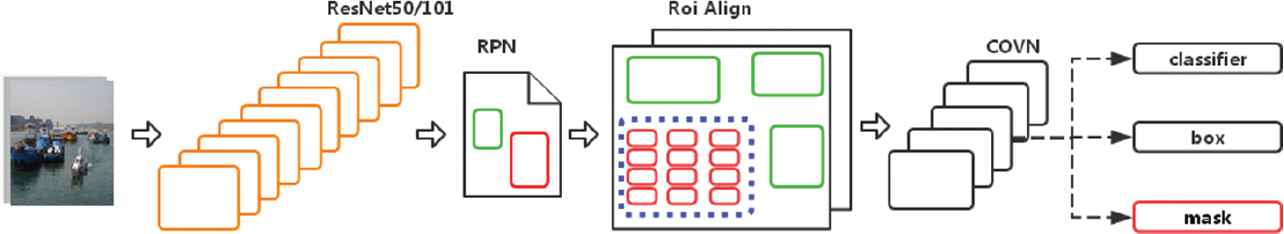
Mask RCNN model.

In the ship target positioning Mask RCNN architecture, ResNet works as the backbone network for feature mapping and FCN works as the backbone network for Mask prediction. According to the principle of network effect, “the deeper, the better,” ResNetXt-101 is adopted in this paper as the basis of backbone network, and ROI Align layer is employed to alight the extracted features with the pre-input [17]. ROI Align layer can accurately locate the ship targets, which is very important in the Mask RCNN system. In this paper, CNN is connected to the back of the ROI Align layer to extract the input features for classification and mask generation. Ship classification gets the alignment feature map of 7*7 from the ROI Align layer, and ship mask generation gets the alignment feature map of 14*14 from the ROI Align layer. In addition, CNN is composed of four convolution layers and two fully connected layers, each convolution layer of which is followed by Relu activation and maximum pooling sampling. Finally, the loss function output of Mask RCNN is as follows:

In Formula (1), L_cls, L_box and L_mask refer to classified loss function, prediction box loss function and mask loss function respectively.

3. REGION PROPOSAL NETWORK (RPN)

In fact, RPN is a core network of Mask RCNN (as shown in Figure 2), which is an important leading step to realize FPN feature layer selection and ROI Align. RPN is the FCN, which can conduct end-to-end training for the mission to generate testing suggestion box. Therefore, it can predict the boundary of the target and the score at the same time, as long as two extra full convolution layers (Cls-Layer and Reg-Layer) are added. Reg-Layer is used to predict the coordinates x, y, width w and height h of the feature region corresponding to the center anchor, while Cls-Layer is used to determine whether the feature region is the foreground or the background. The sliding window processing method can ensure that Reg-Layer and Cls-Layer are associated with all feature spaces.

Figure 2

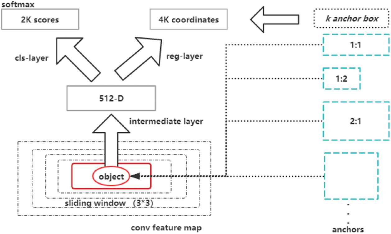
Region proposal network (RPN) structure.

When inputing a convolution layer of 3*3*512*512 to the RPN network, we will get an output of 11*11*512, where 11*11 represents the size of feature region. It is assumed that there are several 11*11 big black boxes in the original image. Each of them has nine little color boxes and 3*3 = 9 anchors. The anchors are located in the center of the 3*3 sliding window. We can predict multiple feature regions through one sliding window. If there are k feature regions (that is, k reference frames), then each reference frame can be confirmed by the size, ratio and uniqueness of the anchor points in the sliding window. An anchor can refer to an anchor box or a reference frame. If k = 9, it indicates three dimensions (128², 256², 512²) and three ratios (1:1, 1:2, 2:1) [18]. When nine reference frames corresponding to the current sliding window position are identified, the W*H feature map and its corresponding W*H*k anchors will bear the scale invariance (as shown in Figure 3), which can produce the boxes with a certain ratio of 11*11*9 at different positions. This is enough to pinpoint all target objects. If it is assumed that there is a target object in the original image, it can be located in the frame simply by translating the black box.

Figure 3

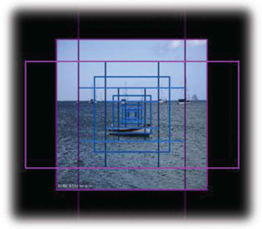
Generation of nine anchor boxes.

4. LOSS FUNCTION

In this paper, the calculation rules of Loss function are set as follows:

1. The positive and negative sample calibration rules of anchors must be set before calculating the loss. Assuming that the intersection over union (IOU) between the reference box and ground truth (GT) of Anchor was greater than 0.7, it is marked as a positive sample; and when the overlap (IOU) between the reference box and GT of Anchor is less than 0.3, it will be marked as a negative sample. As for the remaining samples that are neither positive nor negative, they will not participate in the final training [19].

2. The loss function of training RPN includes regression calculation loss and classification loss (ithat is, Softmax loss).

In this paper, the gradient method combining norm L1 with norm L2 is used to solve the problem that the gradient value will not be too large when the difference between the prediction box and the GT is too large and can be small enough when the difference is very small. When the input x is less than 1, norm L1. (Formula 2) is used to make the gradient smoother and easier to differentiate. When the input x is greater than 1, norm L2 (Formula 3) is used to effectively avoid the gradient explosion and reduce the outliers.

The detection block location of loss function is set as Lloc, the predicted translation and scaling parameter is set as tu, and the actual translation and scaling parameter is set as v. Thus the loss rate of detection block location is evaluated by comparing the difference between the two parameters, which is as shown in Formula (4).

The loss rate of RPN is obtained by Formula (2), Formula (3) and Formula (4). In Formula (5), pi refers to the probability that the i-th anchor is a target object. When the target is found, pi is 1; otherwise, pi is 0. ti is the four coordinate parameters of the boundary box (t_x, t_y, t_w, t_h) when predicting RPN, which corresponds to the coordinates of positive anchor point GT. Lcls is the loss function of dichotomy (target/non-target), and Lreg is the loss function of smoothL(1,2), which is used to predict boundary box and GT box._. The normalized total loss rate of RPN is obtained by the combination of Ncls, Nreg and λ (balance weight). Through trial and error, we find that setting λ to 10, Ncls to 512 and Nreg to 2500 can keep the balance of loss values of the two parts of RPN. Finally, a series of feature regions are acquired by RPN through training.

5. ROI ALIGN

The feature region obtained by RPN processing is processed by ROI Align, so that it can provide required ROI input for mask generation. ROI Align is the improvement of ROI Pooling of Fast RCNN. ROI Align cancels the quantization operation. For the pixel whose coordinates are floating point numbers in the quantization, bilinear interpolation is used to calculate the pixel value, so as to prevent the loss of some feature point information from later aggregation [20]. Through experiments, we find that ROI Align is obviously effective to enhance the dataset with a large number of close-up large objects. However, as for the the dataset with a larger number of long-range small targets, ROI Align does not work well. It is mainly because small targets are easier to be affected by non-linear problems (for example, for large targets, the deviation of 0.1 in pixel is insignificant, but for small targets, the impact of error is great). For the reasons above, the anchor point cannot locate the distant hull target in the generated top-level anchors, which is shown in Figure 4.

Figure 4

The generated top-level anchors.

In order to solve the above problem of small targets location, we make RPN generate a total of 261888 anchor points, and set the scale of the feature image as (32, 64, 128, 256, 512) and the proportion as [0.5, 1, 2]. When ResNet generates five different-scale feature maps, the trunk network will be input into the RPN network and respectively generate ROI. Then, the RPN network generates several Anchor-Boxes through these five feature maps of different scales. The number of anchor boxes is shown in Table 1.

In this paper, nearly 1000 ROIs are retained after the NMS operation (1000 is a variable parameter). Because of the difference in strides, ROI Align operation is performed on the stride corresponding to the Feature maps of five different scales [Level 1, Level 2, Level 3, Level 4, Level 5] respectively. The ROI generated after this operation is the combination of down-sampling and NMS, which solves the problem that small targets cannot be located in ROI Align. Through the above method, the generated ROI includes all target vessels in the figure (as shown in Figure 5), providing the accurate input source for the subsequent mask generation.

Figure 5

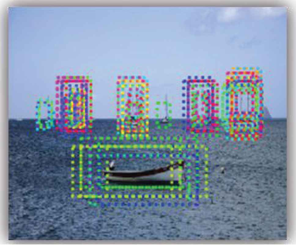
The region of interest (ROI) generated.

6. MASK GENERATION

The mask generation in the Mask RCNN is achieved by citing an additional network separately. This mask generation branch is a full-convolutional-neural networks, where the positive region selected by the ROI Align classifier is used as input to generate a mask of 14*14 low resolution pixels. The size of the mask is such small that it helps to keep the light weight of mask generation branch network. In the training process, we reduce the size of actual mask to 14*14 to calculate the loss function. In the inference process, we amplify the size of the predicted mask to the border of ROI, so as to get the final result of mask. The procedure of mask generation is shown in Figure 6.

Figure 6

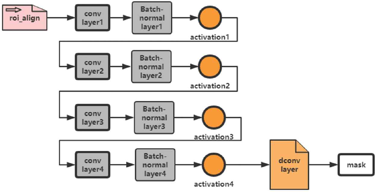
Process of mask generation.

Mask generation is mainly to add a series of convolution operations after ROI Align expands its output dimension, so as to predict the mask more accurately. The operating parameters are shown in Table 1. This process is conducted through the ROI feature map generated by many inputs of the same size in ROI Align. Each output channel has 256 fusion feature layers. The number of the outputs is 256 and the size is 14*14. As shown in Figure 3, the output is generated by one-way mask through four levels. Each level involves a convolution layer, a normalized layer and an activation function, which is finally connected to a deconvolution layer to acquire the mask.

The mask generated in the original model cannot be dynamically given in accordance with the target window. In the process of distant hull detection, mask generation branches cannot ensure the precise segmentation for instance, resulting in target loss or tiny interferences. To solve these problems, we propose an improved mask generation structure.

7. IMPROVED MASK STRUCTURE

In this paper, the mask branch is improved. After three times of convolution and aggregation, each ROI region x is shown as follows

Among them, wai,wbi,wci are the weight vectors, and b1j,b2j,b3j are the offset vectors. In this paper, a random gradient descent algorithm is used to minimize the expected risk. The cost function is as follows.

Therefore, the rule for updating the parameters of Random gradient descent (SGD) at this time is wj=wj+αyi−hwxixji, and the output results are upsampled and restored to get a new x′,x″, that is,

It is the upsampling function. After another convolution and pooling process, the output result f1(x),f2(x) is obtained by activating the linear rectifier (relu) function, which is shown as follows.

Among them,wci is the weight of the third convolution, bj is the bias quantity, and relu is the activation function. Finally, in order to obtain the segmentation result, the f1 (x) and f2 (x) are merged and multiplied by the shared weight λ obtained by the Time Distribution layer operation.

The structure is shown in Figure 7.

Figure 7

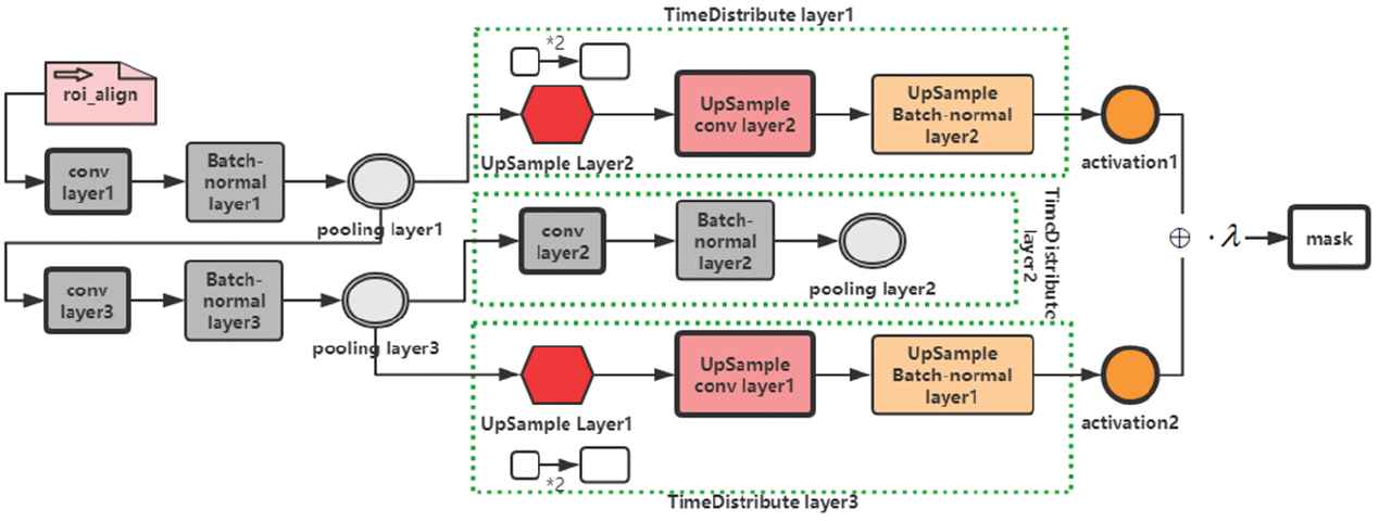
Process of the improved mask generation.

The improved mask generation process mainly better the mask segmentation effect of each ROI. The pooling layer 1 and 3 are connected, and the pooling layer 3, connected to the pooling layer 2, is the convolution of the pooling layer 1. The pooling layer 1 and 3 are connected to the upper sampling layer respectively, so as to constitute a Two-Way sampling. Finally, the two channels are activated and merged into one path and multiplied by a shared weight to generate a mask. With the use of two-way sampling, the feature information of the image increases while the dimension of image description does not increase on the premise that the number of channels remains unchanged. Increasing the amount of information per dimension only is obviously beneficial to the final mask generation.

7.1. Shared Weight Generation

Through the Time Distribution layer, the multi-layer convolution features of the RPN network output can be shared. Therefore, the real significance of Time Distribution is to share the weight among the feature maps of different levels. The Time Distribution layer applies mask generation branch to a specific vector and performs an operation on each vector without increasing the final output vector. The Time Distribution layer performs upsampling, convolution, normalization, pooling and other operations on each time slice. Through a series of operations, we get a result, that is, the shared weight. Shared weight generation is shown in Figure 8.

Figure 8

Shared weight generation.

In the process of mask generation improvement, through the operations of Time Distribution_Layer 1, Time Distribution_Layer 2 and Time Distribution_Layer 3, different time slices are defined as f1(x),f2(x),f3(x) to generate the output weight P1, P2, P3 respectively, and the output weight value is twice as much as its corresponding input weight, which is shown in Formula (11).

(11)P1=∑i2waixi+b1jP2=∑i2wbixi+b2jP3=∑i2wcixi+b3j

The Shared Weight λ required in Formula (11) is expressed as logPtft(x), as shown in the Formula (12)

(12)log⁡Ptft(x)=∑t=1NlogPtft(x)|  f1(x),f2(x),f3(x),…,fn(x)

8. EXPERIMENT

8.1. Dataset Preparation

The data set used in this experiment is the ship pictures crawled from the network by crawler program. Due to the image size requirement of Mask RCNN, the size of the data set image is 512*512. LabelMe is used to mark the area where the ship target is located in the image. LabelMe is an open annotation tool created by the Computer Science and Artificial Intelligence Laboratory of the Massachusetts Institute of Technology (MIT CSAIL) [21]. Through LabelMe software, it is convenient to mark and preserve the boundary of all kinds of ship targets in the image.

LabelMe generates label images, mask images and logo images (as shown in Figure 9). We have produced the Mask RCNN standard dataset 3000, which includes three kinds of ocean ship images: ocean-going cargo ship, inshore fishing boat and large warship.

Figure 9

Ship target marking.

8.2. Training

In this paper, the time of training cycle is set as 5, each cycle iterates 100 steps, and the number of training steps usually depends on the size of the dataset. It takes a big amount of memory resources and time for large-scale data set training to use the above model; therefore, it needs a high-end hardware. The hardware parameters involved in this paper are CPU: Intel (R) Core (TM) i7-6820HQ 8 core, Memory: 32G, and GPU: Nvidia Quadro M2000M; while the software environment is built with Python3, Keras2, TensorFlow1.4. Comparing with the previous Mask RCNN architecture, the improved Mask RCNN network training can optimize the training time, loss rate and so on, which is shown as follows. In this paper, four methods are used for training:

1. RPN _(L1) with L1 Norm and pre-improved mask (Mask _(O)) Generation method;

2. RPN with L1 Norm and improved Mask _(N) Generation method;

3. RPN _{(L1, L2)} with L1 and L2 Norm and pre-improved mask (Mask _(O)) Generation method;

4. RPN _{(L1, L2)} with L1 and L2 norm and improved mask (Mask _(N)) generation method.

Using the above four methods, the gradient loss rates of RPN and Mask are shown in Figure 10, which shows that the gradient trend of RPN (smooth) is basically consistent with that of RPN (loss), Mask (smooth) and Mask (loss).

Figure 10

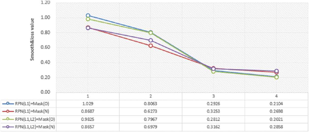
Comparison of gradient loss rate generated by region proposal network (RPN) and mask.

Table 2 shows the comparison of training parameters for the above four methods.

Method	RPN-Loss	Mask-Loss	AP	Elapsed Time
RPN (L1) + Mask (O)	Smooth = 1.029	Smooth = 0.2926	80.3%	37 m 45 s
	value = 0.8063	Value = 0.2104
RPN (L1) + Mask (N)	Smooth = 0.8687	Smooth = 0.3253	80.2%	39 m 59 s
	value = 0.6273	Value = 0.2698
RPN (L1, L2) + Mask (O)	Smooth = 0.9825	Smooth = 0.2812	81.1%	37 m 56 s
	value = 0.7967	Value = 0.2021
RPN (L1, L2) + Mask (N)	Smooth = 0.8657	Smooth = 0.3162	82.1%	41 m 03 s
	value = 0.6979	Value = 0.2858

RPN, region proposal network.

Table 2

Comparison of training parameters of mask RCNN model.

When the L1 and L2 norms are combined with the improved mask generation method, the accuracy precision (AP) value is the highest. The training time increases with the increase of the computational complexity of the model. In addition, in the training, we substitute the backbone network Resnet-101 with VGG19, Resnet-50, ResNeXt-50 and ResNeXt-101, each of which is combined with the improved Mask generation method respectively [22]. The comparison of AP and the training duration is shown in Table 3.

Backbone Networks	Method	AP (%)	Elapsed Time
Resnet-101	RPN (L1) + Mask (N)	80.2	39 m 59 s
	RPN (L1, L2) + Mask (N)	82.1	41 m 03 s
Resnet-50	RPN (L1) + Mask (N)	75.3	35 m 43 s
	RPN (L1, L2) + Mask (N)	77.7	35 m 40 s
VGG19	RPN (L1) + Mask (N)	73.2	33 m 21 s
	RPN (L1, L2) + Mask (N)	73.4	33 m 21 s
ResNeXt-50	RPN (L1) + Mask (N)	77.9	36 m 52 s
	RPN (L1, L2) + Mask (N)	78.4	37 m 19 s
ResNeXt-101	RPN (L1) + Mask (N)	83.7	43 m 05 s
	RPN (L1, L2) + Mask (N)	84.6	44 m 12 s

AP, accuracy precision; RPN, region proposal network.

Table 3

Comparison of training parameters for different basic backbone networks.

8.3. Test

With 1000 ship images as the test set, the test results of the improved method are compared with those of other methods. Through several groups of control experiments, the test model obtains the precision in accordance with Formula (13) and the recall in accordance with Formula (14). This index is used to measure the effect of the model on ship positioning.

(13)precision=TPTP+FP

(14)recall=TPTP+FN

Among them, TP represents the expected positive samples with the actual identification in line with the expectation, while FP represents the expected positive samples that the actual identification shows negative samples [23]. It is assumed that TP is the number of images that have accurately located the ship target, FP is the number of images that do not locate the ship target or just locate part of the ship targets and FN does not locate the ship target at all. We usually use the number of images whose test accuracy is lower than a certain low threshold value. The test results are shown in Table 4:

Method	Threshold Value	Precision (%)	Recall (%)
RPN (L1, L2) + Mask (N)	0.80	87	96
RPN (L1, L2) + Mask (N)	0.75	90	96
RPN (L1, L2) + Mask (O)	0.80	85	93
RPN (L1, L2) + Mask (O)	0.75	87	93

RPN, region proposal network.

Table 4

Test results.

When the threshold value is 0.80, the number of images whose recognition rate is greater than or equal to 0.80 is TP value, the number of images whose recognition rate is less than 0.80 but greater than or equal to 0.70 is FP value, and the number of images whose recognition rate is less than 0.70 is FN value.

When the threshold value is 0.75, the number of images whose recognition rate is greater than or equal to 0.75 is TP value, the number of images whose recognition rate is less than 0.75 but greater than or equal to 0.70 is FP value, and the number of images whose recognition rate is less than 0.70 is FN value.

It shows that the test precision and recall rate of the improved method are higher than those of the original method.

In this paper, Resnet-101, Resnet-50, VGG19 and ResNeXt-50, ResNeXt-101 are used to test the un-improved and improved mask generation models. Figure 11 shows the comparison of test precision of different models.

Figure 11

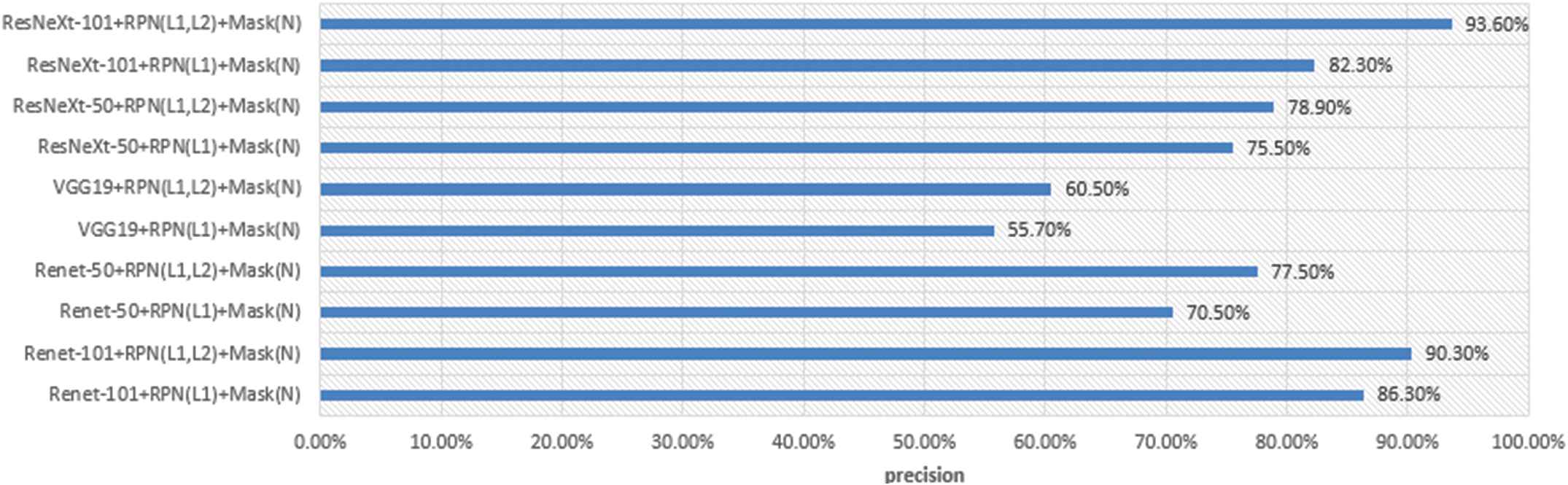
Comparison of test precision of different models.

As you can see from Figure 11, the model testing precision of ResNetXt-101 + RPN (L2) + Mask (N) is as high as 93.60%, which is 3.3% higher than that of ResNet-101 and 33.1% higher than that of VGG19. The data shows that the improvement of the basic backbone network is also a method to improve the model testing precision.

9. THE SOLUTION OF SHIP TARGET LOCATION

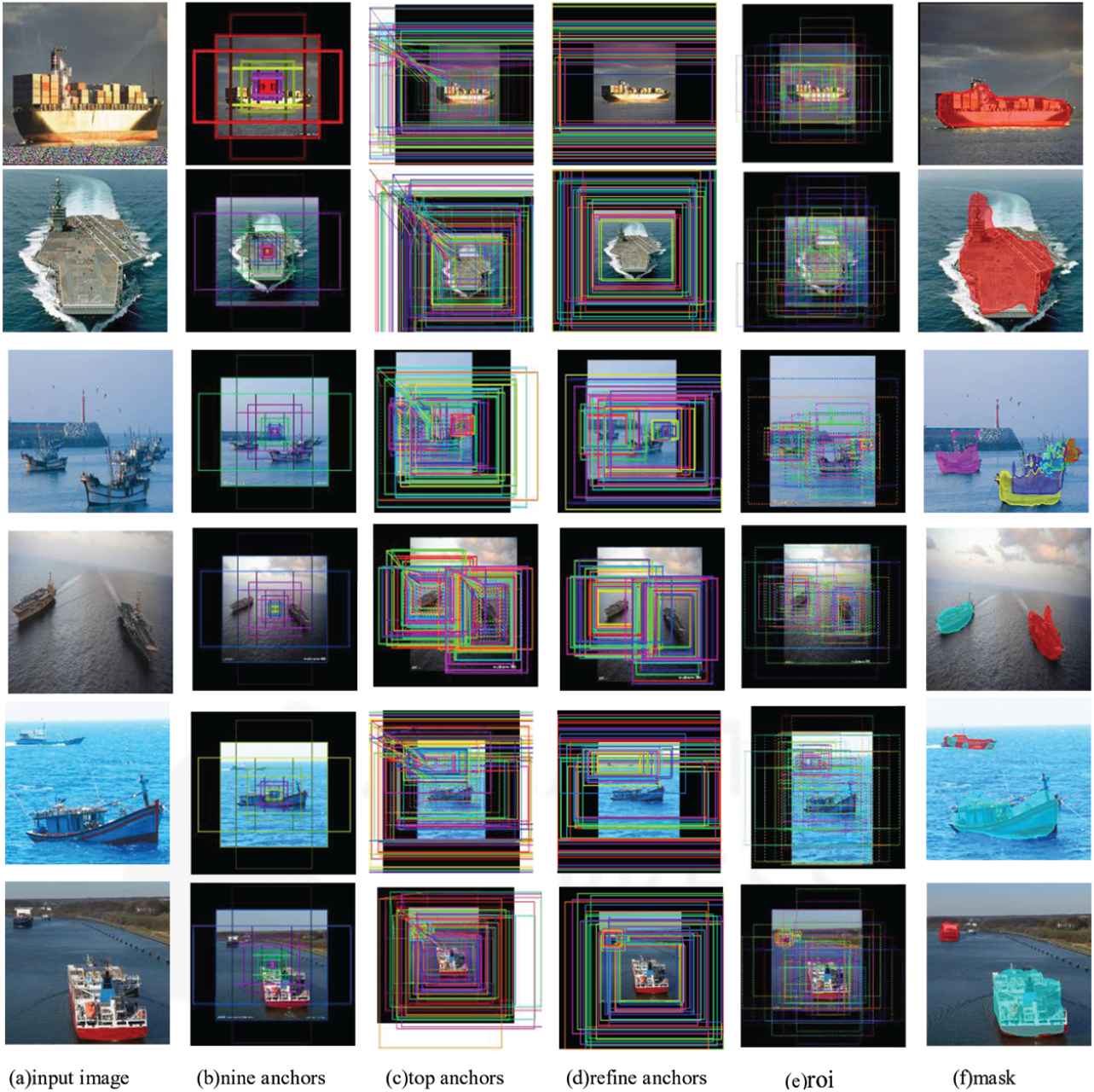
This paper defines the solution of ship target location through six processes:

(1) Image Input; (2) Anchor-Box Setting; (3) Top Anchor-Box Extraction; (4) Anchor-Box Selection and Optimization; (5) ROI Extraction; (6) Target Mask Generation (as shown in Figure 12). In this solution, three different ship types are tested, that is, ocean-going freighters, inshore fishing boats and large warships respectively. The test images are divided into three categories: close range, medium vision and prospect, as shown in Figure 12. Figure 12(a) displays the original image input with the size of 512*512, Figure 12(b) displays the nine anchor boxes of different colors from dark to light, Figure 12(c) displays the anchor box at the top of the extraction, and Figure 12(d) displays the remaining anchor box after cutting the edges of the image. Figure 12(e) displays the extracted ROI, and Figure 12(f) displays the mask generation for the target image. The testing result shows the processing effect of setting up RPN-Box, extracting ROI and generating mask in the un-improved and improved Mask RCNN network.

Figure 12

Solution of ship target location.

10. COMPARISON WITH OTHER METHODS

In this section, several models are compared and tested from the perspective of F1-score and run time. F1-score is used as matric for the network performance evaluation. We conduct the experiments to compare RCNN, Faster RCNN and Mask RCNN with the improved Mask RCNN. The results are shown in Table 5.

As shown in Table 5, the improved model has better F1-score performance. What's more, the performance of this model is 5.3% better than that of the Faster RCNN. This table also presents the running time of different models. As shown in Table 5, the running time of the proposed Mask RCNN is about 1 minute to 2 minutes slower than that of the existing technology. This shows that it will not cost too much to modify the Mask RCNN.

11. CONCLUSION

Aiming at detecting the target of offshore ships, this paper improves the RPN loss function of Mask RCNN and the target mask generation algorithm. In the process of distant hull detection, mask generation branches cannot ensure the precise segmentation for the instance, resulting in target loss or tiny interferences. We proposed an improved mask generation structure to solve these problems.

ResNet-101, ResNet-50, VGG19 and ResNeXt-50 and ResNeXt-101 are used to verify the precision and efficiency of ship target recognition. The test results show that the improved Mask RCNN model can detect and locate the target accurately, and the proposed Mask RCNN is more accurate than the existing ones. Although it will not cost a lot to modify the Mask RCNN, it still has the disadvantage that the mask generation cannot completely cover the edge of the target. In the following work, we will use the edge filtering algorithm combined with a larger sample base to further improve the precision of the model.

AUTHORS' CONTRIBUTIONS

Lin Shaodan contributed the central idea, analysed most of the data, and wrote the initial draft of the paper. The remaining authors contributed to refining the ideas, carrying out additional analyses and finalizing this paper.

ACKNOWLEDGMENTS

The authors would like to thank all the participants taken part in the experiments. This work was supported in part by the National Science Foundation of China (Grant No. 61841701) and the GuangDong Natural Science Foundation (Grant No. 2019B010137002) and Fujian Vocational College Intelligent Equipment Application Technology Collaborative Innovation Center Construction Project (Grant No. 2016-7) and the Science and Technology Project from Transportation Department of FuJian Province (Grant No. 201934).