
Efficient Time-Series Forecasting Using Neural Network and Opposition-Based Coral Reefs Optimization
- DOI
- 10.2991/ijcis.d.190930.003How to use a DOI?
- Keywords
- Meta-heuristics; Coral reefs optimization; Opposition-based learning; Neural networks; Time series forecasting; Nature-inspired algorithms; Distributed systems
- Abstract
In this paper, a novel algorithm called opposition-based coral reefs optimization (OCRO) is introduced. The algorithm is built as an improvement for coral reefs optimization (CRO) using opposition-based learning (OBL). For efficient modeling as the main part of this work, a novel time series forecasting model called OCRO-multi-layer neural network (MLNN) is proposed to explore hidden relationships in the non-linear time series data. The model thus combines OCRO with MLNN for data processing, which enables reducing the model complexity by faster convergence than the traditional back-propagation algorithm. For validation of the proposed model, three real-world datasets are used, including Internet traffic collected from a private internet service provider (ISP) with distributed centers in 11 European cities, WorldCup 98 contains request numbers to the server in football world cup season in 1998, and Google cluster log dataset gathered from its data center. Through the carried out experiments, we demonstrated that with both univariate and multivariate data, the proposed prediction model gains good performance in accuracy, run time and model stability aspects as compared with other modern learning techniques like recurrent neural network (RNN) and long short-term memory (LSTM). In addition, with used real datasets, we intend to concentrate on applying OCRO-MLNN to distributed systems in order to enable the proactive resource allocation capability for e-infrastructures (e.g. clouds services, Internet of Things systems, or blockchain networks).
- Copyright
- © 2019 The Authors. Published by Atlantis Press SARL.
- Open Access
- This is an open access article distributed under the CC BY-NC 4.0 license (http://creativecommons.org/licenses/by-nc/4.0/).
1. INTRODUCTION
Time series analytics and forecasting play an important role in many real-life areas, especially when the today's development of information technology and data explosion are blooming. The list of these areas gets longer (e.g. predicting human behaviors using collected data from wearable devices, flood forecasting based on historical water levels of rivers and springs, or monitoring financial stock exchange rates). In terms of time series forecasting, past observations are used to model relationships hidden in the data and to predict values in advance. In fact, this modeling way is very useful when there is a little knowledge about underlying data generation process. It is also useful when no adequate mathematical model is available to describe relationships between the predictor and other variables. Over the past several decades, the great effort has been devoted to the development and improvement of time series forecasting using various techniques.
The idea of time series forecasting for the value
To overcome the stationary assumption of statistical models, artificial neural network (ANN or NN) has been extensively studied and widely used also in time series forecasting [3]. The main advantage of ANN is the adaptability to nonlinear models i.e. the model is formulated based on the features detected from the data instead of specifying a concrete model template. This data-based approach is consistent with many empirical data sets, but there is no theoretical guideline to propose a generic data preparation process. Particularly in this direction, deep learning (DL), especially recurrent neural network (RNN) [4] are notable for sequence forecasting. This ability comes from RNN internal self-looped cells able to recognize sequence information. The most well-known RNN building block is long short-term memory (LSTM) [5], which also works well in processing long term time series data. However, DL techniques are compute-intensive that implies longer runtime.
Another way to deal with time series prediction goes through optimization using evolutionary bio-inspired algorithms [6], especially when most real-world optimizations are highly nonlinear and under various complex constraints. This kind of techniques trades in solution quality for runtime, by finding very good solutions, but not necessarily the optimal one within feasible time. Genetic algorithms (GAs) are a well-known evolutionary nature-inspired algorithm with a wide range of applications. Other algorithms can be listed here are particle swarm optimization (PSO), bacterial foraging optimization (BFO), coral reefs optimization (CRO) and many more.
Based on the state-of-the-art context, our main interest in this work is as follows:
If it is possible to develop a time series prediction model with simple structure, which can tackle the non-linear models and achieve comparable performance in the mean of accuracy and stability but with less runtime requirements in comparisons with other well-known models.
In order to test and evaluate the built model, optimizing operations of distributed applications is considered in this work. Nowadays, the number of distributed applications has been arising due to the extensive advances in distributed systems technology as well as the availability of data in various forms and formats. However, from the developer viewpoint, there are many difficult issues (e.g. consistency management, fault tolerance, security, location transparency, scalability, and performance) must be addressed to build complex distributed applications. The observation suggests that a serious effort to build an e-infrastructure for wide-area state sharing is highly recommended. Such infrastructure could help current applications scale better and significantly increase the rate at which complex distributed applications are deployed in the future. By applying time series data analytics techniques to e-infrastructures provided resources for distributed applications, the infrastructure can achieve the scalability as practical requirement mentioned above. This is also our foreseen of practical usage of this work as (but not limited to) an intelligent module for resource management for distributed/decentralized applications run on modern computing paradigms like clouds, Internet of Things systems, and blockchain networks.
The structure of this paper is organized as follows. Section 2 contains a survey with classification and analytics of existing studies to highlight the aim and contributions of our work. Section 3 and Section 4 present our proposed prediction model designs based on the opposite-base coral reefs optimization (OCRO) for multi-layer neural network (MLNN). In Section 5, we present experiments as well as evaluations for the proposed time series prediction model to prove its efficiency. Section 6 concludes and defines some of our future work directions.
2. RELATED WORK
2.1. Statistic Modeling
One of the most widely known and used time series prediction models is ARIMA [7]. The popularity of ARIMA is due to its statistical properties as well as effectiveness. It is flexible in representing different time series modeling such as standard AR, standard moving average (MA) or AR and MA combinations (ARMA) series. However, their main limitation is the linear form and they are appropriated for a time series that is stationary i.e. it's mean, variance, and autocorrelation should be approximately constant through time [8]. Besides, ARIMA models can not properly capture nonlinear patterns, so the approximation of these linear models to complex real-world problems is not enough to cover the variety characteristic like chaotic or nonlinear dynamic time series data [9].
2.2. Artificial Neural Networks
As stated in Section 1, ANNs have been applied to many areas for time series forecasting in order to overcome the limitations of linear models.
The work [10] employed a four-layered feed-forward neural network (FFNN), which is trained using back-propagation to make hourly predictions of electric load for a power system. Prediction accuracies with 1.07% error on weekdays and 1.80% on weekends were achieved that were superior of prediction accuracy over existing traditional time series forecasting methods. Authors of the work [11] presented an eight-step procedure to design a neural network forecasting model for financial and economic time series. In [12], the authors proposed the use of FFNN for inflows synthesis. FFNN offers a viable alternative also for multivariate modeling of water resources time series. The work [13] did not only employed ANNs for forecasting British pound and US dollar exchange rates but also evaluated the impact of input and hidden neurons number and data size on ANN model performance. The sensitivity analyses showed that the input affect effectiveness more than the hidden neurons and improved accuracies can be gained with larger sample size. In [14], the authors introduced an information gain technique used with machine learning for data mining to evaluate the predictive relationships of numerous financial and economic variables, and used FFNNs to forecast future values. The results show that trading strategies guided by the classification models generate higher risk-adjusted profits than the buy-and-hold strategy as well as those guided by the level-estimation based forecasts of NN and linear regression models. In [15], the authors designed three-layer FFNNs to predict the hourly solar radiation data, the result showed that FFNN outperforms linear prediction filters. Most of the studies reported above were simple applications of using traditional time series approaches and ANNs (FFNNs/MLNNs). In [14], the authors analyzed the drawbacks of MLNNs, which were usually not very stable since the training process may depend on the choice of a random start. Training is also computationally expensive in terms of the times used to determine the appropriate network structure. The degree of success, therefore, may fluctuate from one training pass to another.
The most well-known deep neural network (DNN) types for time series forecasting is RNN. The network type has cyclic connections in its structure, the activations from each time step are stored in the internal state of the network acts as temporal memory. This capability makes RNNs better suited for sequence modeling (i.e. time series prediction) and sequence labeling tasks. So, it has been more general models than FFNNs and has been widely used tool for the prediction of time series [16–20]. However, there are still two issues associated with the traditional RNN models in prediction problem, which are the number of time steps ahead has to be predetermined for most RNNs, and to achieve a better accuracy, finding the optimal time lag setting largely relies on the trial-and-error method. Previous studies [5] have confirmed that the traditional RNNs fail to capture the long temporal dependency for the input sequence, training the RNN with 510 time lags is proven difficult due to the vanishing gradient and exploding gradient problems. But RNNs are computationally and valuable approximation results more superior than FFNN prediction problems [21–23].
To address these drawbacks of RNNs, LSTM [5] was developed for forecast issue. Unlike traditional RNNs, LSTM is able to learn the time series with long time spans and automatically determine the optimal time lags for prediction. In the past two decades, LSTM has been successfully applied to robot control, speed recognition, handwriting recognition, human action recognition, transportation, etc. Especially, there are so many studies in time series prediction problem using LSTM such as [24–28]. Moreover, LSTM comes with a number of different variances such as gated recurrent unit (GRU), bidirectional LSTM, LSTM autoencoders [29,30], that promise further model quality improvements. However, the cost is often higher complexity, which requires a longer training.
Here also is suitable to mention that convolution neural network (CNN) is a strong candidate for sequence forecasting [31,32]. The combination of CNN and attention function brings the new architecture of temporal convolution nets (TCN), which outperforms RNN in several language-to-language translation benchmarks [33] at both speed and accuracy performances. In comparison with RNN, CNN structure is more natural to parallelize and this can be taken advantage to exploit accelerator supports.
Even DL and RNNs are considered as current state-of-the-art in the time series prediction field for a broad audience, it still has drawbacks. Concretely, DL requires a lot of data to train in order to gain more accurate, as well as a computational requirement because of the model complexity [34–36]. Particularly, RNNs are not parallelism-friendly due to their nested loop structures. However, the researches in this direction are interesting with high dynamics, that bring many advanced computing methods with promising results. It is also clear that the concern about performance from the speed viewpoint, as well as computational requirements still remains.
2.3. Neuro-Evolution
In “neuro-evolution” research community, GAs [37] are known as efficient search algorithms. Recently, GA-based research has been applied to NN models [38,39] in order to address computational cost, easy implement in hardware, and better accuracy. This direction is attracted to lots of researcher in many fields such as manufacturing process [40], stock markets [41], energy consumption [42], medical diagnosis [43], resource usage in cloud [44]. Unfortunately, recent research [45] identified some of the limitations in performance of GAs with problems have high epistasis targeting functions, the performance degradation is huge, and GA's early convergence lowers its performance and reduces its search capabilities.
In the term of combining NNs and optimization algorithms, swarm intelligent (SI) optimization motivated by social behavior in the biological system also has attracted many researchers. PSO was stimulated by swarm behavior of bird flocking or fish schooling has been used in several real-life area [46]. BFO, which is an evolutionary computing technique inspired based on the principle of bacterial movement like tumbling, swimming, or repositioning to food-seeking [47]. An improved version of BFO is Adaptive BFO with life-cycle and social learning (ABFO) was developed and presented in [48]. It has been tested on several sets of benchmark functions with multiple dimensions and used in distributed systems like cloud computing [49]. In a recent development, a bunch of meta-heuristics swarm-based intelligence algorithms were developed, which can be used to optimized NNs. The list contains Moth-flame optimization algorithm [50], Whale optimization algorithm [51], Salp Swarm Algorithm [52], Grasshopper optimization algorithm [53], Harris Hawks optimization [54], Butterfly optimization algorithm [55], Sailfish optimization algorithm [56], and many more.
2.4. Coral Reefs Optimization
This technique also belongs to SI optimization algorithms motivated by social behavior in the biological systems like PSO, BFO, and other swarm-based heuristics. It is proposed in [57] tackling optimization problems by modeling and simulating corals reproduction and formation. A lot of applications have been carried out in many areas such as energy prediction [58,59], sensor networks [60], and cloud resource allocation [61].
The original CRO algorithm simulates a coral reef, where different corals grow and reproduce in coral colonies, fighting by choking out other corals for space in the reef. This fight for space produces a robust meta-heuristic algorithm powerful for solving hard optimization problems. According to [62], the exploitive power of CRO is controlled by broadcast spawning, which carries out most of the global searching and brooding that could help jump out of the local optima. In this approach, a fraction of healthy reef can duplicate itself and larvae setting process controls local searching by a simulated annealing (SA) alike process as exploitive power (mostly) executed in the budding process.
Like other meta-heuristic algorithms, CRO has also the problem with local optimums. The diversity of corals in a reef quickly decreases after a certain number of iterations, which causes stuck in a local area and it is hard to jump out of it. In order to improve the CRO's searching power, we propose an improvement that combines the technique with a well-regarded mathematical concept called opposition-based learning (OBL) initially proposed in [63]. OBL can attain the opposite locations for candidate solutions for a given task. The new location can provide a new chance to become aware of a neighboring point to the best position. In this work, we call our new improvement under the short-name OCRO, which stands for OBL in combination with CRO.
2.5. Contributions of the Work
Currently based on our knowledge, there is no study that applies the CRO to MLNN and OCRO to MLNN. In comparison with above-mentioned works, the main differences and contributions of our work are as follows.
Proposing a new improvement called opposition-based coral reefs optimization (OCRO), which improves the original CRO algorithm using OBL. OCRO aims to improve searching power and jumping out from the local minimum of the meta-heuristic CRO.
From the theoretical viewpoint, when the combination of CRO and OBL is property applied to MLNN, it improves the drawbacks of gradient descent algorithm, enables fast convergence to optimal values as well as reducing computational cost as the whole.
Proposing the new time series forecasting model called OCRO-MLNN, which is designed based on MLNN variance with OCRO algorithm to train the forecasting model instead of back-propagation.
Carrying out comparisons among the novel proposed prediction model with five well-known ones such as MLNN, GA-MLNN, CRO-MLNN, RNN, and LSTM for time series forecast.
Evaluating and proving the effectiveness of OCRO-MLNN as compared with others using three kinds of real-world datasets (i.e. above-mentioned European (EU) traffic, world cup (WC), and Google trace). The gained outcomes show that our prediction model OCRO-MLNN provide good performance in predictive accuracy, model stability, as well as runtime.
3. OPPOSITION-BASED CORAL REEFS OPTIMIZATION
3.1. Coral Reefs Optimization
As mentioned above, CRO is an optimization algorithm (bio-)inspired by behaviors of corals reproduction and reef formation. It was originally introduced in [57]. The skeleton of the original CRO is summarized in Algorithm 1 that includes two main below-described parts.
Algorithm 1: CRO algorithm
Initialization
Create a
while not stopCriteria() do:
Broadcast spawning
A fraction of
Brooding
The rest of
Larvae setting
Asexual reproduction
Depredation in polyp phase
Return the best solution.
Part 1: Initialization of CRO parameters.
The main control parameters of CRO are as follows: a coral reef consists of an
Part 2: Reef information.
Broadcast Spawning (external sexual reproduction):
Select uniformly at random a fraction of existing corals (
Broadcast spawner couples will produce a coral larva by sexual crossover. These couple selection can be done uniformly at random or by resorting to any fitness proportionate selection approach (e.g. roulette wheel). Note that once two corals have been selected to be the parents of larvae, they are not selected anymore in the broadcast spawning phase.
Brooding (internal sexual reproduction): As described in Step (1), the fraction
Larvae setting: When all the larvae are formed by the broadcast spawning or by brooding, the process of setting and growing in the reef will be performed. Firstly, the health function of each larva is evaluated. Then, each larva will randomly settle down in the
Asexual reproduction (budding or fragmentation): According to the values of health function, existing corals are rearranged in the reef. A proportion of
Depredation in polyp phase: In the process of reef formulation, corals also die, and their space is freed up for newly generated corals. The depredation operator is applied with a very small probability
3.2. Opposition-based Coral Reefs Optimization
According to [62], the ability to exploit of CRO is controlled by broadcast spawning. This carries out most of the global searching and brooding, which helps to jump out of the local optimal. As for exploitive power, mostly executed by building process, where a fraction of healthy reef can duplicate itself and larvae setting process controls local searching by SA like process. Like other meta-heuristic algorithms, CRO is also faced with trapping in local optimal. The diversity of corals in reef quickly decrease after several iterations, causes the algorithm stuck in the local area and hard to jump out of it.
In order to improve the CRO's searching power, we propose an improvement (called OCRO in short name) that combine it with OBL [63] mathematical concept well-known in reinforcement learning, ANNs, and fuzzy systems. All code and related materials are stored as open-source at [64]. OBL indicates that for finding the unknown optimal solution, searching both a random direction and its opposite simultaneously gives a higher chance to find the promising regions and to enhance the algorithm performance [65]. Our improvement for CRO based on OBL is built as follows.
OBL attains opposite locations for candidate solutions for a given task. The new location can provide a new chance to become aware of a neighboring point to the best position.
OBL is applied in the CRO depredation phase instead of removing the worst health fraction of reef. We calculate the potential of the oppositional solution
Oppositional coral is generated by Equation (1):
| is the position of opposite coral |
|
| is the lower bound of the search space, | |
| is the upper bound of the search space, | |
| is the best coral (the best solution), | |
| is a random vector with elements inside range |
The improvement of depredation step is formed through Algorithm 2.
Algorithm 2: OCRO - Improvement of CRO depredation step
Randomly select a number of worse health coral
for C in DeCorals do
if
else
Depredate C and free space in reef
To prevent premature convergence to a local optimum, in our improvement, we restart the search process when the best solution is not improved after several generations based on [66]. When the reef is restarted, the best coral is maintained (elitism criterion) and the rest of corals are randomly initialized. The results of our new proposed OCRO algorithm, which is the combination and improvement of CRO with OBL, are optimistic as presented and discussed below in Section 5.2.
4. NONLINEAR TIME SERIES FORECASTING USING NEURAL NETWORK AND OPTIMIZATION
4.1. Time-Series Modeling Using Neural Network
ANNs (in general) and MLNNs (in particular) are flexible computing frameworks for modeling a broad range of nonlinear problems. In comparison with other nonlinear models, MLNN advantages are their ability as universal approximators with a large class of functions producing high accuracy degree. This advantage comes not only from the fact that NN model is based on data characteristics (hence, no prior assumption of the model form is required), but also the ability to process information from the data in parallel. MLNNs are often used for pattern classification and recognition. Recently, FFNNs with single hidden layer are also widely used as time series forecaster [3]. The model includes three layers which are input, hidden, and output layer as represented by Figure 1 (left side). Each of them has simple processing units connected by acyclic links. The relationship between outputs (
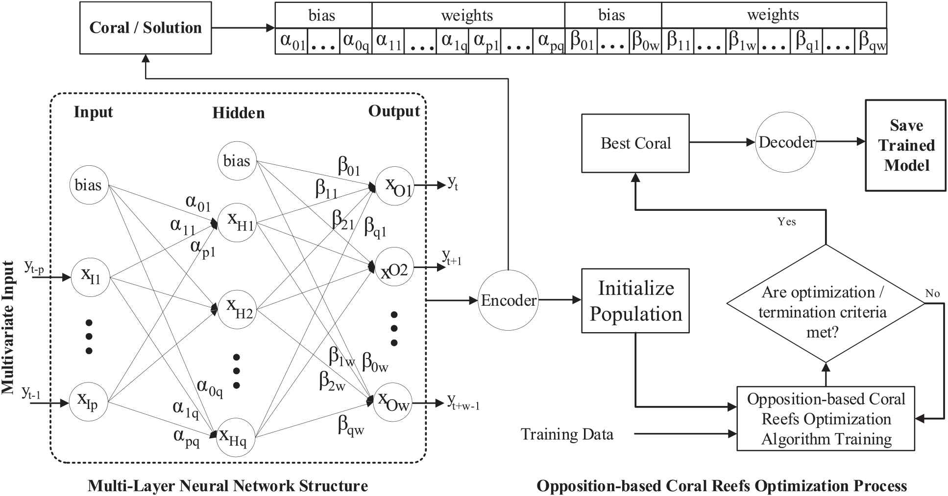
Opposition-based coral reefs optimization (OCRO)-multi-layer neural network (MLNN) training process.
| is connection weight for |
|
| is connection bias for |
|
| is the number of input nodes, | |
| is the number of hidden nodes, | |
| is the number of output nodes, | |
| is activation function of input |
In the past, logistic functions were often used as activation function but recently exponential linear unit (ELU) presented by Equation (3) (general formula) gains more interests (
The choice of
The same situation as mentioned above also occurs when choosing the number of lagged observations
In time series forecasting,
Once the structure (
4.2. OCRO-MLNN Forecasting Model
As presented before, our prediction model uses OCRO algorithm to optimize the selection of weights and biases of hidden and output layers. Thus, we focus on improving the overall performances, including accuracy, speed of convergence and stability of the MLNN network instead of using the back-propagation technique. The number of variables estimated by OCRO is as follows.
Range of individual variables is set to
The learning process of OCRO-MLNN is illustrated by Figure 1. To obtain the multivariate input, raw data is preprocessed by the following steps.
Firstly, a time series data is scaled into the range of
Secondly, time series data is transformed to supervised data using the sliding method with window width
Finally, all metric types are grouped into multivariate input. Encoder and decoder are two important components in Figure 1. In which, encoder encodes NN weights and biases into our domain solution (i.e. coral presented as real-value vector). Decoder decodes corals back into NN weights and biases.
In order to avoid long training time, a termination criterion is designed for earlier-stopping after the number of epochs (training cycles) is predefined or after the achievement of error goal.
Algorithm 3 describes the MLNN operation with OCRO. The parameters are shown in Table 1.
| Name | Description |
|---|---|
| Maximum number of generations | |
| Number of square grids in reef | |
| The rate between free/occupied squares in reef at the beginning of this algorithm | |
| The fraction of broadcast spawners with respect to the overall amount of existing corals | |
| The fraction of corals that will reproduce by brooding | |
| A fraction of reef that will duplicates itself | |
| A fraction of worse health corals will be depredated | |
| Number of attempts for a larva to set in the reef | |
| Number of iterations before restarting the algorithm |
Opposition-based coral reefs optimization (OCRO) parameters.
5. EXPERIMENTS AND EVALUATIONS
5.1. Evaluation Approach
Under assumption of the same datasets, settings, and testing environment, two experiment groups are carried out to evaluate the proposed OCRO-MLNN model, covering:
Evaluating the proposed model on both univariate and multivariate data of different datasets.
For each test, prediction accuracy, run-time, and model stability among various NN models are compared with our OCRO-MLNN model.
Algorithm 3: OCRO-MLNN forecasting model
Input:
Output:
1: Initializing reef space includes
2: for i = 0 to
3:
4:
5:
6: for
7: Crossover
8: for
9: Mutation
10: for larva in larvaes do
11: for j = 0 to k do
12: square
13: if square is empty or
14: square
15: break
16:
17:
18: Run step 11 to 16 (Larvaes setting) for
19: for
20:
21: if
22: Replace
23: else
24: Free space at
25: Find the best current coral
26: if
27:
28: if
29: Restart searching, keep
30: Return
Other NN models used for comparison include traditional MLNN and its variances with optimization techniques such as GA-MLNN, PSO-MLNN, ABFO-MLNN, CRO-MLNN, traditional RNN and the state-of-the-art LSTM.
5.1.1. Datasets
Univariate data. Univariate data used in our experiments are two real and well-known datasets, covering:
“Internet traffic data (in megabytes)” [68] collected from a private internet service provider (ISP) with distributed centers in 11 European cities (in short from here EU dataset). The dataset corresponds to a transatlantic link and was collected from June 7th to 11:17 hours on July 31st, 2005 in five minutes intervals.
The second dataset (called WorldCup98, in short from here WC dataset) contains request numbers (in thousands) to servers in world-cup season between April 30th, 1998 and July 26th, 1998. The dataset is processed into five minutes intervals in our work.
Multivariate data. Multivariate data used in our experiments are gathered by Google from their production data center clusters (called Google trace dataset, in short from here Google dataset). The log records come from approximately 12000 servers for one month [69] and [70]. Based on our prior analysis presented in [44], we select both resource usages, which are central processing unit (CPU) and memory metric as multivariate inputs for our proposed models. The dataset also was further processed into five minutes intervals in the experiments. Visualization of both data type is illustrated in Figure 2.
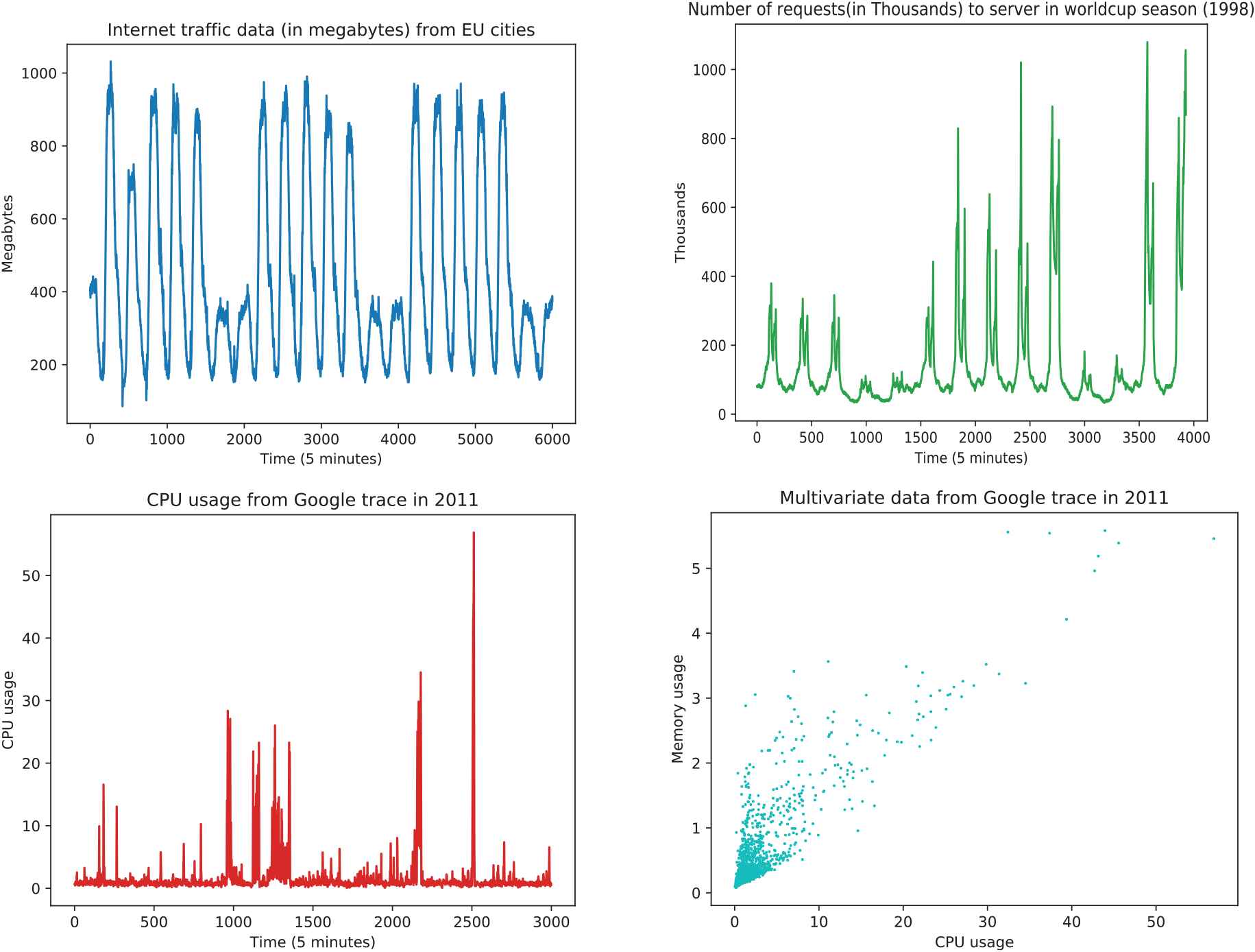
Dataset visualizations: univariate data (upper row) and multivariate data (lower row).
Due to the characteristics of time series data, which is ordered time-dependency sequence, hold-out validation with 70:15:15 ratio is used as the splitting parameter for training/validation/testing datasets. This splitting approach is designed also as adjustable time slider frame for cross-validation for potential time-growing datasets [71,72].
5.1.2. Measurement methods
Accuracy. In our work, root mean square error (RMSE) (Eq. 5) is used mainly to evaluate error between predicted and ground true value. It is also employed as the fitness function in GA, PSO, ABFO, and as the health function in CRO and OCRO. However, for objectiveness, other metrics such as Coefficient of Determination (
Runtime. The proposed model OCRO-MLNN is also compared with other models in runtime performance-wise (speed) aspect. Currently, RNN and particularly LSTM are state-of-the-art for time series prediction models. The fact is their complicated structure and training runtime often is long. Hence, it is desired to have a model with at least comparable good prediction performance but less expensive on computational requirement. The runtime comparison in our experiments is done according to three factors:
Because each model has different epoch configuration,
5.1.3. Settings parameters for algorithms and models
As described above, OCRO-MLNN is validated against other modes such as MLNN, GA-MLNN, PSO-MLNN, ABFO-MLNN, CRO-MLNN, RNN, and LSTM.
MLNN part in the all models listed above is configured with the same structure configuration with three layers: input, hidden, and output layer. The architecture is similar to typical topology of one RNN/LSTM block [25].
Input size
In RNN and LSTM models, NN is composed from one input layer, one RNN/LSTM block and one output layer with similar parameter settings. Activation function used in the models is ELU as described above in Section 4.
To be fair in all test, the population size
Besides above-described common specifications for fairness testing, the following settings are applied to algorithms for their best tested performance.
For GA, probability of two individuals exchanging crossovers
For PSO, based on [73], inertia factor
For ABFO, according to our prior experiment [49], swimming length is set
For CRO, based on [57], initial free/occupied square (
For OCRO, most of parameters are set similar to CRO except broadcast spawning fraction
- –
For
- –
Our proposed
- –
- –
5.2. Experiment Results
5.2.1. Univariate data
Prediction accuracy. Table 2 describes obtained experiment results with above-mentioned models on two datasets. The overall evaluation is as follows.
In general, the accuracy of MLNN and ABFO-MLNN models did not bring performance well as the comparison with the rest.
With the EU dataset, our proposed OCRO-MLNN performances has the best with (RMSE, MAE) = (15.535, 11.058) and (15.381, 10.918) for
LSTM get the best results with index of
With the WC dataset, for all four metrics
| Data | Model | RMSE |
MAE |
MAPE |
SMAPE |
||||||
|---|---|---|---|---|---|---|---|---|---|---|---|
| EU | MLNN | 0.9931 | 0.9936 | 20.484 | 19.599 | 15.826 | 15.359 | 4.357 | 4.362 | 4.268 | 4.260 |
| GA-MLNN | 0.9953 | 0.9946 | 15.807 | 16.952 | 11.452 | 12.225 | 3.078 | 3.267 | 3.062 | 3.281 | |
| ABFO-MLNN | 0.9942 | 0.9917 | 17.552 | 20.959 | 13.338 | 15.536 | 3.921 | 4.216 | 3.851 | 4.308 | |
| PSO-MLNN | 0.9954 | 0.9955 | 15.712 | 15.474 | 11.347 | 11.139 | 3.072 | 3.002 | 3.061 | 3.002 | |
| CRO-MLNN | 0.9954 | 0.9950 | 15.586 | 16.364 | 11.100 | 11.840 | 2.939 | 3.216 | 2.940 | 3.207 | |
| RNN | 0.9956 | 0.9958 | 16.263 | 16.866 | 11.624 | 11.320 | 2.954 | 2.894 | 2.977 | 2.911 | |
| LSTM | 0.9958 | 0.9959 | 15.857 | 15.786 | 11.358 | 11.497 | 2.899 | 2.973 | 2.902 | 2.956 | |
| OCRO-MLNN | 0.9955 | 0.9956 | 15.535 | 15.381 | 11.058 | 10.918 | 2.933 | 2.903 | 2.930 | 2.900 | |
| WC | MLNN | 0.9805 | 0.9565 | 29.562 | 44.164 | 13.287 | 20.083 | 5.708 | 8.892 | 5.884 | 8.737 |
| GA-MLNN | 0.9912 | 0.9834 | 19.876 | 27.253 | 8.173 | 10.758 | 4.806 | 4.882 | 4.655 | 4.822 | |
| ABFO-MLNN | 0.9800 | 0.9763 | 27.487 | 29.971 | 10.223 | 10.264 | 4.555 | 4.690 | 4.588 | 4.675 | |
| PSO-MLNN | 0.9736 | 0.9918 | 34.385 | 19.176 | 12.244 | 8.447 | 4.823 | 4.633 | 4.900 | 4.637 | |
| CRO-MLNN | 0.9915 | 0.9910 | 19.475 | 20.111 | 8.535 | 8.603 | 4.439 | 4.367 | 4.429 | 4.411 | |
| RNN | 0.9780 | 0.9854 | 28.833 | 23.468 | 11.440 | 10.442 | 4.644 | 4.388 | 4.677 | 4.347 | |
| LSTM | 0.9880 | 0.9892 | 21.300 | 20.195 | 8.776 | 8.519 | 4.455 | 4.319 | 4.435 | 4.328 | |
| OCRO-MLNN | 0.9856 | 0.9937 | 25.388 | 16.808 | 10.128 | 7.290 | 4.383 | 4.340 | 4.348 | 4.320 | |
RMSE, MAPE and
Table 2 shows that OCRO-MLNN not only improves the original CRO-MLNN but also gets better accuracy as compared with LSTM and others. In which the bold numbers indicate the best gained test results of OCRO-MLNN with different measurements. Figure 3 and Figure 4 express the prediction results to illustrate the gained data.
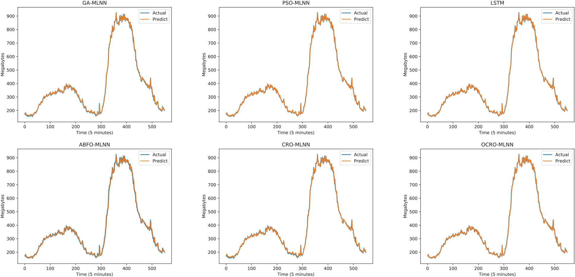
Comparison of opposition-based coral reefs optimization (OCRO)-multi-layer neural network (MLNN) prediction with other models (sliding window = 2; EU dataset).
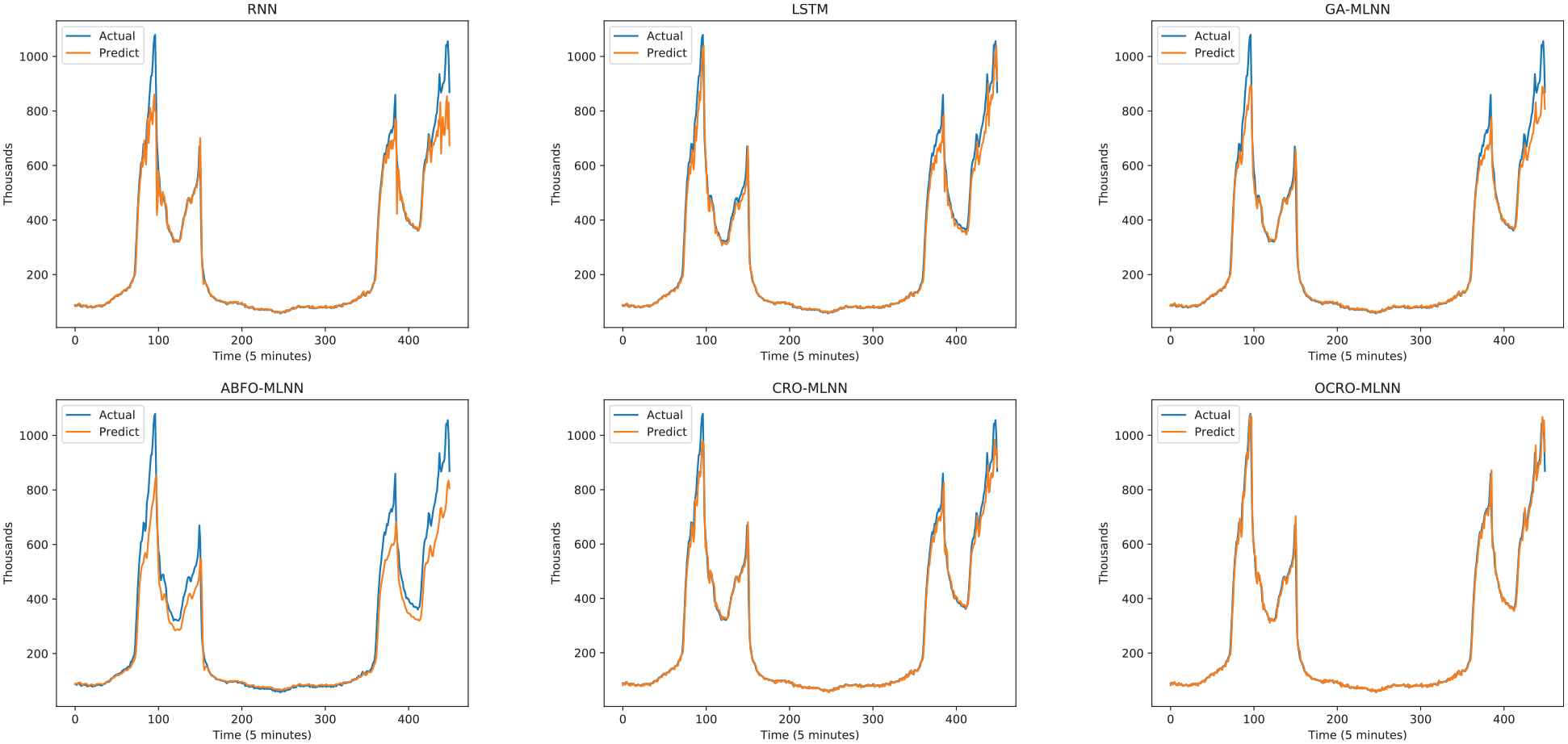
Comparison of opposition-based coral reefs optimization (OCRO)-multi-layer neural network (MLNN) prediction with other models (sliding window = 5; world cup (WC) dataset).
Runtime comparison. Table 3 shows runtime measurements of experiments. Note that epoch settings are described in detail in 5.1.3. There are some observations, which can be made as follows.
RNN and LSTM have a quite high runtime. For instance, with
Traditional MLNN's have significant small training time per epoch in comparison with others model. The disadvantage of MLNNs is that it converges slowly, requiring many epoch to train. Therefore the training time will be more and cause a slow effect on overall.
OCRO-MLNN and CRO-MLNN provide good runtime performance to complete all work with encouraging results. The reason is their short runtime per epoch and quick convergence.
- –
EU traffic dataset: OCRO-MLNN's runtime
- –
WC dataset: OCRO-MLNN's runtime
- –
| Data | Model | ||||||
|---|---|---|---|---|---|---|---|
| EU | MLNN | 0.1338 | 0.1692 | 669.42 | 0.1384 | 0.1273 | 692.22 |
| GA-MLNN | 0.9397 | 0.0011 | 657.77 | 0.9202 | 0.0014 | 644.13 | |
| ABFO-MLNN | 0.9487 | 0.0011 | 664.11 | 0.9772 | 0.1112 | 684.04 | |
| PSO-MLNN | 0.9182 | 0.0015 | 642.73 | 0.9089 | 0.0014 | 636.25 | |
| CRO-MLNN | 0.5091 | 0.0014 | 356.36 | 0.5145 | 0.0014 | 360.18 | |
| RNN | 2.1575 | 0.5054 | 2158.05 | 3.8974 | 0.7084 | 3898.13 | |
| LSTM | 1.8913 | 0.4376 | 1891.72 | 3.8137 | 0.6273 | 3814.30 | |
| OCRO-MLNN | 0.5054 | 0.0010 | 353.79 | 0.4925 | 0.0012 | 344.78 | |
| WC | MLNN | 0.0895 | 0.2358 | 448.04 | 0.0919 | 0.2466 | 459.92 |
| GA-MLNN | 0.6449 | 0.0012 | 451.43 | 0.6580 | 0.0018 | 460.58 | |
| ABFO-MLNN | 0.6701 | 0.0009 | 469.10 | 0.6899 | 0.0008 | 482.97 | |
| PSO-MLNN | 0.6241 | 0.0008 | 436.86 | 0.6382 | 0.0008 | 446.76 | |
| CRO-MLNN | 0.3496 | 0.0008 | 244.74 | 0.3665 | 0.0009 | 256.59 | |
| RNN | 0.9773 | 1.1465 | 978.41 | 1.9293 | 1.2888 | 1930.61 | |
| LSTM | 0.8450 | 0.8934 | 845.93 | 1.9264 | 1.2296 | 1927.63 | |
| OCRO-MLNN | 0.3462 | 0.0008 | 242.33 | 0.3537 | 0.0012 | 242.33 | |
Runtime comparison (sliding window
Model stability. Table 4 presents the comparison of OCRO-MLNN with other models on RMSE (average statistics after 15 run times). There are several short evaluations and remarks as follows.
MLNN model obtains the worst results with very high standard deviation (
The proposed OCRO-MLNN obtains in experiments RMSE values in range from 16.6236 to 24.7484,
ABFO-MLNN and RNN model also gain quite bad results in stability when comparing to LSTM, CRO-MLNN, and OCRO-MLNN. For more detail, with the EU dataset, sliding window
| Data | Model | k = 2 |
k = 5 |
||||||||
|---|---|---|---|---|---|---|---|---|---|---|---|
| EU | MLNN | 15.8611 | 30.4864 | 19.2223 | 4.1926 | 0.2181 | 16.2603 | 31.9792 | 25.6531 | 4.0866 | 0.1593 |
| RNN | 16.0049 | 20.984 | 17.7525 | 1.8485 | 0.1041 | 16.0111 | 21.908 | 17.9194 | 2.2523 | 0.1257 | |
| LSTM | 15.585 | 16.5124 | 16.0292 | 0.2314 | 0.0144 | 15.7024 | 18.6302 | 16.4398 | 0.8462 | 0.0515 | |
| GA-MLNN | 15.5587 | 19.7204 | 17.152 | 1.3099 | 0.0764 | 15.6322 | 20.7341 | 17.5186 | 1.3395 | 0.0765 | |
| PSO-MLNN | 15.5566 | 16.2584 | 15.7078 | 0.1961 | 0.0125 | 15.3195 | 17.8479 | 16.1036 | 0.7924 | 0.0492 | |
| ABFO-MLNN | 15.9053 | 19.5867 | 17.1062 | 1.1966 | 0.07 | 16.4715 | 25.7909 | 21.5049 | 2.6538 | 0.1234 | |
| CRO-MLNN | 15.5244 | 16.4715 | 15.822 | 0.278 | 0.0176 | 15.5357 | 17.8479 | 16.1219 | 0.5448 | 0.0338 | |
| OCRO-MLNN | 15.5151 | 15.5667 | 15.5441 | 0.0142 | 0.0009 | 15.3013 | 15.996 | 15.5697 | 0.2194 | 0.0141 | |
| WC | MLNN | 18.771 | 67.5236 | 33.0351 | 12.6737 | 0.3836 | 19.5462 | 61.4193 | 38.9827 | 12.5872 | 0.3229 |
| RNN | 20.488 | 35.0887 | 27.4246 | 3.8517 | 0.1404 | 18.0851 | 30.6916 | 23.1305 | 3.3629 | 0.1454 | |
| LSTM | 17.6447 | 31.5707 | 24.6919 | 4.5824 | 0.1856 | 18.035 | 27.9699 | 22.1468 | 3.5013 | 0.1581 | |
| GA-MLNN | 18.0851 | 30.6916 | 22.7368 | 3.2264 | 0.1419 | 18.6348 | 35.3217 | 23.3347 | 5.1492 | 0.2207 | |
| PSO-MLNN | 16.7875 | 34.5682 | 26.4276 | 5.2702 | 0.1994 | 16.8053 | 29.5606 | 20.3284 | 3.8017 | 0.187 | |
| ABFO-MLNN | 16.6236 | 38.7891 | 23.2257 | 6.8395 | 0.2945 | 19.2615 | 41.0411 | 28.1293 | 6.8486 | 0.2435 | |
| CRO-MLNN | 16.7806 | 28.7189 | 21.4259 | 3.4962 | 0.1632 | 17.5025 | 33.8349 | 23.4025 | 4.5302 | 0.1936 | |
| OCRO-MLNN | 16.6236 | 24.7484 | 20.0339 | 1.8681 | 0.0932 | 16.9945 | 27.0219 | 20.5392 | 2.5978 | 0.1265 | |
RMSE comparison (average of 15 times; univariate dataset)
Figure 9 visualizes RMSE range of 15 run times averages with tested models using box-and-whisker plots. While the intermittent lines in the middle of boxes represent the mean values, the upper and lower boundaries of the boxes represent the upper and lower quantiles of the distributions.
5.2.2. Multivariate data
Prediction accuracy. Table 5 shows the gained experiments results with all tested models on multivariate data in the aspect of accuracy. The evaluations can be made as follows.
| Data | Model | RMSE |
MAE |
MAPE |
SMAPE |
||||||
|---|---|---|---|---|---|---|---|---|---|---|---|
| CPU | MLNN | 0.0828 | 0.0742 | 0.529 | 0.504 | 0.363 | 0.344 | 36.089 | 39.629 | 42.218 | 34.075 |
| GA-MLNN | 0.1012 | 0.1339 | 0.465 | 0.445 | 0.302 | 0.316 | 36.822 | 36.193 | 31.347 | 29.858 | |
| ABFO-MLNN | 0. 0861 | 0.0779 | 0.494 | 0.500 | 0.324 | 0.315 | 39.914 | 35.130 | 31.839 | 31.646 | |
| PSO-MLNN | 0.1312 | 0.1370 | 0.453 | 0.452 | 0.307 | 0.303 | 36.550 | 35.859 | 30.705 | 30.393 | |
| CRO-MLNN | 0.1461 | 0.1523 | 0.449 | 0.448 | 0.304 | 0.300 | 36.461 | 35.687 | 30.512 | 30.251 | |
| RNN | 0.1332 | 0.1568 | 0.485 | 0.478 | 0.315 | 0.305 | 38.648 | 35.841 | 31.280 | 30.558 | |
| LSTM | 0.1664 | 0.1839 | 0.476 | 0.452 | 0.302 | 0.294 | 36.385 | 35.297 | 30.227 | 31.287 | |
| OCRO-MLNN | 0.1812 | 0.1922 | 0.440 | 0.437 | 0.294 | 0.298 | 35.403 | 35.523 | 29.710 | 29.977 | |
| RAM | MLNN | 0.5411 | 0.4652 | 0.038 | 0.068 | 0.027 | 0.058 | 12.008 | 27.195 | 11.547 | 23.307 |
| GA-MLNN | 0.6663 | 0.6426 | 0.032 | 0.033 | 0.021 | 0.021 | 9.923 | 9.613 | 9.745 | 9.514 | |
| ABFO-MLNN | 0.6860 | 0.5241 | 0.033 | 0.043 | 0.022 | 0.034 | 9.621 | 15.962 | 9.535 | 14.616 | |
| PSO-MLNN | 0.6758 | 0.6560 | 0.032 | 0.033 | 0.020 | 0.021 | 8.883 | 9.357 | 8.880 | 9.317 | |
| CRO-MLNN | 0.6572 | 0.6455 | 0.033 | 0.033 | 0.021 | 0.022 | 9.358 | 9.772 | 9.365 | 9.811 | |
| RNN | 0.6927 | 0.6684 | 0.034 | 0.034 | 0.019 | 0.022 | 9.521 | 9.756 | 9.577 | 9.974 | |
| LSTM | 0.7069 | 0.6924 | 0.033 | 0.034 | 0.021 | 0.018 | 9.203 | 9.243 | 9.135 | 9.329 | |
| OCRO-MLNN | 0.7092 | 0.6875 | 0.031 | 0.032 | 0.018 | 0.021 | 8.792 | 9.091 | 8.789 | 9.165 | |
RMSE, MAPE and
MLNN model achieves the worst results in this test. The low accuracy problem of this model caused by gradient descent when searching for an optimal solution in a complex dimension.
OCRO-MLNN model obtains the best results indicating high accuracies in both multivariates tested data types (shown by Table 5).
In comparison OCRO-MLNN with LSTM, both models gain the top results alternately with small difference. Concretely, the outcomes are as follows.
- –
For CPU metric: sliding window
- –
For random-access memory (RAM) metric: sliding window
- –
These experiments presented above indicate that with multivariate data, our OCRO-MLNN model performs well as compared with others. Figures 5 and 6 are used to show predictive results of different models gained via the experiments.
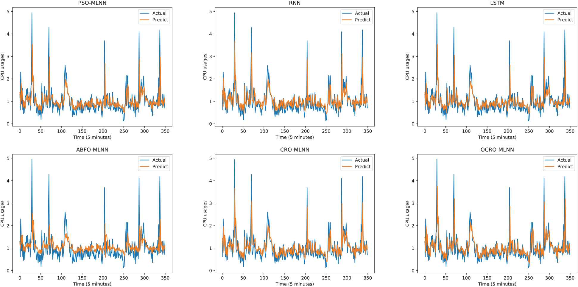
Comparison of opposition-based coral reefs optimization (OCRO)-multi-layer neural network (MLNN) prediction with other models (sliding window = 2; multivariate data - CPU).
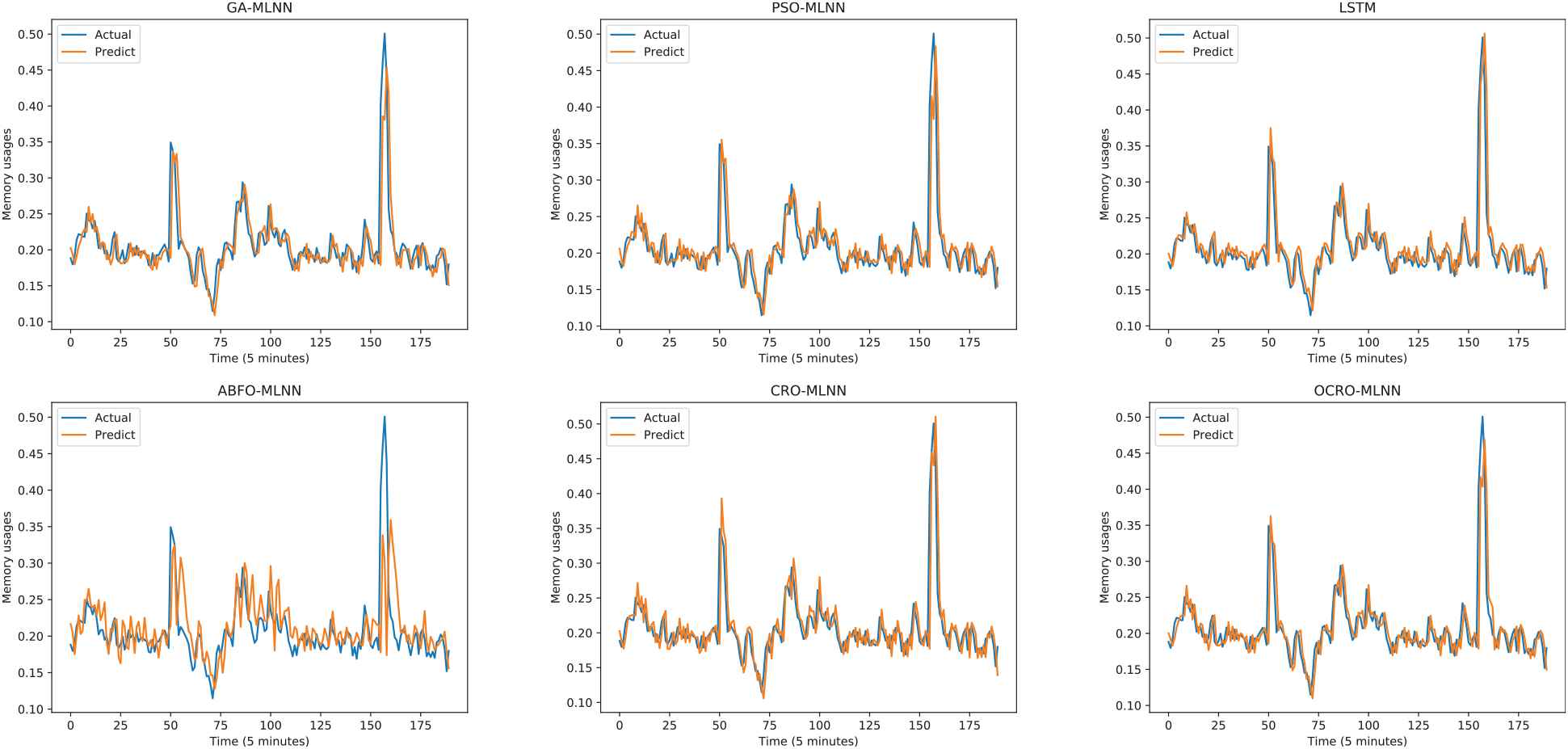
Comparison of opposition-based coral reefs optimization (OCRO)-multi-layer neural network (MLNN) prediction with other models (sliding window = 5; multivariate data - RAM).
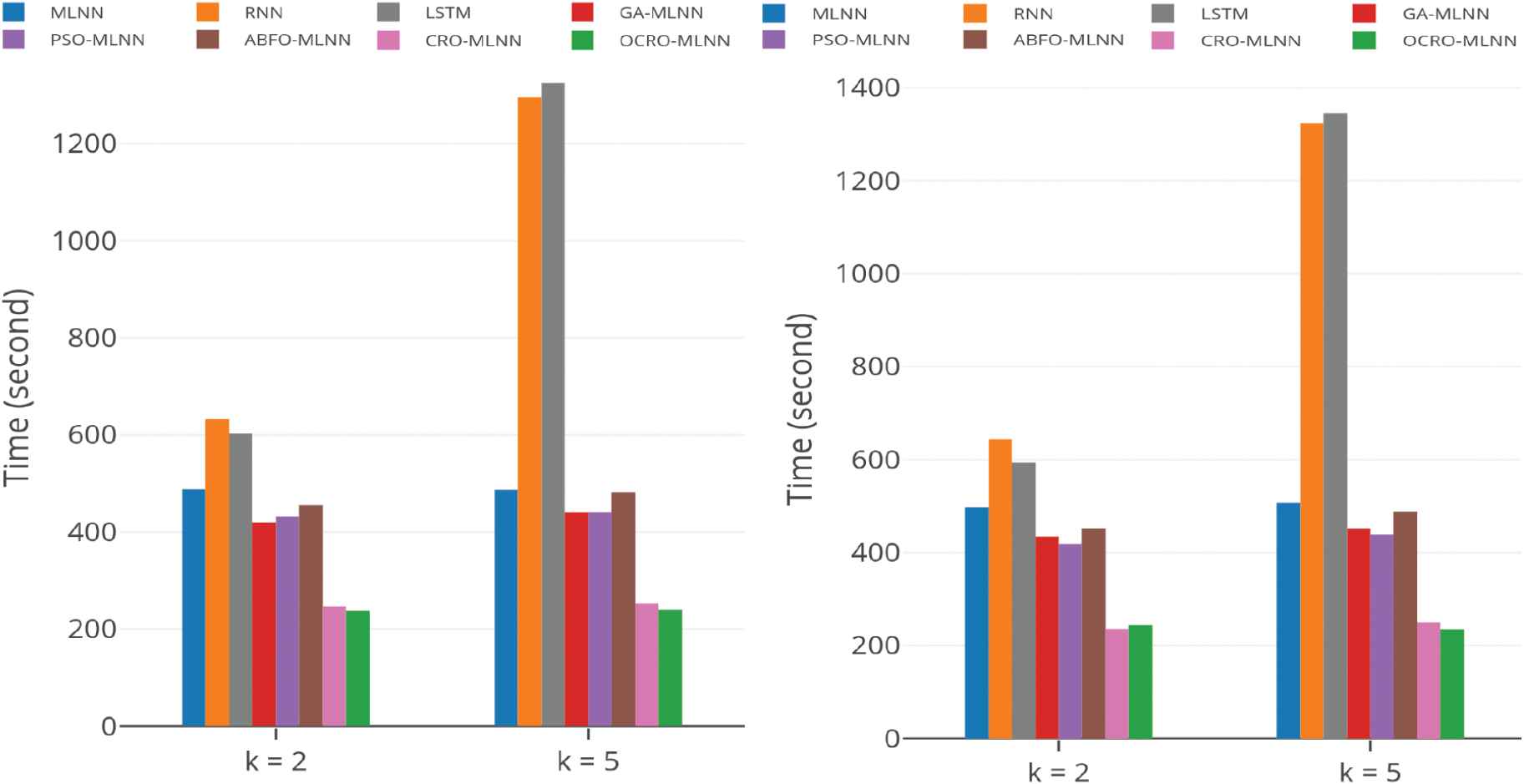
Runtime comparison: opposition-based coral reefs optimization (OCRO)-multi-layer neural network (MLNN) (green), sliding window = 5; univariate data: EU (left), WC (right).
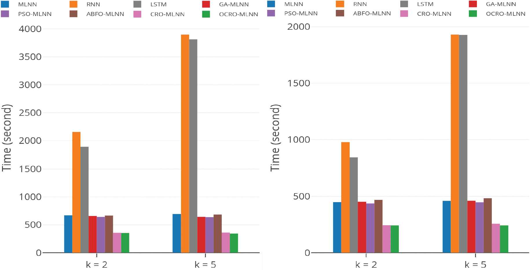
Runtime comparison. Table 6 presents outcomes of runtime experiments with different models. It can be seen that the obtained results of CRO-MLNN and OCRO-MLNN, which outperform other models on system runtime similarly as with univariate datasets. Concretely, for CPU metric with
| Data | Model | ||||||
|---|---|---|---|---|---|---|---|
| CPU | MLNN | 0.0973 | 0.5281 | 487.77 | 0.0971 | 0.5110 | 486.71 |
| GA-MLNN | 0.5999 | 0.0008 | 419.94 | 0.6300 | 0.0008 | 441.02 | |
| ABFO-MLNN | 0.6502 | 0.0007 | 455.11 | 0.6891 | 0.0011 | 482.37 | |
| PSO-MLNN | 0.6172 | 0.0010 | 432.03 | 0.6302 | 0.0011 | 441.13 | |
| CRO-MLNN | 0.3514 | 0.0008 | 245.96 | 0.3611 | 0.0041 | 252.78 | |
| RNN | 0.6306 | 2.3131 | 632.91 | 1.2935 | 2.4592 | 1295.96 | |
| LSTM | 0.6005 | 2.2273 | 602.73 | 1.3223 | 2.3590 | 1324.65 | |
| OCRO-MLNN | 0.3404 | 0.0009 | 238.28 | 0.3431 | 0.0009 | 240.21 | |
| RAM | MLNN | 0.0993 | 0.5809 | 498.00 | 0.1012 | 0.5904 | 507.65 |
| GA-MLNN | 0.6209 | 0.0007 | 434.62 | 0.6455 | 0.0008 | 451.85 | |
| ABFO-MLNN | 0.6462 | 0.0009 | 452.31 | 0.6976 | 0.0012 | 488.32 | |
| PSO-MLNN | 0.5976 | 0.0010 | 418.30 | 0.6262 | 0.0011 | 438.32 | |
| CRO-MLNN | 0.3359 | 0.0009 | 235.13 | 0.3574 | 0.0008 | 250.18 | |
| RNN | 0.6406 | 2.7545 | 643.35 | 1.3208 | 2.7987 | 1323.56 | |
| LSTM | 0.5912 | 2.4918 | 593.65 | 1.3428 | 2.7694 | 1345.54 | |
| OCRO-MLNN | 0.3483 | 0.0009 | 243.80 | 0.3351 | 0.0009 | 234.55 | |
Runtime comparison (sliding window
Runtime comparison: opposition-based coral reefs optimization (OCRO)-multi-layer neural network (MLNN) (green), sliding window = 5; multivariate data, CPU (left), RAM (right).

RMSE comparison: average of 15 times; univariate data: EU (left), world cup (WC) (right).
Model stability. Table 7 gives summary statistics of RMSE error with the tested models after 15 run times. The evaluations gained through these experiments with multivariate data include:
MLNN and RNN are quite unstable (as usually) due to back-propagation dependence on the initial weights. LSTM has smaller fluctuation of RMSE's error at the cost of its complex structure. Specifically, for CPU metrics,
The proposed approach is applying meta-heuristic OCRO to optimization problems gives more stability than gradient descent approach. The reason is that OCRO is considered as an efficient and powerful searching algorithm to help it jump out the local optimal and search for the best solution. So that when combining OCRO with traditional MLNN, the achieved model can work well under different conditions.
Compared to CPU metrics and
| Data | Model | k = 2 |
k = 2 |
||||||||
|---|---|---|---|---|---|---|---|---|---|---|---|
| CPU | MLNN | 0.4563 | 0.6579 | 0.5232 | 0.0615 | 0.1175 | 0.4659 | 0.7135 | 0.5896 | 0.0902 | 0.153 |
| RNN | 0.4461 | 0.5918 | 0.5059 | 0.0353 | 0.0698 | 0.4489 | 0.5503 | 0.465 | 0.0279 | 0.0599 | |
| LSTM | 0.4489 | 0.4929 | 0.4706 | 0.0171 | 0.0364 | 0.4499 | 0.4929 | 0.4732 | 0.0172 | 0.0364 | |
| GA-MLNN | 0.4392 | 0.4631 | 0.4523 | 0.0058 | 0.0129 | 0.4362 | 0.4863 | 0.4557 | 0.0148 | 0.0324 | |
| PSO-MLNN | 0.4421 | 0.4605 | 0.4494 | 0.0055 | 0.0121 | 0.4444 | 0.4627 | 0.4537 | 0.0064 | 0.0142 | |
| ABFO-MLNN | 0.4423 | 0.5788 | 0.5119 | 0.0424 | 0.0829 | 0.4505 | 0.6528 | 0.5302 | 0.0596 | 0.1124 | |
| CRO-MLNN | 0.4386 | 0.4545 | 0.4485 | 0.004 | 0.009 | 0.4428 | 0.4634 | 0.4503 | 0.0051 | 0.0114 | |
| OCRO-MLNN | 0.4392 | 0.4523 | 0.4474 | 0.0028 | 0.0064 | 0.4396 | 0.4571 | 0.4492 | 0.0058 | 0.0128 | |
| RAM | MLNN | 0.0334 | 0.0676 | 0.0436 | 0.0103 | 0.2363 | 0.0326 | 0.0676 | 0.0528 | 0.0091 | 0.173 |
| RMM | 0.0323 | 0.0446 | 0.0372 | 0.0037 | 0.1008 | 0.0323 | 0.0414 | 0.0363 | 0.0031 | 0.0868 | |
| LSTM | 0.0318 | 0.0346 | 0.0327 | 0.001 | 0.0293 | 0.0318 | 0.0398 | 0.0331 | 0.0019 | 0.0583 | |
| GA-MLNN | 0.031 | 0.0331 | 0.0321 | 0.0005 | 0.0156 | 0.032 | 0.0363 | 0.0336 | 0.0013 | 0.0389 | |
| PSO-MLNN | 0.0309 | 0.0342 | 0.0322 | 0.0008 | 0.0259 | 0.0314 | 0.0348 | 0.0325 | 0.0009 | 0.0291 | |
| ABFO-MLNN | 0.0322 | 0.0541 | 0.0414 | 0.0064 | 0.1549 | 0.0313 | 0.0537 | 0.0395 | 0.0082 | 0.2065 | |
| CRO-MLNN | 0.0313 | 0.033 | 0.0322 | 0.0005 | 0.0154 | 0.0312 | 0.0335 | 0.0324 | 0.0007 | 0.0222 | |
| OCRO-MLNN | 0.031 | 0.0328 | 0.0322 | 0.0005 | 0.0149 | 0.0312 | 0.0336 | 0.0324 | 0.0007 | 0.0218 | |
RMSE comparison (average of 15 times; multivariate dataset).
Figure 10 expresses average RMSE after 15 run times of all models (the same way as univariate dataset).
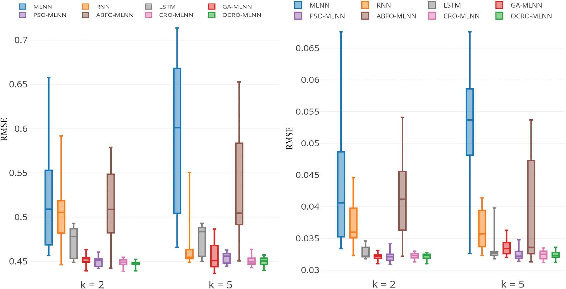
Root mean square error (RMSE) comparison: average of 15 times; multivariate data: central processing unit (CPU) (left), RAM (right).
5.3. Practical Usage of the Proposed Forecasting Approach
In the distributed environment, one of the core issues is how to optimize scheduling resources under heavy and changeable computation loads that are made by complex requirements coming from applications. With a set of available resources (e.g. servers, networks, storages), a scheduler (74) must have the capability to make scale in/out decisions to provide computation powers for those applications. Although the traditional technique for the scaling problem with predefined resource usage thresholds is employed widely in fact, this method has the main disadvantage in operation and management of distributed applications: there is always latency between the decision-making moment and its efficiency. This leads to the resources offered to applications does not match with demand in real-time. To deal with the issue, scheduler deployed in distributed systems requires precise estimates resource consumptions. To achieve that capability, the scheduler must have a certain component to predict expected performances of infrastructure systems. The forecast module also is designed in the manner of minimizing costs such as simple prediction model, stability, and runtime constraint, but keeping the good accuracy in order to well operate in practice.
Within our work in this direction, the prediction-based auto-scaling systems for cloud resource management was considered in [44] taking into account quality of service (QoS) defined in service-layer agreements (SLA). The aim is to reduce cloud resource over-provisioning that causes wasted energy consumption as well as e-infrastructure production cost. The cloud resources provision under SLA conditions is extended in [49] with experimental results to ensure QoS using the number of provided virtual machines (VMs) instead of cloud monitoring metrics to make scaling decisions. The work presented in this paper continues in improvements of the intelligent module functionalities. It is oriented not only for resource management but also for network traffic monitoring.
With the application direction presented above, in this work, through experiments, we proved our proposed OCRO-MLNN model can be applied to schedulers in distributed systems to resolve the scaling issue. Moreover, the model also brings efficiency as desired as compared with other modern learning techniques. Indeed, the tested data was collected from the computing infrastructures (i.e. Google's cluster workload and Internet traffic) and distributed applications (Football world cup's website connection) is used to carry out the model evaluation experiments.
6. CONCLUSION AND FUTURE WORKS
This work presented an approach and technique for prediction problem with time series data. The approach is based on the idea to build a stable model with simple structure, low run-time training, but still brings good accuracy as compared with other modern models. In this way, we created a novel algorithm called opposition-based coral reefs optimization (OCRO). Specifically, the proposed algorithm is the combination of CRO using OBL. Thus, we used OCRO together with the MLNN to deal with the forecast problem in the nonlinear time series data. By the improvement, our OCRO-MLNN reducing complexity of the model due to faster convergence in comparison with the back-propagation technique.
We are interested in applying the created OCRO-MLNN to distributed systems in order to increase the effectiveness as well as efficiency in allocating resources for applications in the manner of proactiveness. Due to its simplification, fast training, stabilization, and forecast performance, the proposed model has the feasibility in applying to the resource schedulers. With the application direction of using in distributed systems, we already tested the proposed OCRO-MLNN with real dataset gathered from those systems, including Google trace cluster data, Internet traffic, and popular website's connections. The achieved results through experiments shown that our OCRO-MLNN has advantages in all the proposed criteria listed above as compared with other state-of-the-art models in both univariate and multivariate data. This proves OCRO-MLNN's feasibility in applying to real systems (e.g. clouds, decentralized ledgers applications etc.) in practice.
The study made contributions in four areas. First, we built the OCRO technique by using OBL mechanism for CRO. The improvement helps searching process and avoid the local minimum of traditional CRO. Second, a novel forecast model is introduced with the combination of our OCRO technique with MLNN. In which OCRO is used to replace back-propagation. Third, in terms of evaluation, we conducted comparisons among different prediction models and OCRO-MLNN for time series data. Four, with three real datasets collected from well-known systems, we tested the performance of the proposed model as well as other popular methods above. The tests were carried out under three factors, including accuracy, stability, and runtime.
In the future, there are two routes that we plan to do. The first route is to design and develop a resource allocation scheduler which we would like to employ to decentralized systems. In our project funded by VINIF, we have deployed an auto-scaler for controlling computation resources for blockchain nodes of the V-Chain platform using ORCO-MLNN prediction model proposed in this work. The goal of this use is to optimize cloud resource consumption as well as monitor network bandwith of the system. The scheduler thus must process multivariate data with diverse metrics as usual scaling requirement. Besides, a resource allocation decision module also is demanded for the scheduler. The second route is to use and improve several other nature-inspired algorithms, then combine with machine techniques like neural network to serve forecast problem in proactive auto-scalers of distributed systems.
CONFLICT OF INTEREST
The authors declare no conflict of interest.
AUTHORS' CONTRIBUTIONS
T. Nguyen and Tu Nguyen designed the program; T. Nguyen, Tu Nguyen, and B.M. Nguyen tested; T. Nguyen, Tu Nguyen, and B.M. Nguyen prepared and wrote the original draft; B.M. Nguyen and G. Nguyen reviewed and edited; and B.M. Nguyen conducted the project administration.
ACKNOWLEDGMENT
Research is supported by Vingroup Innovation Foundation (VINIF) in project code VINIF.2019.DA07.
REFERENCES
Cite this article
TY  - JOUR
AU  - Thieu Nguyen
AU  - Tu Nguyen
AU  - Binh Minh Nguyen
AU  - Giang Nguyen
PY  - 2019
DA  - 2019/11/04
TI  - Efficient Time-Series Forecasting Using Neural Network and Opposition-Based Coral Reefs Optimization
JO  - International Journal of Computational Intelligence Systems
SP  - 1144
EP  - 1161
VL  - 12
IS  - 2
SN  - 1875-6883
UR  - https://doi.org/10.2991/ijcis.d.190930.003
DO  - 10.2991/ijcis.d.190930.003
ID  - Nguyen2019
ER  -