
A Hybrid Global Optimization Algorithm Based on Particle Swarm Optimization and Gaussian Process
- DOI
- 10.2991/ijcis.d.191101.004How to use a DOI?
- Keywords
- Swarm optimization; Gaussian process; Global optimization; Surrogate approach
- Abstract
The optimization problems and algorithms are the basics subfield in artificial intelligence, which is booming in the almost any industrial field. However, the computational cost is always the issue which hinders its applicability. This paper proposes a novel hybrid optimization algorithm for solving expensive optimizing problems, which is based on particle swarm optimization (PSO) combined with Gaussian process (GP). In this algorithm, the GP is used as an inexpensive fitness function surrogate and a powerful tool to predict the global optimum solution for accelerating the local search of PSO. In order to improve the predictive capacity of GP, the training datasets are dynamically updated through sorting and replacing the worst fitness function solution with the better solution during the iterative process. A numerical study is carried out using twelve different benchmark functions with 10, 20 and 30 dimensions, respectively. Regarding solving of the ill-conditioned computationally expensive optimization problems, results show that the proposed algorithm is much more efficient and suitable than the standard PSO alone.
- Copyright
- © 2019 The Authors. Published by Atlantis Press SARL.
- Open Access
- This is an open access article distributed under the CC BY-NC 4.0 license (http://creativecommons.org/licenses/by-nc/4.0/).
1. INTRODUCTION
Swarm intelligence [1–4] was identified as a promising new optimization technique over the past decade. It is an attempt to develop algorithms inspired by the collective behavior of social insects and other animal societies. There are many swarm intelligence approaches designed for algorithmic optimization, such as cuckoo search algorithm [5–6], bat algorithm [7–8], artificial bee colony algorithm [9], fish school algorithm [10], ant colony optimization algorithms [11] and particle swarm optimization (PSO) algorithms [12–14]. Though most of swarm intelligence share the similar concept on collective behavior of decentralized, self-organized systems, natural or artificial, each swarm intelligence-based algorithm has its characteristic. Therefore, the different swarm intelligence algorithm could be assigned in different application to maximize the performance. For example, Cuckoo search idealized such breeding behavior, and thus can be applied for series system in hardware design [15]. Bat algorithm mimics a frequency-tuning method to control the dynamic behavior thus can be used to design the transport network [16]. Herein, the PSO as a more general approach developed by Eberhart and Kennedy in 1995 has better applicability over the others. The PSO is a metaheuristic as it requires few or no assumptions about the problems; therefore, it can search very large space of candidate solutions [17]. In the search space, the position and velocity of particle motion will be equated by simple mathematical expression. Specifically, the form of path is relinked among optimal position (pbest). In this sense, PSO shares many similarities with evolutionary computation techniques such as genetic algorithms (GAs) [18]. Compared to GA, PSO has fewer parameters to adjust and better convergence capability for the complex optimization problems [19]. However, like other population-based algorithms, PSO has some inevitable disadvantages, for example, it is difficult in defining initial parameters; this method is not applicable for the problems of scattering and it can be trapped into a local minimum especially with complex problems. More important, PSO requires a large number of fitness function evaluations. Moreover, aiming to practical engineering problems, the real function is usually missing. Therefore, the numerical simulation is introduced to build the explicit relationship between variable and fitness [20,21]. But it is often infeasible to apply the process to fitness evaluation due to its high computational cost. Examples of such problems include large-scale finite element method analysis or computational fluid dynamics simulations [22]. In such problems, a single exact fitness function evaluation (involving the analysis of a complex engineering system based on high fidelity simulation codes) often consumes massive CPU time. Therefore, the high computational cost involved posing a serious impediment to PSO's successful application.
In order to reduce the computational cost of PSO, many methods have been considered and implemented. GA can be used to modify the decision vector to speed up the procedure [23,24]. By applying the binary variables, the PSO can be adapted to consume less computational cost [25]. However, more promising way to significantly reduce the computational cost of PSO is to employ computationally cheap surrogate model or metamodel in place of computationally expensive exact fitness evaluations. The metamodel as a surrogate model is constructed by generating a set of data points in the design space and evaluating the cost function. This method relies on establishing the accurate metamodel. For example, Praveen and Duvigneau [26] developed a low cost PSO by using metamodels to simulate the aerodynamic shape. Selleri et al. [27] try to optimize the array in the design of antennas and microwave by introducing metamodel to PSO. Besides metamodels, research on surrogate-assisted evolutionary computation began over a decade ago and had received considerably more interest in recent years [28–32]. In the surrogate approach, a surrogate model is trained on existing evaluated individuals (fitness cases) in order to guide the search for promising solutions. Biswas et al. [33] coupled the Bacterial Foraging Optimization Algorithm (BFOA) with PSO for optimizing multimodal and high-dimensional functions. Zhang et al. [34] employed the artificial immune system (AIS) and chaos operator as a surrogate to lower the computational cost in PSO. By leveraging surrogate models, the number of expensive fitness evaluations decreases, which result in significant decrease in computational cost [35–37]. Though currently a variety of empirical models can be used to construct the approximation (e.g., polynomial models (PMs), artificial neural networks (ANNs) and radial basis function networks (RBFNs)), there are still limitations which are difficult to be overcome (i) for the surrogate models, PM can't cope with large dimensional multimodal problems since they generally carry out approximation using simple quadratic models; ANN always has difficulty in finding an appropriate network topology and the optimum hyperparameter; a major difficulty in RBFN is to set the optimum decay parameter. Therefore, there is an urgent need to develop a novel framework to solve those problems. (ii) In respect to the strategies of algorithms, the performance of the algorithms is highly dependent on the quality of training data. Generally speaking, to achieve a valid surrogate model, the data for training must be “representative” of the overall design space and the global optimum solution should be included in the interval of training data. Nevertheless, the training dataset for training surrogate models remain unchanged during the whole searching process. To this end, the conventional strategy does not guarantee that the selected training dataset covers the entire design space or the global optimum solution locates in the interval of training data, especially for the scenarios with large variables but with limited training datasets. So, the surrogate models are very easy to be trapped by the local optimum solution if the training datasets are not selected properly.
Gaussian process (GP) can directly capture the model uncertainty; and also, it is be able to add prior knowledge and specifications about the shape of the model by selecting different kernel functions. Therefore, it is suitable to introduce the Gaussian mutation to PSO to improve the efficiency. Higashi and Iba [38] demonstrate a way to combine PSO with GP. The proposed strategy achieves better performance than PSO itself. Krohling [39] developed a Gaussian PSO algorithm to solve the multimodal optimization problems. But the PSO still can be stuck in local minima when optimizing functions. The key to adapt GP in PSO is to find the proper optimal combination strategy. In this process, for most of current methods, it excessively relies on the sample if the approximate model is directly replaced with the fitness function. In particular, the accuracy of regression is determined by the sample. If the representation of learning sample is either poor or off from the global trend, the corresponding accuracy of prediction will be low, leading failed in search optimal value.
In order to overcome the problems described above, a novel hybrid GP surrogate-assisted PSO optimization algorithm is proposed in this paper. Comparing with the conventional surrogate models, the proposed algorithm has merits in the following aspects: (i) training datasets are generated randomly; (ii) the local search is accelerated; (iii) the training datasets can be dynamically updated. To sum up, the proposed algorithm can guarantee the accuracy and efficiency for solving computationally expensive global optimization problems. For convenience, the proposed algorithm will be named as GP-PSO. The remainder of this paper is structured as follows: Section 2 gives a brief introduction of the related methodology including PSO and GP; Section 3 presents the proposed GP-PSO algorithm; Section 4 demonstrates the validity and efficiency of the proposed algorithm by experiments. Finally, the conclusions and future works are presented in Section 5.
2. REVIEW OF RELATED METHODOLOGY
2.1. Particle Swam Optimization
PSO is initialized with a population of random solutions and searches for optima by updating generations. In PSO, the potential solutions, called particles, fly through the problem space by following the current “optimum” particles. There are two “optimum” particles: one keeps track of its coordinates associated with the best solution in current stage. The best solution is defined as pbest. The other “best” tracked by the particle swarm optimizer is obtained so far by any particle in the neighbors of the particle. When a particle takes all the population as its topological neighbors, this global best denoted as gbest. With the help of the two best values, the particle updates its velocity and positions with following equation:
2.2. Gaussian Process
For the approximation of the fitness function we chose GP, which is a newly developed machine learning technology based on strict theoretical fundamentals and Bayesian theory [43]. In recent years, GP has attracted much attention in the machine learning community [44–46]. Like ANNs, which are the most prominent surrogate models, GP can approximate any function. During searching the optimum solution by PSO, a GP model is used to approximate the real function, so that the number of evaluations of real functions can be dramatically reduced. Compared to ANN, GP's main advantage is the simplicity: no need to choose network size or topology. Besides, GP can automatically choose the optimum hyper-parameters. More details about GP can be seen in the work by Rasmussen and Williams [47].
A GP is a collection of random variables, any finite set of which have a joint Gaussian distribution. A GP is completely specified by its mean function m(x) and the covariance function
There is a training set D of m observations,
GP procedure can handle interesting models by simply using a covariance function with an exponential term:
The log-likelihood and its derivative with respect to
Hyper-parameters
3. THE PROPOSED GP-PSO ALGORITHM
In this paper, in order to improve the PSO's efficiency for computationally expensive optimization problem, a GP-based PSO algorithm is developed. In GP-PSO algorithm, GP is applied to approximate the real function. Once the approximation function is found, we can directly use the approximation function instead of real function to evaluate the fitness of the particles. Hence, the number of real function evaluations can be reduced greatly by using PSO to solve the optimization problem. Key points of GP-PSO algorithm are the following:
Accelerate searching based on approximating real function by GP
In order to accelerate the local search of PSO, once the pbest particle and gbest particle in each iterative step are found, some new particles are generated using Eq. (1) and their fitness are estimated by trained GP. Then the best one with the minimum fitness is selected. To eliminate the predictive error of fitness evaluated by GP approximation, the fitness of the best particle is evaluated again using the real function. If the real fitness of the best one is less than gbest, it becomes the global best in current iterative step and gbest is replaced by its fitness. Thus, the number of real function evaluations in exploration process is only one because the fitness of the new particles with the exception of the best one is evaluated by trained GP rather than real function. So the computational cost of the process of accelerating search is low.
Dynamically update the training datasets to improve approximation quality of GP model
The accuracy of GP-PSO algorithm depends on the appropriateness of the GP model generated, while in aspect of prediction, the accuracy of the GP model in interpolation and validity highly depend on the quality of training datasets. To avoid excessively relying on the initial training datasets and to improve the quality of training datasets gradually in the exploration process, the training datasets for training GP is updated dynamically in GP-PSO algorithm. The strategies can be realized through the following two ways:
In each iterative step of PSO, particles of all generation are ranked from small fitness to large fitness, the top 2×N particles and their real fitness are selected as training datasets by multiple try-and-error, where N is the population size. In this case, the Rastrigin function was selected as benchmark due to its high complexity. Through comparison of different dimension of particles (from N to 3×N), 2×N was used because it resulted in lowest computational cost on condition of the required accuracy.
In each iterative step of PSO, the best particle and its fitness is found by local search, which is based on evaluation of the function generated by the GP model, the worst particle in training datasets is replaced with the best one.
Thus the training datasets are always consistent with the elite group of the particles, the quality of general approximation of GP model can be enhanced in the optimization process. Specifically speaking, the implementation procedure is presented in this section associated with the flow chart, see in Figure 1. Its framework mainly consists of two cycles. The cycle depending on “p” is defined as outer loop and the cycle depending on “k” is defined as inner loop. Meanwhile, the initial values for both p and k are zero.
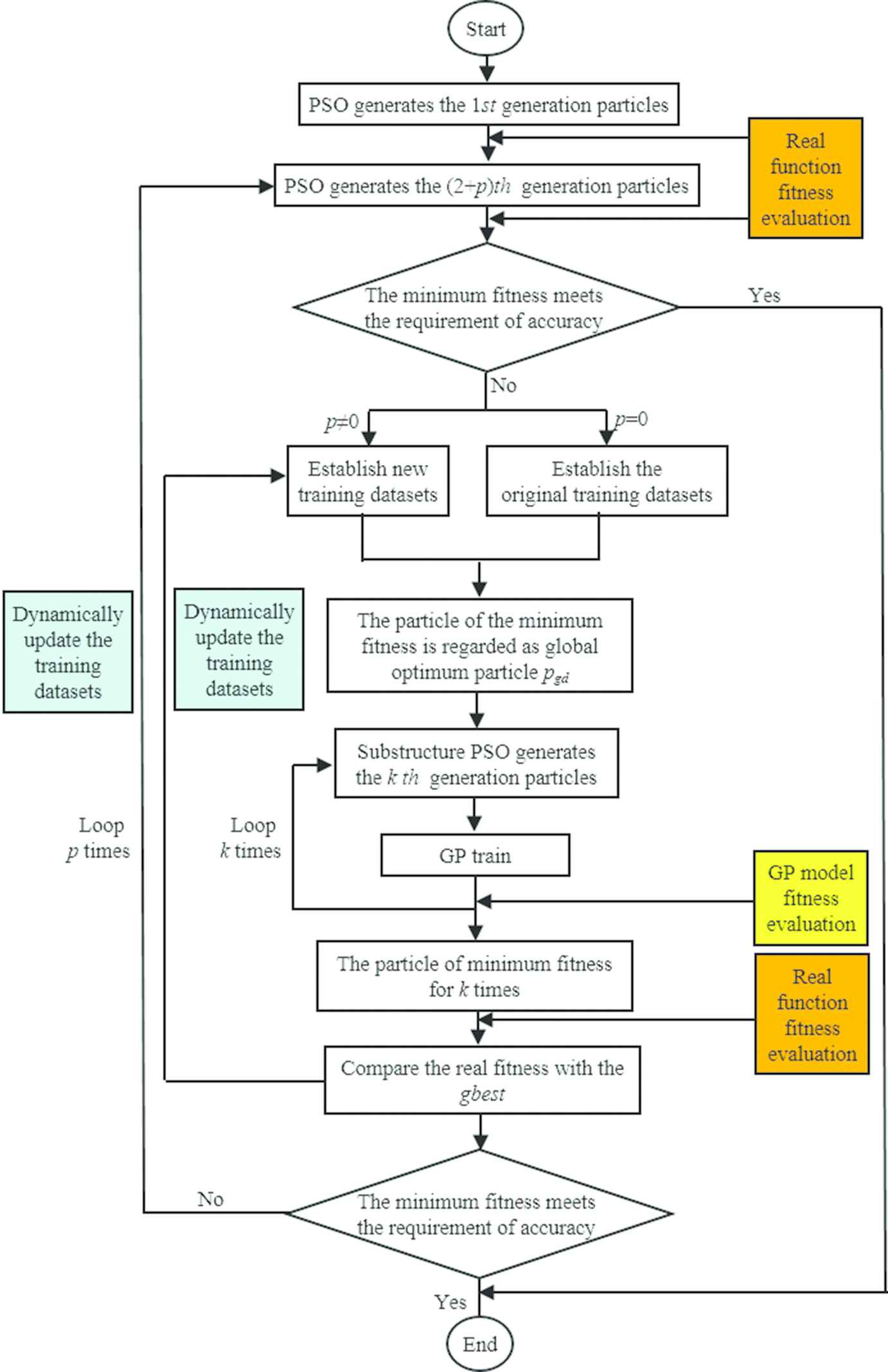
The flow chart of Gaussian process-particle swarm optimization (GP-PSO).
Specific implementation steps of GP-PSO are shown as follows:
Generate N particles in the 1st generation, in which the particles are randomly distributed throughout the design space, which is bounded by specified limits. N is the population size of PSO, it is usually determined by the dimension of optimization problem.
Evaluate the fitness of particles of 1st generation by objective function, i.e., real function. Find the optimum particle pid and global optimum particle pgd.
Generate N particles of (2+p)th generation using Eq. (1). Evaluate the fitness of these particles using real function.
The (2+p)×N particles are sorted from small fitness to large fitness, and the upper limit 2×N particles and their fitness are selected to establish training datasets.
Train GP by the training datasets. Use GP approximate the real function according to Eq. (5).
Update the optimum particle pid and global optimum particle pgd at current iteration.
Generate k×N particles using Eq. (1) and evaluate the fitness of N particles using trained GP. Find the best particle with the minimum fitness in k generation, where k can make the best particle more optimizing, k is determined by the complexity of the real function. The more complex the real function is, the greater the value of k will be. Evaluate its fitness using real function and replace its fitness evaluated using trained GP. Compare its fitness to gbest, select the smaller one as global optimum particle pgd and update gbest.
Replace the worst particle with the maximum fitness in training datasets by the global optimum particle and its fitness gbest.
Repeat steps 3–8 until the stopping criteria is met. For the current implementation the stopping criteria is defined based on the maximum number of iterations reached or accuracy satisfied.
The pseudo code of GP-PSO is given in Figure 2. A MATLAB based program was developed.
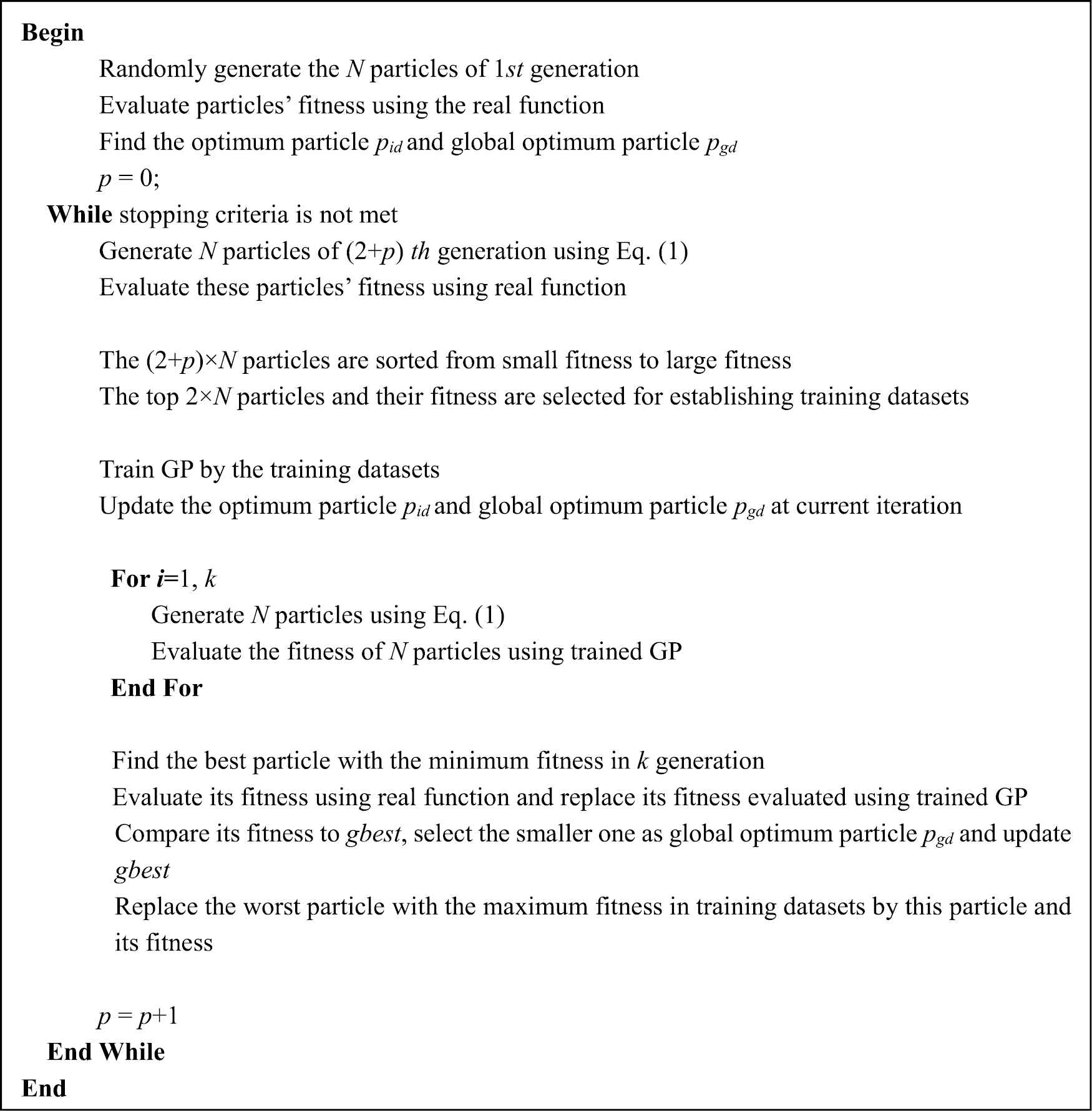
Pseudo code of Gaussian process-particle swarm optimization (GP-PSO).
4. EXPERIMENTS
4.1. Benchmark Functions
The performance of the GP-PSO algorithm was compared to the conventional PSO algorithm by evaluating convergence velocity and efficiency for benchmark optimization problems. 12 popular benchmark functions are selected in Table 1. It includes 8 unimodal benchmark functions and 4 multimodal benchmark functions. For all functions in Table 1, the minimal function value is f = 0 and search space is confined to [−2, 2]d, here d denotes the dimension of the functions.
| Function | Formulation | Trait | Search Range |
|---|---|---|---|
| Sphere | Unimodal | [−2,2]d | |
| Ellipsoid | Unimodal | [−2,2]d | |
| Step | Unimodal | [−2,2]d | |
| Sumsquares | Unimodal | [−2,2]d | |
| Cigar | Unimodal | [−2,2]d | |
| Tablet | Unimodal | [−2,2]d | |
| Rosen | Unimodal | [−2,2]d | |
| Quartic | Unimodal | [−2,2]d | |
| Ackley | Multimodal | [−2,2]d | |
| Schwefel | Multimodal | [−2,2]d | |
| Griewank | Multimodal | [−2,2]d | |
| Rastrigin | Multimodal | [−2,2]d |
Parameter settings of the benchmark functions.
The Sphere, Ellipsoid, Step and Sumsquares functions are unimodal, convex and differentiable without flat regions. The Cigar, Tablet and Rosen functions have a single global minimum located in a long narrow parabolic shaped flat valley, what's more, it is very hard to find global optimum. Quartic function is unimodal with random noise. Noisy functions are widespread in real-world problems, and every evaluation for the function is disturbed by noise, so the particles' information is inherited and diffused noisily, which makes the problem hard for optimization [49].
Multimodal functions evoke hills and valleys, which are misleading local optima. Schwefel and Ackley have large amount of local minima causing difficulties in finding the global optimum. The Griewangk and Rastrigin are highly multimodal test functions, which are usually used to evaluate the efficiency of optimization algorithm.
For the benchmark functions, we measure the number of the real function evaluation which is required to achieve expected accuracy.
4.2. Parameter Setting
The parameters for PSO include population size (N), lower (lb) and upper (ub) bounds of the search space, maximum number of iterations (tmax), inertia parameter (w), maximum velocity of particle (vmax) and acceleration constants (c1 and c2). For different dimension problem, some parameters remain unchanged: lb = −2, ub = 2, vmax = 1, c1 = c2 = 2. The values of N and tmax are listed in Table 2. The maximum number of circular for accelerating local search k = 10.
| Function | 10 Dimensions |
20 Dimensions |
30 Dimensions |
||||||
|---|---|---|---|---|---|---|---|---|---|
| N | tmax | Accuracy | N | tmax | Accuracy | N | tmax | Accuracy | |
| Sphere | 30 | 2000 | 1.00E-03 | 30 | 8000 | 1.00E-03 | 50 | 20000 | 1.00E-03 |
| Ellipsoid | 30 | 2000 | 1.00E-03 | 30 | 8000 | 1.00E-03 | 50 | 20000 | 1.00E-03 |
| Step | 30 | 2000 | 1.00E-03 | 30 | 8000 | 1.00E-03 | 50 | 20000 | 1.00E-03 |
| Sumsquares | 30 | 2000 | 1.00E-03 | 30 | 8000 | 1.00E-03 | 50 | 20000 | 1.00E-03 |
| Cigar | 30 | 2000 | 1.00E-03 | 30 | 8000 | 1.00E-03 | 50 | 20000 | 1.00E-03 |
| Tablet | 30 | 2000 | 1.00E-03 | 30 | 8000 | 1.00E-03 | 50 | 20000 | 1.00E-03 |
| Rosen | 30 | 10000 | 3.00E+01 | 30 | 20000 | 3.00E+01 | 50 | 50000 | 3.00E+01 |
| Quartic | 30 | 10000 | 1.00E-01 | 30 | 20000 | 1.00E-01 | 50 | 50000 | 1.00E-01 |
| Ackley | 30 | 2000 | 1.00E-03 | 30 | 8000 | 1.00E-03 | 50 | 20000 | 1.00E-03 |
| Schwefel | 30 | 2000 | 1.00E-03 | 30 | 8000 | 1.00E-03 | 50 | 20000 | 1.00E-03 |
| Griewank | 30 | 2000 | 1.00E-03 | 30 | 8000 | 1.00E-03 | 50 | 20000 | 1.00E-03 |
| Rastrigin | 30 | 10000 | 3.00E+01 | 30 | 20000 | 3.00E+01 | 50 | 50000 | 3.00E+01 |
GP, Gaussian process; PSO, particle swarm optimization.
Parameter settings of GP-PSO and PSO.
To be fair, for different functions, all algorithms are forced to use the same accuracy of stopping criteria; for different functions, there is different accuracy for stopping criteria which is listed in Table 2. The program for all experiments runs over 30 times independently then the number of function evaluation are averaged finally.
In order to validate the scalability of our algorithm, all functions are tested on 10, 20 and 30 dimensions, respectively [50].
4.3. Parameter Selection
In the optimization, the selection of parameters can significantly influence on the performance of the proposed algorithm. In this section, some essential parameters are discussed, and how they impact on the optimization results are forecasted. Afterward, the recommendations are provided accordingly.
lb and ub are the lower and upper bounds of the search space, respectively. They are distributed symmetrically about the searching value. In this paper the minimal function value is 0, so the search space is confined to [−2, 2]. The computational cost will increase with the interval between lb and ub; specifically speaking, if it is too small (i.e., [−0.1, 0.1]), any optimization method can easily find the optimal results, that can't be used for evaluating the performance differences between different methods. In this paper, the aim for this benchmark optimization problem is to compare the performance of the GP-PSO algorithm and PSO algorithm. As long as the performance of the two algorithms can be compared under the same condition, the smaller interval is used to save the computational time. Therefore, the bound of [−2, 2] is big enough to compare the performance of the GP-PSO algorithm and PSO algorithm.
vmax is a parameter specified by the user, then the velocity on that dimension is limited to vmax. vmax determines the resolution of the search regions between the present and target position. The PSO works well if vmax is set to the value of the dynamic range of each variable (on each dimension). The dynamic range is [−2, 2] in this paper, so we choose the vmax = 1.
c1 and c2 are acceleration constants usually defined as c1 = c2 = [1.8, 2.0], that can be found in literature [41]. Any value in this interval could be chosen. In this paper, we choose c1 = c2 = 2.0.
N is usually determined by the difficulty of the optimization problem. Small population size results in unreliable results, while the large size will increase computational cost and may cause slow convergence. The population size should be selected with the consideration of the tradeoff between the solution quality and the computation time. It is always determined by the experience. In this paper, we choose the N based on the following reference [51]. In this reference, 10, 30, 50, 80 and 100 population sizes are used to solve the optimization problem, respectively. In our work, the purpose is to evaluate the performance of two algorithms. Therefore, in order to find a balance between accuracy and computational cost, the value is selected as 30 and 50 depending on the complexity of the optimization problem.
tmax determines the maximum run times of algorithm. Because all the different algorithms are forced to use the same accuracy as the termination criterion, the tmax should be big enough to make the algorithms meet the termination criterion. There is no certain limit of this parameter. For example, the Sphere function is relatively simple, so 2000 is sufficient; meanwhile, the Rastrigin function is more complex, 50000 is adapted.
k represents the increment of loop as substructure of PSO algorithm. In GP-PSO, the GP is used as an inexpensive fitness function surrogate and a powerful tool to predict the global optimum solution for accelerating the local search of PSO. The fitness of total k generations doesn't need to be calculated; instead, it is predicted by GP model. Usually, the prediction of GP approximates to the optimal solution by using larger k. However, larger k also causes high computational cost. Therefore, k = 10 in our paper is determined, which can satisfy our optimal requirement. In conclusion, all of the parameters mentioned are summarized in Table 3.
| Parameter | Influence | Recommendation |
|---|---|---|
| lb | Computational cost | −2 |
| ub | Computational cost | 2 |
| vmax | Convergence | 1 |
| c1 | Accuracy, computational cost and convergence | 2 |
| c2 | Accuracy, computational cost and convergence | 2 |
| N | Accuracy, computational cost and convergence | 30 or 50 |
| tmax | Convergence | 2000–50000 |
| k | Computational cost and convergence | 10 |
The summation of parameter selection.
4.4. Results Analysis
The total number of the real function evaluation using GP-PSO and PSO are shown in Table 4, respectively. It can be seen from Table 4, total number of real function evaluation in GP-PSO is much less than that PSO requires.
| Function | 10 Dimensions |
20 Dimensions |
30 Dimensions |
||||||
|---|---|---|---|---|---|---|---|---|---|
| PSO | GP-PSO | Multiple | PSO | GP-PSO | Multiple | PSO | GP-PSO | Multiple | |
| Sphere | 22230 | 1549 | 14 | 92550 | 9299 | 10 | 427400 | 32129 | 13 |
| Ellipsoid | 25140 | 2572 | 10 | 106440 | 12306 | 9 | 435100 | 48704 | 9 |
| Step | 24360 | 2014 | 12 | 94800 | 7439 | 13 | 388900 | 33659 | 12 |
| Sumsquares | 24180 | 2200 | 11 | 95280 | 8524 | 11 | 440750 | 52733 | 8 |
| Cigar | 29610 | 4680 | 6 | 118650 | 16398 | 7 | 476850 | 65075 | 7 |
| Tablet | 24180 | 2076 | 12 | 98130 | 8276 | 12 | 426250 | 41462 | 10 |
| Rosen | 1260 | 154 | 8 | 110880 | 2975 | 37 | 816150 | 41819 | 20 |
| Quartic | 20070 | 743 | 27 | 139050 | 4370 | 32 | 847100 | 28610 | 30 |
| Ackley | 29580 | 4215 | 7 | 112470 | 14817 | 8 | 470900 | 56609 | 8 |
| Schwefel | 23520 | 4184 | 6 | 101610 | 17886 | 6 | 471850 | 62474 | 8 |
| Griewank | 16950 | 774 | 22 | 73620 | 4711 | 16 | 343900 | 19175 | 18 |
| Rastrigin | 810 | 278 | 3 | 114780 | 867 | 132 | 802050 | 10862 | 74 |
GP, Gaussian process; PSO, particle swarm optimization.
Comparison of the number of function evaluation between GP-PSO and PSO.
For 10-, 20-, 30-dimensional benchmark functions, the average multiple of the real function evaluation is about 12, 24, 18 times, respectively, the minimum multiple of it is 3 times (Rastrigin function with 10 dimension), and the maximum multiple of the real function evaluation is 132 times (Rastrigin function with 20 dimension).
In order to evaluate the performance of the proposed algorithm, the Rastrigin and Rosen function with 30 dimensions was used due to their high difficulty in searching optimal value. Usually, the mean value and corresponding standard deviation are two important features to evaluate the accuracy and robustness of algorithm. The GP-PSO was compared with PSO, PSO-w-local [52] and PSO-cf-local [53], respectively. The results are summarized in the Table 5. Except for PSO-cf-local, the mean value calculated from the other three algorithms approach to the actual value of 30 for both Rastrigin and Rosen function. The PSO-cf-local has the lowest accuracy in our case. The proposed GP-PSO can achieve the same accuracy of PSO and PSO-w-local. However, it has the lowest standard deviation. That means the proposed GP-PSO algorithm has better performance in robustness in the premise of sufficient accuracy.
| Algorithm | Rastrigin |
Rosen |
||||||
|---|---|---|---|---|---|---|---|---|
| Best | Worst | Mean | Std | Best | Worst | Mean | Std | |
| PSO | 2.97E+01 | 3.00E+01 | 2.99E+01 | 1.90E-01 | 2.93E+01 | 3.00E+01 | 2.96E+01 | 3.10E-01 |
| PSO-w-local [52] | 2.09E+01 | 3.38E+01 | 2.64E+01 | 4.08E+00 | 2.41E+01 | 2.94E+01 | 2.60E+01 | 2.26E+00 |
| PSO-cf-local [53] | 2.89E+01 | 6.17E+01 | 4.03E+01 | 1.20E+01 | 1.77E+01 | 2.32E+01 | 1.95E+01 | 2.44E+00 |
| GP-PSO | 2.94E+00 | 3.00E+01 | 2.97E+01 | 8.00E-02 | 2.91E+01 | 3.00E+01 | 2.95E+01 | 2.80E-01 |
GP, Gaussian process; PSO, particle swarm optimization.
Comparison results of GP-PSO with other algorithms for 30-dimensional problems.
In order to give a visualized and straightforward comparison between the proposed GP-PSO and PSO, the comparison of the performances of GP-PSO and PSO for 30-dimensional benchmark functions are shown in Figure 3. In the figures, the convergence trends of variants of PSO and GP-PSO in a random run can be identified. These figures show that how GP-PSO converged toward the optimal solution faster than PSO algorithm. It indicates that the proposed GP-PSO is much more efficient than PSO to achieve identical accuracy.
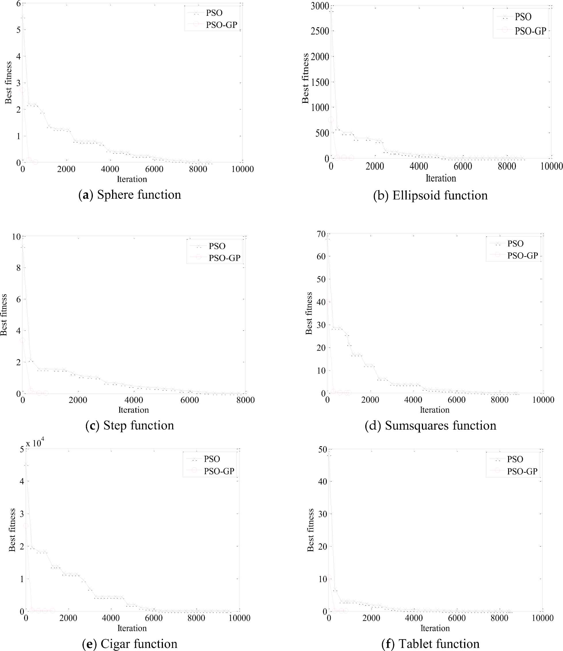
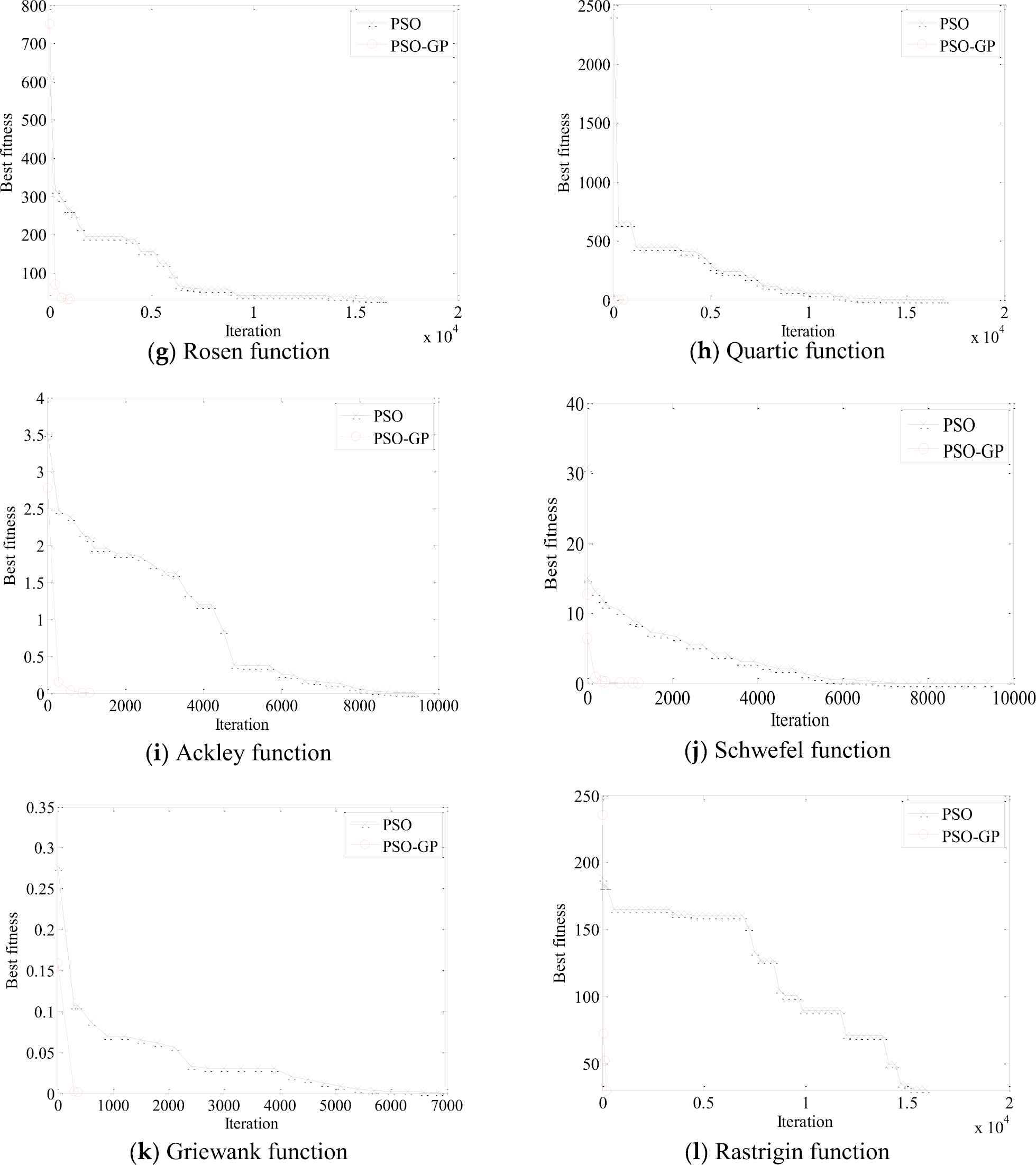
Convergence of the Gaussian process-particle swarm optimization (GP-PSO) algorithm for 30-dimensional benchmark functions.
In addition, both GP-PSO and PSO can achieve expected accuracy (see Table 2) after over 30 times runs for all experiments. It demonstrates that the robustness of GP-PSO is the same as PSO. The robustness of two algorithms is comparable, because the GP-PSO does not change the principle rule of evolution; in our algorithm, we just take advantage of GP to estimate the most potential solution then improve the searching speed of PSO. GP-PSO and PSO have the ability of searching the global optimum, but GP-PSO is more efficient than PSO.
As shown in Figure 3, the converge of GP-PSO is the fastest within iteration of 1000. Therefore, the converge of PSO and GP-PSO with iteration of 300/600/900 in the different 30-dimensional functions were compared in Table 6. The PSO and GP-PSO start to show distinct performance in optimization from iteration of 300. With the increase of iteration, the optimal value decreases for both methods. For iteration of 900, PSO can't meet the requirement of accuracy for all of the functions. GP-PSO associated with Rastrigin function will achieve the accuracy with iteration of 300; for Griewank and Sphere, Step, Tablet, Quartic function, iteration of 600 and 900 are sufficient, respectively. The iteration of residual function is over 900 for both methods.
| Function | 300 |
600 |
900 |
|||
|---|---|---|---|---|---|---|
| PSO | GP-PSO | PSO | GP-PSO | PSO | GP-PSO | |
| Sphere | 2.198442 | 0.087529 | 2.175041 | 0.001023 | 1.911124 | 0.000913 |
| Ellipsoid | 594.628497 | 2.414306 | 493.550394 | 0.156631 | 493.550394 | 0.002018 |
| Step | 2.155441 | 0.176797 | 1.557810 | 0.009128 | 1.523526 | 0.000709 |
| Sumsquares | 28.746118 | 0.587226 | 28.746118 | 0.098386 | 25.947067 | 0.003208 |
| Cigar | 19763.982314 | 247.688017 | 18366.828056 | 5.043769 | 18366.828056 | 0.251856 |
| Tablet | 6.823563 | 0.071880 | 3.118476 | 0.006294 | 3.118476 | 0.000822 |
| Rosen | 317.017070 | 69.640895 | 295.183256 | 35.633361 | 266.358637 | 30.845138 |
| Quartic | 651.919176 | 0.174035 | 651.919176 | 0.086739 | 651.919176 | 0.000736 |
| Ackley | 2.473627 | 0.149701 | 2.381386 | 0.032678 | 2.165373 | 0.006058 |
| Schwefel | 12.146868 | 0.414506 | 10.484639 | 0.076709 | 8.918804 | 0.009359 |
| Griewank | 0.107419 | 0.002093 | 0.087207 | 0.000665 | 0.069805 | 0.000665 |
| Rastrigin | 182.095993 | 29.991134 | 164.769693 | 29.991134 | 164.769693 | 29.991134 |
GP, Gaussian process; PSO, particle swarm optimization.
Comparison of the fitness evaluation between GP-PSO and PSO.
5. CONCLUSIONS AND FUTURE STUDY
It is important to reduce the number of function evaluations when optimizing expensive fitness functions. This can be achieved by exploiting knowledge of past evaluated points to train an empirical model, which can be used as inexpensive surrogate of the fitness function. This paper has shown that the combination of PSO and GP can be used as fitness function surrogates to solve the complex problems of function global optimization. In the proposed algorithm, the GP dramatically reduces the number of function evaluation and provides accurate estimation of the global optimum solution; in addition, the dynamically update training datasets for training GP improves the approximation accuracy of the GP. The results have clearly demonstrated that the proposed algorithm is superior to PSO, which is widely accepted as an efficient tool to solve the very ill-conditioned problems of global optimization. Excellent performance and easy implementation of GP-PSO shows a good potential in computationally expensive optimization problems.
The proposed algorithm is specified for the complex and nonlinear optimization problem in many engineering fields, such as mechanical, civil and aerospace engineering. In most of the cases, the computational cost is extremely high, which can't be afforded by means of conventional algorithm; especially for large-scale finite element analysis or computational fluid dynamics simulations. Furthermore, from the aspect of complexity, it is challenging because many global optimization cases involve objective functions of multimodal, highly nonlinear, with steep and flat regions and irregularities. In this work, though the applicability can't be fully verified, the superiority of proposed algorithm has been proved by comparing with variety of typical standard benchmarks. Moreover, the GP in this algorithm is only based on exponential covariance function. In the future, more covariance functions will be tested; such as Matern covariance function and linear covariance function. Additionally, the performance of the proposed algorithm is only tested with the typical benchmark functions in this work. The expansibility and applicability will be validated by introducing the data from the practical cases. And also, the proposed strategy will be extended in terms of more combinations to form up the new algorithm.
CONFLICT OF INTEREST
The authors declare no conflicts of interest.
AUTHORS' CONTRIBUTIONS
Yan Zhang and Hongyu Li proposed the main idea of the paper, developed and validated the algorithm, and analyzed the results. Enhe Bao and Aiping Yu contributed with the idea to provide the benchmark of the algorithm. Lu Zhang conducted the literature survey and contributed to the introduction section and polished the paper. Yan Zhang, Hongyu Li and Lu Zhang wrote the manuscripts with the support from other co-authors.
ACKNOWLEDGMENT
The present work was supported by the National Natural Science Foundation of China (Grant Nos. 51708147, 51409051 and 51568014), the Natural Science Foundation of Guangxi (Grant Nos. 2017GXNSFBA198184 and 2014GXNSFBA118256), Guangxi Science and Technology Base and Special Fund for Talents Program (Grant No. Guike AD19110044) and Guangxi Innovation Driven Development Project (Science and Technology Major Project, Grant No. Guike AA18118008). The authors also would like to thank the partial support from Guangxi Key Laboratory of Geomechanics and Geotechnical Engineering (Grant Nos. 14-B-01 and 2015-A-01-05).
REFERENCES
Cite this article
TY  - JOUR
AU  - Yan Zhang
AU  - Hongyu Li
AU  - Enhe Bao
AU  - Lu Zhang
AU  - Aiping Yu
PY  - 2019
DA  - 2019/11/12
TI  - A Hybrid Global Optimization Algorithm Based on Particle Swarm Optimization and Gaussian Process
JO  - International Journal of Computational Intelligence Systems
SP  - 1270
EP  - 1281
VL  - 12
IS  - 2
SN  - 1875-6883
UR  - https://doi.org/10.2991/ijcis.d.191101.004
DO  - 10.2991/ijcis.d.191101.004
ID  - Zhang2019
ER  -