
Hybrid Dragonfly Optimization-Based Artificial Neural Network for the Recognition of Epilepsy
- DOI
- 10.2991/ijcis.d.191022.001How to use a DOI?
- Keywords
- Electroencephalography; Kalman filter; Variable mode decomposition; Modified principal component analysis; Artificial neural network; Hybrid dragonfly algorithm
- Abstract
Epilepsy can well be stated as a disorder of the central nervous systems (CNS) that brought about recurring seizures owing to chronic abnormal blasts of electrical discharge on the brain. Knowing if an individual is having a seizure and diagnosing the seizure type or epilepsy syndrome could be hard. Many methods were developed to recognize this disease. But the existing techniques for detection of epilepsy are not satisfied with accuracy, and cannot identify the diseases effectively. To trounce these drawbacks, this paper proposes an approach for the recognition of Epilepsy as of the electroencephalography (EEG) signals. This is implemented as follows. Primarily, the Kalman filter (KF) is utilized for pre-processing to eradicate the impulse noise present in the EEG signals. This filtered signal is then decomposed utilizing variable modes decomposition (VMD). Feature extraction (FE) is performed by computing 7 features. The dimensionality of this signal is then lessened using Modified-Principal Components Analysis (M-PCA). Finally, classification is conducted utilizing the artificial neural networks (ANN) that is optimized using the hybrid dragonfly algorithm (HDA). Disparate performance metrics such as sensitivity, accuracy, and false discovery rates (FDR) are ascertained and as well weighted against with the existent works.
- Copyright
- © 2019 The Authors. Published by Atlantis Press SARL.
- Open Access
- This is an open access article distributed under the CC BY-NC 4.0 license (http://creativecommons.org/licenses/by-nc/4.0/).
1. INTRODUCTION
The word “Epilepsy” is the rifest neurological disorders in human. Epilepsy is found to affect numerous patients all through the earth [1–3]. This disorder is a member of the shortcoming in the central nervous systems (CNS) which has consequences like recurring, un-provoked epileptic seizures owing to chronic abnormal blasts of electrical discharge [4].
There are circumstances when patients might not be conscious that they are a prey to seizures owing to the random nature of its occurrence. Such seizures are detected by the brain's electrical action [5–7]. The electrical action of a normal brain is much different from the electrical action of epilepsy affected persons.
It is monitored by utilizing the electroencephalography (EEG) [8–10]. It stands as a non-invasive system that gauges the voltage fluctuations resultant from the ionic current in the brain neurons. These signals can well be employed as an instrument to identify epilepsy as it brings abnormalities on the readings. Various variations on the EEG signal imply the occurrence of an abnormality in that particular individual.
The disparate stages of this disorder can as well be detected. It is employed to identify the preictal step that is the stage earlier than the actual seizure happens. This stage remains for fewer minutes to over a day. The subsequent stage is the ictal [11] stage that is when the seizure occurs. The tertiary stage is postictal stage [12–14] that is the stage subsequent to the seizure has seized. The stage betwixt the postictal and preictal stage is termed interictal stage [15]. This paper tackles an automatic and accurate methodology aimed at diagnosing epilepsy utilizing EEG signals.
The remaining section of the paper is pre-arranged as; Section 2 tackles the review of the associated works. Section 3 detailed the techniques involved in the proposed method, Section 4 gives the experimental outcomes and also Section 5 deduces the paper.
2. RELATED WORKS
Numerous existing works are associated to the epilepsy detection utilizing EEG signals. A few works are detailed in this section.
Alickovic et al. [16] suggested a prototype for the automatic seizures detection & prediction by utilizing the EEG signals. The signals as of 2 databases were processed. This model was defined utilizing four components. The preliminary component was the multi-scaled principal component analysis (PCA) for de-noising the signal. Signal decomposition (SD) was the second component. Then, the statistical traits of the relevant features were obtained and the fourth component was the employment of machines learning algorithm.
Fan and Chou [17] presented an investigation on the spatial temporary synchronizations pattern on epileptic brains utilizing the spectral graphs theoretic features. A statistic control chart was implemented for the extorted features over time for scrutinizing the transits as of the normal to the epileptic states in multi-vibrate EEG. This approach validated the increased temporal synchronization in epileptic EEG.
Mert and Akan [18] suggest a multivariate extension (ME) centered feature extortion technique. This was performed for processing the multichannel EEG signals aimed at emotion recognition. The multi-channels intrinsic modes functions that were extorted by the ME were analyzed utilizing disparate time and also frequency domain methodologies. This methodology was implemented for an EEG dataset together with its outcomes were contrasted with existent works.
Gupta et al. [19] developed the automatic seizures detection framework on EEG signals. A multi-rate structure was constructed centered on the vectors of the DCT (discrete cosines transform). The signal was disintegrated into theta, alpha, delta, and also gamma waves. These waves were modeled statistically using the “fractional Brownian motion” together with the “fractional Gaussian noises.” The Hurst exponents value together with auto-aggressive moving averages parameters was utilized as features for the binary “support vector machine” (SVM).
Tiwari et al. [20] formulated a means for the EEG based epilepsy diagnosis. This method involved the finding of the vital points in at the manifold scales in the signals of EEG. This was done utilizing a pyramid of disparity of the Gaussian filtered signals. The local binary patters were computed at the vital points. The histogram of these patterns was regarded as the characteristic set. This is fed to the SVM intended for the EEG signals' classification.
Patidar and Panigrahi [21] prepared a diagnostic approach meant for the examination & classification of seizure and seizure-free EEG signals. This method began with the application of the “tunable-Q wavelet transform.” This decomposed the signals in to sub bands for good feature extraction. The kraskovs entropy was computed so as to discriminate the seizure-free signals as of the epileptic seizures EEG signals. The classification was done using the least squares “SVM” classifier.
Zhang and Chen [22] developed a times-frequency analytical algorithm called local means decomposition. Initially, the signal was decomposed in to a sequence of product functions. After that, the temporal statistical and also non-linear aspects of the first five product functions were calculated. The features were inputted to 5 classes namely; “backpropagation neural network” (BPNN), “k-nearest neighbor” (KNN), “linear discriminant analysis” (LDA), “un-optimized SVM,” and SVM optimized utilizing “genetic algorithm” (GA-SVM).
Vidyaratne and Iftekharuddin [23] recommended a method aimed at the automatic finding of the epileptic seizure using the scalp along with the intracranial EEG. This technique obtained a harmonic multi-resolution and also self-similarity centered fractal features using EEG. The harmonics wavelet packets transform was computed centered on the Fourier transforms. Fractal dimension was attained to capture the self-similar recurring patterns on the EEG signal. The energy features at every epoch were organized. The last feature vector combined the feature configurations of every epoch within the particular moving window to reflect the EEG temporal information. The significance vector machine used to categories the features vectors.
Parvez and Paul [24] put forth a seizure prediction method centered on the spatiotemporal relationship of the EEG using phase correlation. This technique measured the relative change betwixt the current & reference vectors of EEG signals. This can well be utilized to spot the sort of EEG and also encompass the capability to forecast the seizure. This method was less responsive to artifacts.
3. PROPOSED SYSTEM
The proposed work is executed in 5 distinct stages. The preliminary one is the pre-processing stage. This stage is implemented to eradicate unwanted signals that exist on the EEG signal. The next stage is the SD. This process is conducted utilizing the VMD. The decomposed signal undergoes feature extraction. In this stage, seven relevant features are extorted as of the decomposed EEG signal. The features that are extorted are wavelet entropy (WE), root mean squares (RMS), means, standard deviation (SD), Hurst exponent, skewness, and also kurtosis. Then, the dimensionalities of the traits that are extracted are reduced. This is done utilizing M-PCA. Finally, the EEG signals are categorized utilizing an optimized ANN. The optimizations algorithm that is used in the proposed work is the hybrid dragonfly algorithm (HDA).
Consider a database
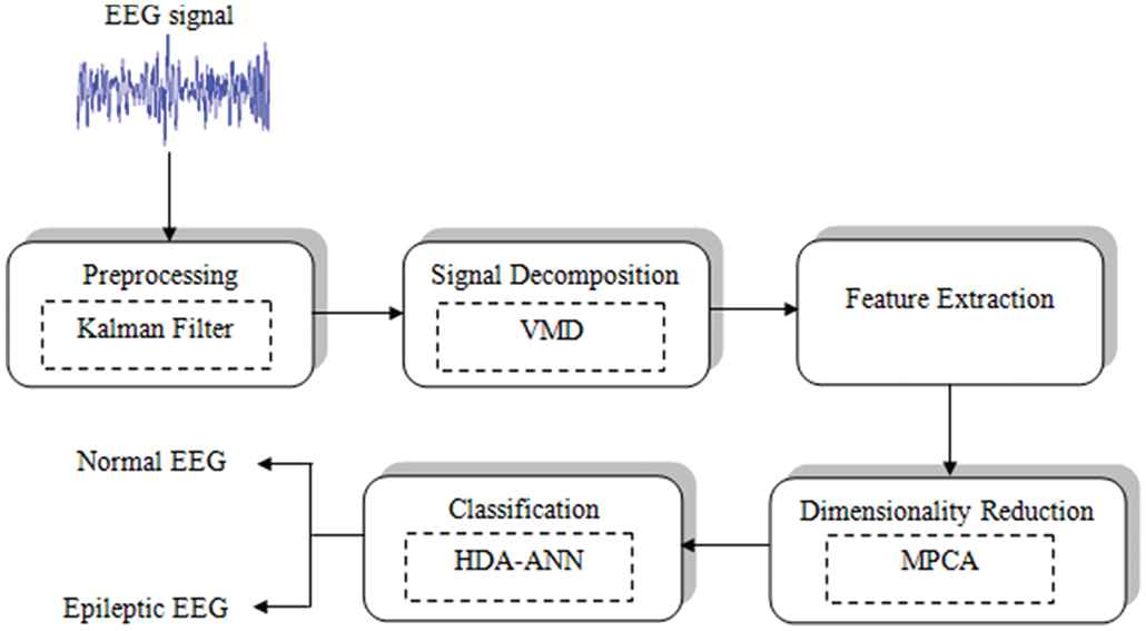
Block diagram of the proposed system.
3.1. Pre-processing
The EEG signals emanate from the brain. These impulses can well be infected with noise that requires to be filtered to attain the actual brain signal. Here, the EEG signals are filtered by utilizing the “Kalman filter.” This filter stands as a group of mathematical equations which provide an effectual computational means to evaluate the process condition by minimizing errors.
This filter encompasses the capability to make more reliable estimates for a sequence of observed measurements. The steps comprised in this filter are as follows. A forecast of the state is done centered on the previous values together with the model. The measurement from the signal is then obtained. This is followed by the process of updation based on errors. This entire process is then repeated.
The Kalmans gain stands as an important element of the Kalmans filter. This is centered on the error that occurs in the preceding estimation. For a good predication, the Kalmans gain functions to cancel the new measurements. The signals are regarded as states and new states are calculated centered on the preceding states. The Kalmans gain is computed as of the novel state. The current assessment that is obtained as denoted in the Equation (1).
Where,
3.2. Signal Decomposition
The subsequent phase of the proposed work is SD. Here, the filtered signal gets decomposed. It targeted to isolate the signal elements as of the composite signals. In the proposed system, SD is performed utilizing a methodology termed VMD. VMD is utilized for decomposing an input signal to a discrete number of modes (sub-signals) that has certain sparsity properties while regenerating the input. The sparsity subsequent to every mode is selected to be its bandwidth on spectral domain. The narrow-band signal or narrow-band mode function is denoted as
Where, phase change
The complex signals is usually decomposed to discrete
Where, the number of modes
3.3. Feature Extraction
The 3rd phase in the proposed system implementation is the process of extorting the features that delineate the EEG signal characteristics. A total of 7 features are concurrently extracted. The decomposed ECG signal
3.3.1. Wavelet entropy
The primary feature that is extorted in this proposed system is the WE feature. WE are a new effectual tool with the competency to discover the signals' transient features. The dynamics of EEG results are determined to utilize this feature. WE is a time function and is scientifically represented as in the Equation (5).
Where,
3.3.2. Root mean square
The secondary feature that is extorted in the proposed system is the RMS. The robustness of an EEG signal is taken as of the signal to gauge the potency of every EEG sample data. This is performed by computing the RMS value. RMS is the quadratic means which is helpful when positive together with negative variations are found on a signal. This feature is evaluated on the frequency domains as in the formula.
Where,
3.3.3. Mean
The signal of ECG comprises disparate peaks. The mean for signal values is evaluated as a parameter that is extorted as a characteristic feature. This feature has a distinctive range not only for the normal signals but also for the signals that are affected by the epileptic seizures. The subsequent equation provides the mathematical depiction of mean calculation.
Where,
3.3.4. Standard deviation
It is utilized to gauge the degree of variations in the collection of data values. It is as well termed as RMS deviation as it is the squares roots of the average values of the pre-squared deviations as of the arithmetical means. Its computation formula is,
Where,
3.3.5. Hurst exponent
The subsequent feature that is extorted for the pre-decomposed signal is the Hurst Exponents. This is gauge of predictability, self-similarity, and the level of longest-range reliance in a time series. It is similarly a gauge of the smoothness of a fractal time-series grounded on the asymptotic conduct of the re-scaled gamut of the procedure in line with the Hurst's summed up the time series equation. This is mathematically depicted as,
Where,
3.3.6. Skewness
The subsequent feature that is extorted as of the EEG signal is skewness. It is a standardized instant of an arbitrary signal. It delineates the asymmetry in distribution about the median. It is positive/negative contingent on the signal. It is mathematically delineated as,
3.3.7. Kurtosis
It gauges whether the provided data is flat relative or peaked in normal distributions. That is, the dataset which has a higher kurtosis shows a distinctive peak nearer to the median. They decrease quickly and have hefty tails. Datasets with low kurtosis normally possess a flat top nearer to the median in the place of a pointed peak. Kurtosis ascertains the intensity of random variable distribution. The mathematical delineation of Kurtosis is,
3.4. Reduction of Dimensionality
The process of lessening the dimensionality of the feature space with considerations by attaining a pool of principal features is termed as dimensionality reduction. It lessens the storage space as well as the time required. Removal of multi-collinearity ameliorates the interpretation of the parameters of the proposed model and also it becomes easy in visualizing the data when lessened to extremely low dimensions. Here, the process of dimensionality reduction is done with the help of M-PCA.
3.4.1. Modified-principal component analysis
PCA is an eminent method for diminishing the signal dimensionality; therefore, it is utilized for classification. It attains a linear mapping of a higher to a low dimension input vector. It also attains a distinctive solution by compelling a particular orthogonal structure to the mapping matrix. The PCA evaluates the principal elements as a percent of the entire changeability of the data.
The decomposition of a multichannel signal like EEG signals generates separate signals of a solitary channel for the extortion of valuable information. PCA is utilized to execute feature extortion utilizing linear algebra results to diminish the signal dimension in matrix form
Feature transformation needs the assessment of the data on the covariance matrix, its eigen value- eigen vector decomposition and as well the storage of those values in lessening order. Then, the data is presented to the novel subspace delineated by the principal elements.
Here, an M-PCA is employed for feature reduction. This has a slighter difference as of the PCA. The Gaussian kernel is employed in the preliminary step of M-PCA. Gaussian kernel utilizes a measure of the similarity betwixt points for predicting the feature value. Besides an estimate for that feature, this prediction also gives uncertainty information. It is as well termed as one-dimensional Gaussian distribution. Subsequently, the covariance matrix is evaluated and its eigen values are assessed. Those are next translated to corresponding principal elements. This is implied as
Step 1: A Gaussian kernel is used to the features that are extorted.
Step 2: Thereafter, the covariance matrix is evaluated.
Step 3: The Eigen vectors of the covariance vectors are calculated.
Step 4: Those data are then translated to components that could augment further processing.
3.5. Classification
The last step of the proposed system is the classification. The output of M-PCA (reduced features) is given to the HDA-ANN classifier. In this, the weight values of ANN are optimized using HDA to categorize the signals as epileptic and normal signals.
3.5.1. Artificial neural network
Here, the HAD-ANN classifier is utilized for classification purpose. In this, the reduced features are inputted into ANN. Then the weights in ANN are optimized using HAD. So the classification model is named HAD-ANN. The steps of ANN and HAD is explained below.
The ANN stands as a mathematical form which is emboldened by the biological NN. This model contains several inter-connected artificial neuron. These are formed of several interconnections associated with adaptable weights. The general composition of a neuron contains a layer of input, output, and also a minimum of one hidden layers. This approach has seen a wide usage in different classification applications. In an ANN, the decision making procedure is generally considered as a holistic approach. It is purely centered upon the features of the input patterns that are appropriate for the medical data classification.
The reduced features that are obtained from the preceding process of the proposed work are classified centered on their individual characteristics into 2 separate classes named namely i) normal EEG ii) Epileptic EEG signal. The architecture of the ANN that is used on the proposed work is displayed in Figure 2.
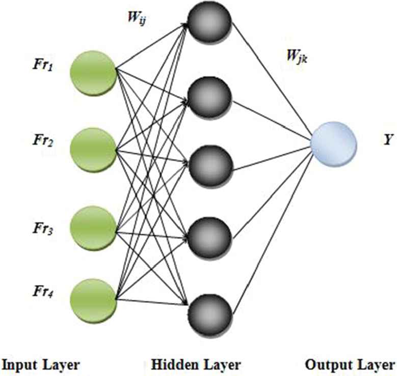
General structure of artificial neural networks (ANN).
The sort of ANN used is the BPNN. The ANN algorithm is illustrated below.
Step 1: Initialize all the weights which are needed for the functioning of the algorithm.
Step 2: For each set of input vector, carry out 3–5 steps.
Step 3: For
Step 4: For
Where,
Step 5: For
Where,
Step 6: Determine the output's error function using the subsequent equation.
Where,
3.5.2. Hybrid dragonfly algorithm
The chief goal of any swarm is survival. To achieve this objective, all the individuals must be paying attention toward food sources and also distracted toward enemies. These are modeled mathematically. The proposed work employs a hybrid edition of the conventional dragonfly algorithms. The two algorithms that are merged are the GA and the dragonfly algorithm. The steps involved in the HDA are explained below.
Step 1: Initializations of the populace and the step vector and formulate the objectives function.
Step 2: Evaluate the values of
Where
Alignment indicates the velocity corresponding of individuals with that of the other individuals on the neighborhood. Alignment is computed as below.
Where
Cohesion refers to the inclination of individuals toward the middle of the mass of the neighborhood. The cohesion is computed as follows.
The attraction for a food source is computed as below.
In which,
The Distraction toward and enemy is formulated as shown here.
Where,
Step 3: To up-date the dragonflies position on a search space and also simulate their movements, 2 vectors are needed that is the step and position vector. The step vector indicates the direction of the dragonfly's movement furthermore is represented as given here.
Where
Step 4: The positions vector can well be computed from the step vector value. It is calculated as follows.
Where
Step 5: The positions of the dragonfly is updated utilizing the subsequent equation.
In which,
Step 6: If the stop criteria are unsatisfied, then two genetic operators are added. Crossover and mutation are applied when the dragonfly doesn't have as a minimal of one neighboring dragonfly. This makes the optimization more effective. The sort of crossover that is used is the 2 point crossover. This is done using the crossover points.
Where
Step 7: Mutation is performed by replacing several genes from each chromosome with new genes. The swapped genes are arbitrarily generated genes without any repetition inside the chromosome. Here, the chromosomes are the collection of parameters that define the solution. The proposed algorithm's flowchart is displayed in Figure 3.
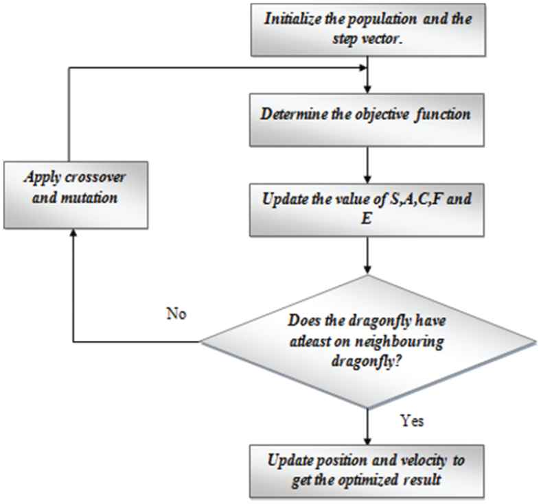
Workflow of the hybrid dragonfly algorithm (HAD).
4. EXPERIMENTAL RESULTS
This proposed method for the recognition of Epilepsy is implemented in the MATLAB (version 14) platform with the machine configuration:
Processor: Intel core i7
CPU Speed: 3.20 GHz
OS: Windows 7, RAM: 4GB
4.1. Database Description
The database used in the proposed work was an openly available open source database called the CHB-MIT database. This database was gathered at the Children's Hospital, Boston. The database holds EEG recordings as of different pediatrics subjects with in-tractable seizures.
The subjects were perceived for numerous days following removal of antiseizure medication so as to differentiate their seizures, additionally, evaluate their candidacy for surgical interference. The “EEG recordings” were gathered as of an aggregate of twenty-two subjects. Among these 22 subjects, 5 were males in the range of 3–22 and 17 were females in the age set of 1.5–19. All the signals in this database were sampled at 256 samples/second with 16 bit resolution. 22 epileptic signals and 8 normal EEG were considered for the training the proposed work.
4.2. Performance Analysis
This is done using different performance metrical. To evaluate these parameters, 4 basic metrics should be calculated. They are the “true positive” (TP), “false positive” (FP), “true negative” (TN), together with the “false negative” (FN) values. The values of TP denote the situation wherein epilepsy is present and it is detected. TN represents the condition in which the EEG signal belongs to a healthy individual and it is detected as a health EEG signal. FP indicates the healthy EEG signals that are falsely classified as epileptic signals. FN refers to the EEG that is correctly classified as normal signals.
The “positives predictive values” (PPV) along with the negatives predictive values (NPV) is the proportions of the positive in addition to the negative outcomes respectively. These are statistical measures that play an imperative part in estimating the proposed system's performance. The mathematical representations of the PPV along with the NPV are as follows.
Sensitivity is a statistical measure of performance. It is as well called TP rate. It gauges the actual positives' proportion that is correctly identified in each situation. Accuracy determines how correctly the signals are classified. Markedness stands as the state of standing out as odd in contrast to a more common/regular form. The mathematical illustrations of these 3 parameters are below.
False discovery rates (FDR), as well as false omission rate, is the two other measures of performance that are determined for the proposed system. These are values are computed employing the subsequent relations.
Table 1 displays the performance parameters that are estimated for the proposed system.
| Parameter | Value |
|---|---|
| PPV | 0.9545 |
| NPV | 1 |
| Sensitivity | 1 |
| Accuracy | 0.9667 |
| Markedness | 0.9545 |
| False discovery rate | 0.0455 |
| False omission rate | 0 |
NPV = negatives predictive values, PPV = positives predictive values
Performance metrics of the proposed system.
4.3. Comparative Analysis for Different SD Techniques
The existing SD approaches, like, empirical modes decomposition (EMD) along with Continuous Wavelet Transformation are contrasted with the proposed VMD procedure using performance metrics say accuracy and sensitivity. The following graph shows these approaches' comparison.
In terms of accuracy, the proposed VMD shows an elevated performance that is 0.9667. The incessant wavelet transform yields the least value of accuracy that is 0.8775. From Figure 4, it can be noted that the proposed work encompasses better values of accuracy and sensitivity when contrasted to the values that were attained from the existent systems like the EMD together with the incessant wavelet transformations.
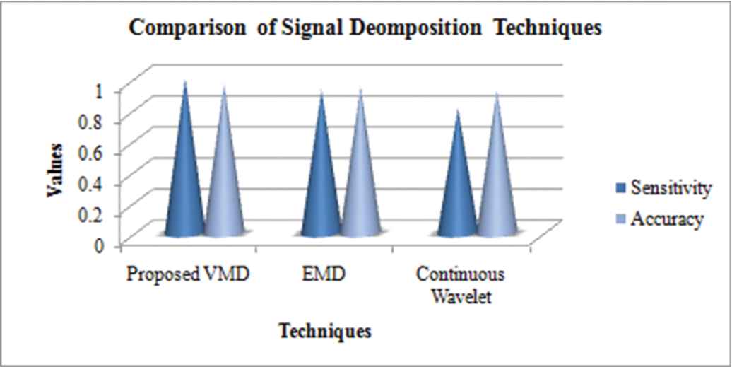
Signal decomposition analysis.
4.4. Comparative Analysis for Different Classifiers
The function of the classifier is crucial to the proposed system. The classifier performs the categorization of the EEG into specific classes centered on the features which are extracted as of the signal. The “False Negative Rates” (FNR) together with the accuracy is chosen as the performance metrics to determine the efficiency of the proposed classifier along with other existent classifiers. The equation for calculating FNR is below.
The following table depicts the values of FNR along with its corresponding accuracy for the proposed HDA-ANN and other existing classifiers. The classifiers that are taken for the comparative analysis are the ANN, General Regression-NN (GRNN), K-nearest neighbors (KNN), and nearest neighbors (NN).
The below Table 2 depicts the values of FNR along with its corresponding accuracy for the proposed HDA-ANN and other existing classifiers. The ANN gives good results (accuracy = 0.956, FNR = 0.07) among existing classifiers. But the proposed HAD-ANN classifier gives superior outcomes (accuracy = 0.9667, FNR = 0) when compared to others.
| Classifiers | FNR | Accuracy |
|---|---|---|
| HDA-ANN | 0 | 0.9667 |
| ANN | 0.07 | 0.956 |
| GRNN | 0.13 | 0.8620 |
| KNN | 0.107 | 0.8918 |
| NN | 0.285 | 0.7235 |
ANN = artificial neural networks, FNR = false negative rates, GRNN = general regression nearest neighbors, HAD = hybrid dragonfly algorithm, KNN = K-nearest neighbors, NN = nearest neighbors
FNR and Aaccuracy of different classifiers.
The graphical illustration of Table 2 is displayed in Figures 5 and 6 in terms of FNR and accuracy.
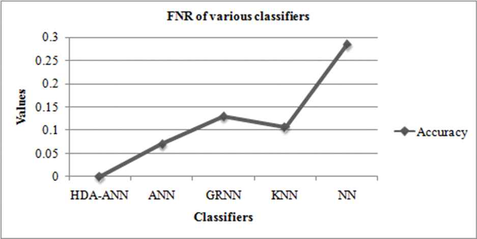
Graph depicting the false negative rates (FNR) of various classifiers.
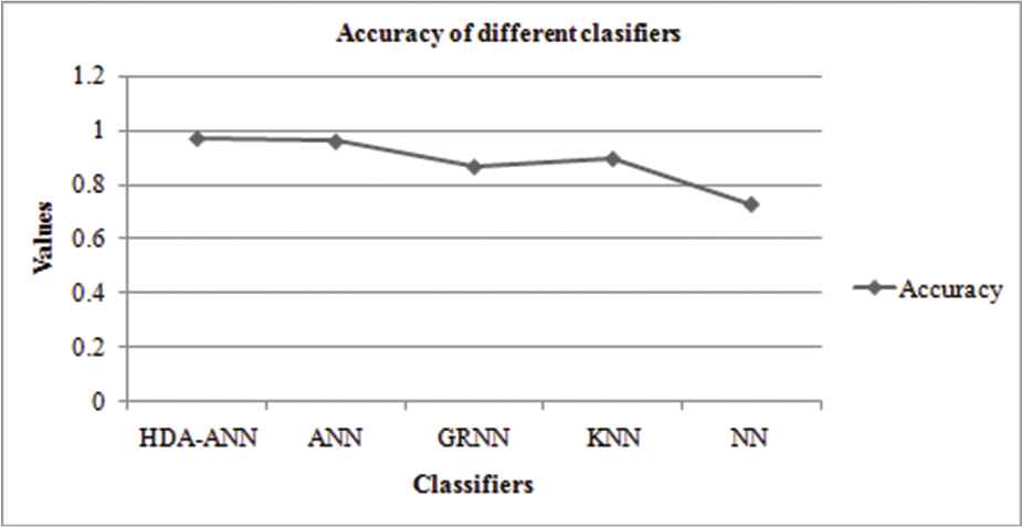
Graph showing the accuracy of various classifiers.
From Figure 5, the FNR (0.285) is seen to be the highest for the NN and also the lowest for the proposed HAD-ANN (FNR = 0) system. So as to attain correct classification results, the FNR values must be low. The accuracy of HAD-ANN and existing methods are compared and shown in Figure 6.
From the above graph, the accuracies of the ANN (0.956), GRNN (0.8620), KNN (0.8918), and NN (0.7235) together with the proposed HAD-ANN (0.9667) classifiers are shown. The proposed work encompasses an effective classifier and can well be utilized in the accurate detection of epilepsy. The NN performance is poor on considering the other classifiers.
5. CONCLUSION
This paper undertakes the epilepsy detection by examining the EEG signal of a person. This signal undergoes pre-processing, SD, feature extractions, dimensionality reduction along with classification. Various performances metrical were computed and evaluated. From the investigational results, the usage of HDA-ANN is justified as it provides promising results when compared to the other existing classifiers. In the future, this system can well be further extended via incorporating some advanced methodologies or algorithms in dimensionality reduction, decomposition, and also in classification which can provide grading of the EEG signals to provide details about disparate stages of epilepsy.
CONFLICT OF INTEREST
The authors declare no conflict of interest.
Funding Statement
There is no Funding for this manuscript.
AUTHORS' CONTRIBUTIONS
All authors contributed equally to the publication of this article with regard to the design of the target model, validation of the numerical model, parametric study, analysis and writing.
REFERENCES
Cite this article
TY  - JOUR
AU  - K. G. Parthiban
AU  - S. Vijayachitra
AU  - R. Dhanapal
PY  - 2019
DA  - 2019/11/15
TI  - Hybrid Dragonfly Optimization-Based Artificial Neural Network for the Recognition of Epilepsy
JO  - International Journal of Computational Intelligence Systems
SP  - 1261
EP  - 1269
VL  - 12
IS  - 2
SN  - 1875-6883
UR  - https://doi.org/10.2991/ijcis.d.191022.001
DO  - 10.2991/ijcis.d.191022.001
ID  - Parthiban2019
ER  -