
Building an Artificial Neural Network with Backpropagation Algorithm to Determine Teacher Engagement Based on the Indonesian Teacher Engagement Index and Presenting the Data in a Web-Based GIS
- DOI
- 10.2991/ijcis.d.191101.003How to use a DOI?
- Keywords
- Artificial neural networks; Backpropagation; Stochastic learning; Steepest gradient descent; Indonesian Teacher Engagement Index; Executive information system
- Abstract
Teacher engagement is a newly-emerged concept in the field of Indonesian teacher education. To support this concept, we designed an artificial neural network (ANN) using backpropagation, stochastic learning, and steepest gradient descent algorithms to determine teacher engagement based on the Indonesian Teacher Engagement Index (ITEI). The resulting ANN may be used in a data-gathering website for teachers to use for self-evaluation and self-intervention. The optimal architecture for the ANN has 44 input nodes, 26 first hidden layer nodes, 20 second hidden layer nodes, and 7 output nodes, with a learning rate of 0.05 and trained over 5000 iterations. The sample data used for training was gathered by ITEI researchers and the Executive Board of Indonesian Teachers Association (Pengurus Besar Persatuan Guru Republik Indonesia, PB-PGRI) and includes data of teachers from all around Indonesia. The maximum accuracy of this ANN was 97.98%. The sample data were then used to create an executive information system presented in the form of a map created using ArcGIS Pro software.
- Copyright
- © 2019 The Authors. Published by Atlantis Press SARL.
- Open Access
- This is an open access article distributed under the CC BY-NC 4.0 license (http://creativecommons.org/licenses/by-nc/4.0/).
1. INTRODUCTION
The government of Indonesia supervises teacher competence and performance based on pedagogic competence, personality competence, social competence, and professional competence through a teacher certification program [1]. But teachers should also be engaged in their profession, not only competent and performing. To evaluate the level of teacher engagement that the teacher has, a tool called the Indonesian Teacher Engagement Index (ITEI) was developed.
ITEI is based on the concept of engagement in the context of education to complement the performance instruments that have been made by the Indonesian government. A teacher in Indonesia in carrying out his profession will produce optimal performance when the teacher has a positive psychological condition so that he can form a positive educational culture. Teachers are also expected to have basic competencies according to government standards and apply values in accordance with the basic philosophy of the Indonesian state and be able to apply nationalism leadership engagement in carrying out their profession. [2]. The ITEI has 6 dimensions. These dimensions are expressed in 22 indicators, with every indicator having 2 statements each, totaling 44 statements. For evaluation, the teacher is given a questionnaire with these 44 statements, to which he or she should express agreement on according to the Likert scale [3]. From these statements, the ITEI score can be determined. ITEI has 7 levels of scoring, from 1 (Disengagement), 2 (Frustrated), 3 (Burn Out), 4 (Dependent Engagement), 5 (Self-Interest Engagement), 6 (Critical Engagement), and finally 7 (Full Engagement). The data gathered by ITEI researchers and the Executive Board of Indonesian Teachers Association (Pengurus Besar Persatuan Guru Republik Indonesia, PB-PGRI) includes data of teachers from all around Indonesia and can potentially be categorized as big data in the future. Big data itself is characterized by high volume, velocity, and variety [4].
In addition, an executive information system is needed to present teacher engagement diagnosis in a district level, as intervention should not be top-to-bottom (from central government to district) nor bottom-to-top (from district to central government); instead, it should be in context for each district. Hopefully, with this executive system, context-based intervention based on the diagnosis is possible.
2. RELATED WORKS
The ITEI was developed since 2015 through a grant by the Indonesian Ministry of Research and Higher Education (Kementerian Riset dan Pendidikan Tinggi, Kemenristekdikti) partnered with the Directorate General of Teachers and Educational Manpower (Direktorat Jenderal Guru dan Tenaga Kependidikan), the Indonesian Ministry of Education and Culture (Kementerian Pendidikan dan Kebudayaan Republik Indonesia), and the Executive Board of Indonesian Teachers Association (Pengurus Besar Persatuan Guru Republik Indonesia, PB-PGRI). A few applications were developed to facilitate data gathering and engagement evaluation of Indonesian teachers, such as a mobile application [5] and a website, http://www.itei.me. The teacher engagement data gathered by ITEI researchers and PB-PGRI on teachers from various regions around Indonesia has reached 10,642 validated data and around 2,000 unvalidated data. If the ITEI system is officially implemented, it may reach the status of big data due to its volume, containing millions of data of teachers from all regions of Indonesia. Big data has an important role in education, especially in teacher evaluation. It brings objectivity to the subjective and intuition-based work that is teacher evaluation [6].
While the aforementioned website uses an artificial neural network (ANN) to predict the ITEI score of a teacher, the development of the ANN used the deep learning libraries Keras and Tensorflow, resulting in an ANN with an accuracy of 97.65%. In this research, we aim to develop a more accurate ANN using the backpropagation, stochastic learning, and gradient descent algorithms [7] using less powerful libraries [9–11].
3. METHODS
3.1. System Architecture and Dataset
In building the ANN, the learning method used was supervised stochastic learning with backpropagation and steepest gradient descent algorithm, with 80% training set and 20% test set from 10,642 sample data which represent most of the regions in Indonesia.
The architecture of the ANN is as shown in Figure 1, and the algorithm flowchart is as shown in Figure 2:
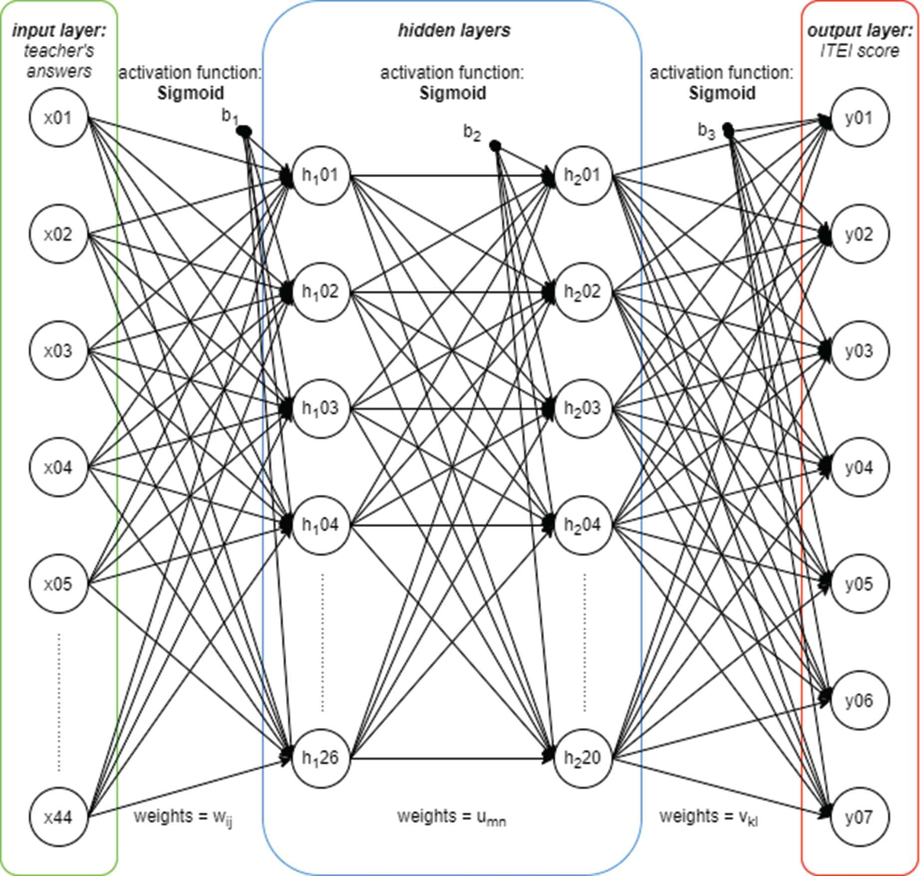
Structure of the artificial neural network (ANN).
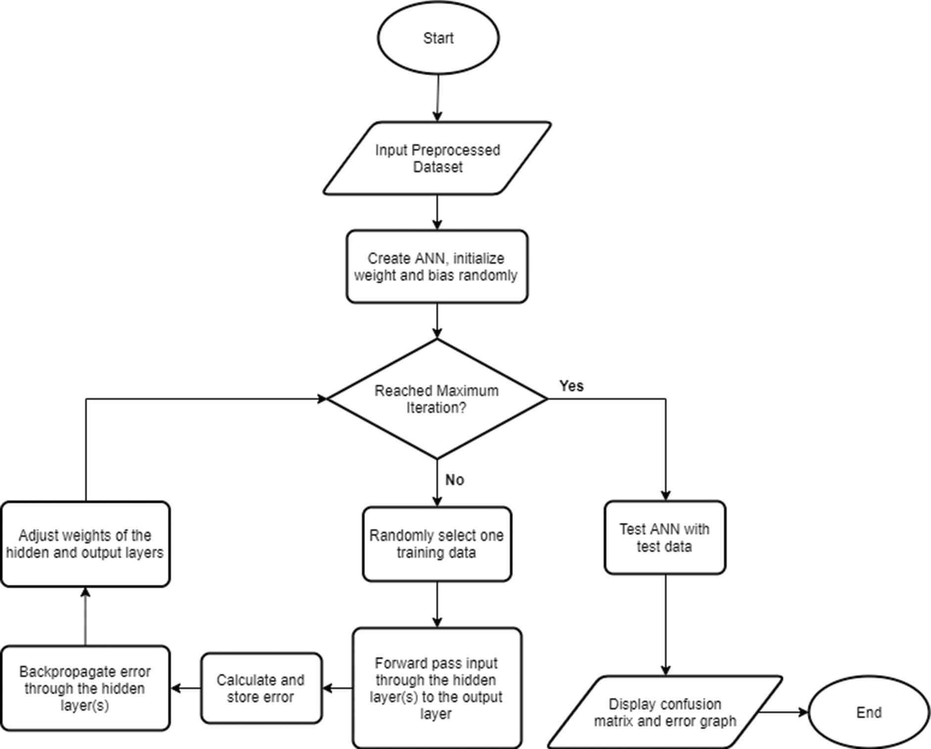
Flowchart of stochastic learning with backpropagation algorithm.
The dataset used was comprised of 1 ID field, 12 demographical fields, 44 questionnaire answer fields, and 1 label field. The 44 answer fields became the input for the ANN, while the label field became the target output. The label field was one-hot encoded before being fed into the ANN, because the resulting output using the sigmoid activation function was an array of values between 0 and 1. To evaluate the accuracy of the ANN, the test set was fed into the ANN and its output compared with the actual labels, resulting in a confusion matrix.
The equations used in feedforwarding and backpropagation is shown below:
Linear combinations:
Sigmoid activation function:
Mean squared error:
Steepest gradient descent:
Chain rule for the second hidden layer → output weights (v):
Chain rule for the first hidden layer → second hidden layer weights (u):
Chain rule for the input layer → first hidden layer weights (w):
3.2. Data Presentation
The dataset containing the sample data was processed manually in Microsoft Excel using PivotTable to convert its individual primary key into regional primary key. The processed table was then imported into ArcGIS Pro and joined as attributes with a Shapefile table containing spatial data of Indonesian districts. The average of ITEI score for each district was then calculated and visualized in a GIS map layer.
4. RESULTS AND DISCUSSIONS
4.1. ANN with Backpropagation and Steepest Gradient Descent Algorithm
4.1.1. Initial architecture (44 input nodes, 26 hidden nodes, and 7 output nodes)
First, the ANN algorithm was tested without bias update and with the weights initialized randomly between values 0 to 1 using the NumPy function random.rand(). The initial architecture used was 44 input nodes, 26 hidden nodes, and 7 output nodes. This configuration yielded the results described in the darker bar of Figure 3 (LR = Learning Rate). As we can see, the resulting accuracy was unstable. We then added the bias update code, which improved the accuracy by a significant amount, as seen in the lighter bar of Figure 3.
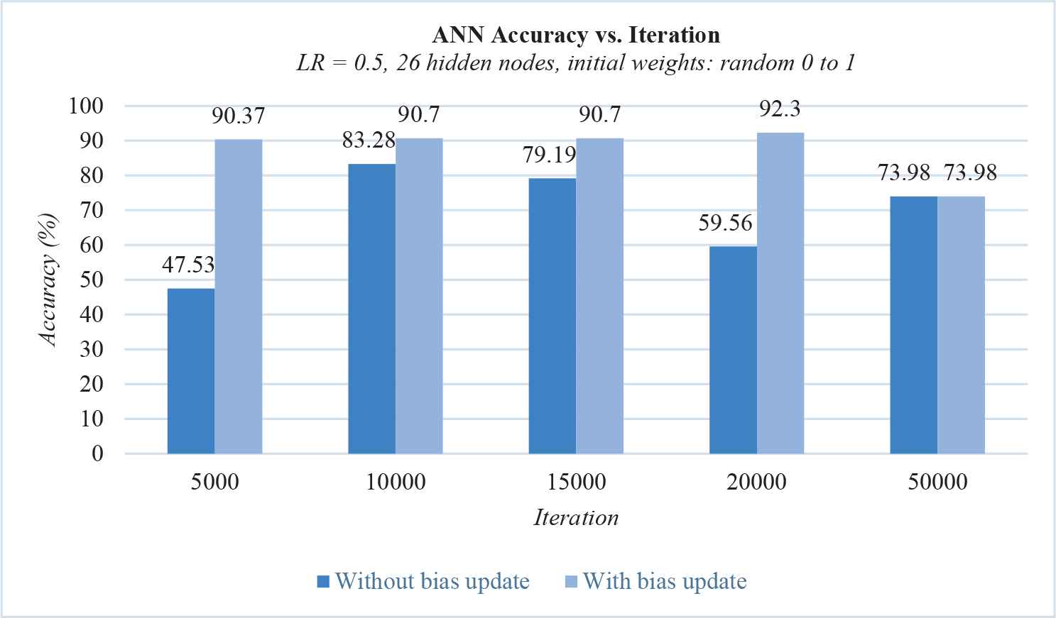
The accuracy of backpropagation gradient descent.
Following the results above, we tried to use the NumPy function random.randn() to initialize the weights to a random Gaussian distribution of mean 0 and variance 1 [8] in order to improve the accuracy. Using this function yielded much better results with only a fraction of iterations than in the previous experiments, as can be seen in Figure 4.
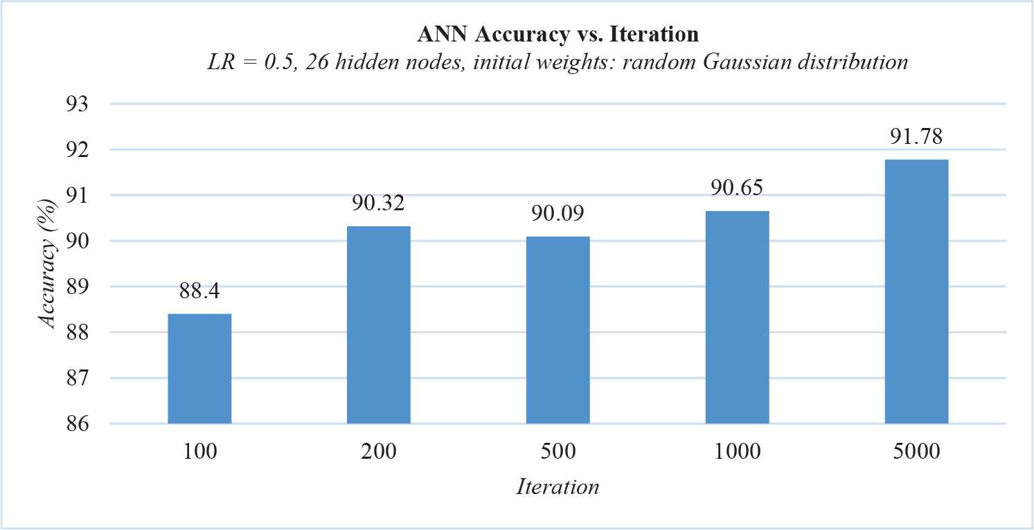
The accuracy of backpropagation gradient descent with initial weights of random Gaussian distribution.
4.1.2. Testing various hidden layer architectures
By this point, the accuracy is already decent, so we used the randn() function from this experiment forward. We then tried adding a second hidden layer to the architecture for complexity. The results are shown in Figure 5.
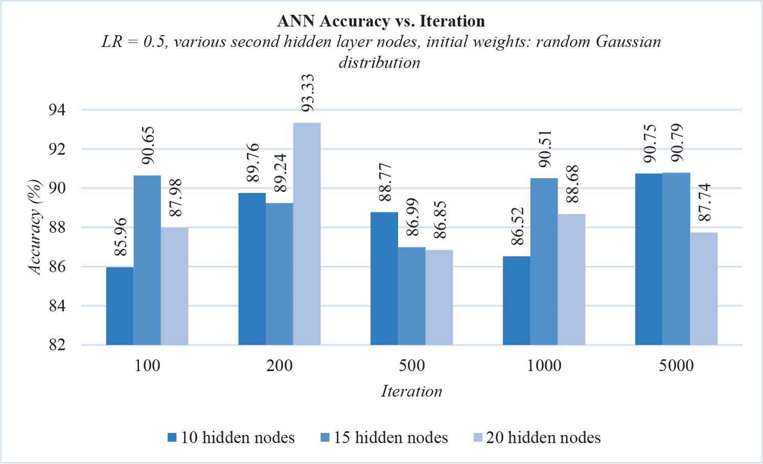
The accuracy of backpropagation gradient descent with various nodes in the second hidden layer.
4.1.3. Lowering error vs. iteration graph oscillation
Even though the accuracy was decent, the error vs. iteration graph showed extreme oscillation. To minimize the oscillation, we tried lowering the learning rate. The following experiments used the architecture with 2 hidden layers that reached the highest accuracy, that is, with 20 nodes in the second hidden layer. The results were as seen in Figure 6.
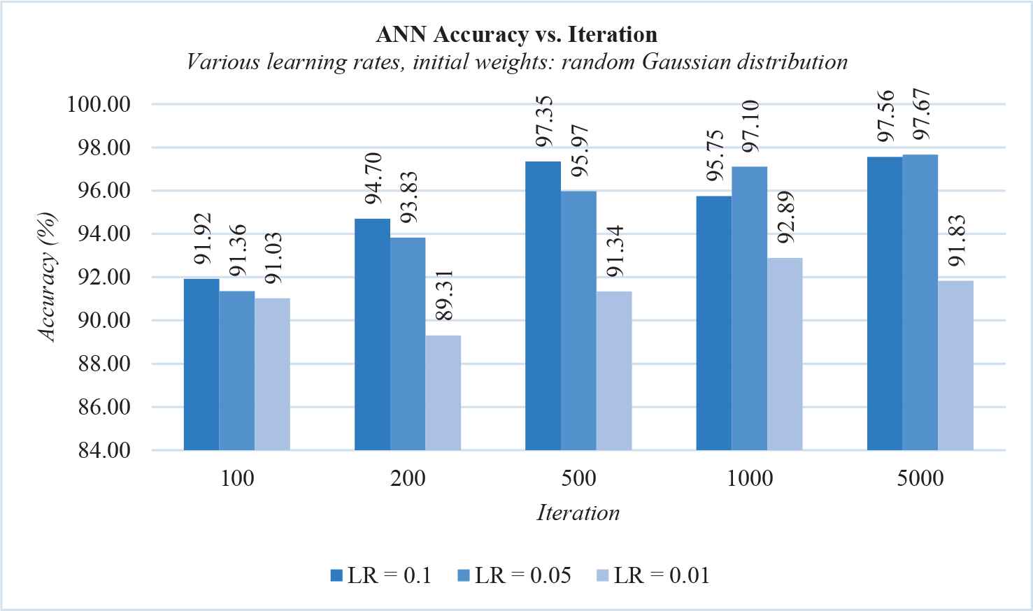
The average accuracy of backpropagation gradient descent with various learning rates.
The average accuracy shown in Figure 6 was obtained from doing 3 experiments for each configuration variations. The Error vs. Iteration graph of the experiments described in Figure 6 had much less oscillation than the experiments with the learning rate of 0.5, as can be seen in Figure 7.
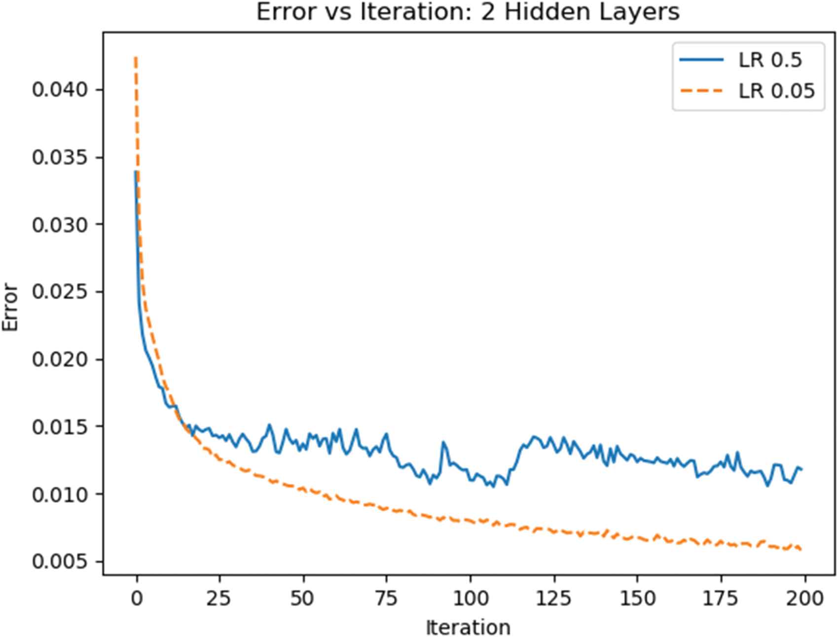
Error vs. iteration for 2 hidden layers (26 and 20 nodes each), LR 0.5 (solid), and LR 0.05 (dashed), trained over 200 iterations.
From the data in Figure 6, we can see that the best-performing ANN was the one with a learning rate of 0.05 and trained over 5000 iterations. The maximum accuracy for this configuration was 97.98%, with the error vs. iteration graph as seen in Figure 8. The confusion matrix is as seen in Table 1, with colored cells showing true positive predictions.
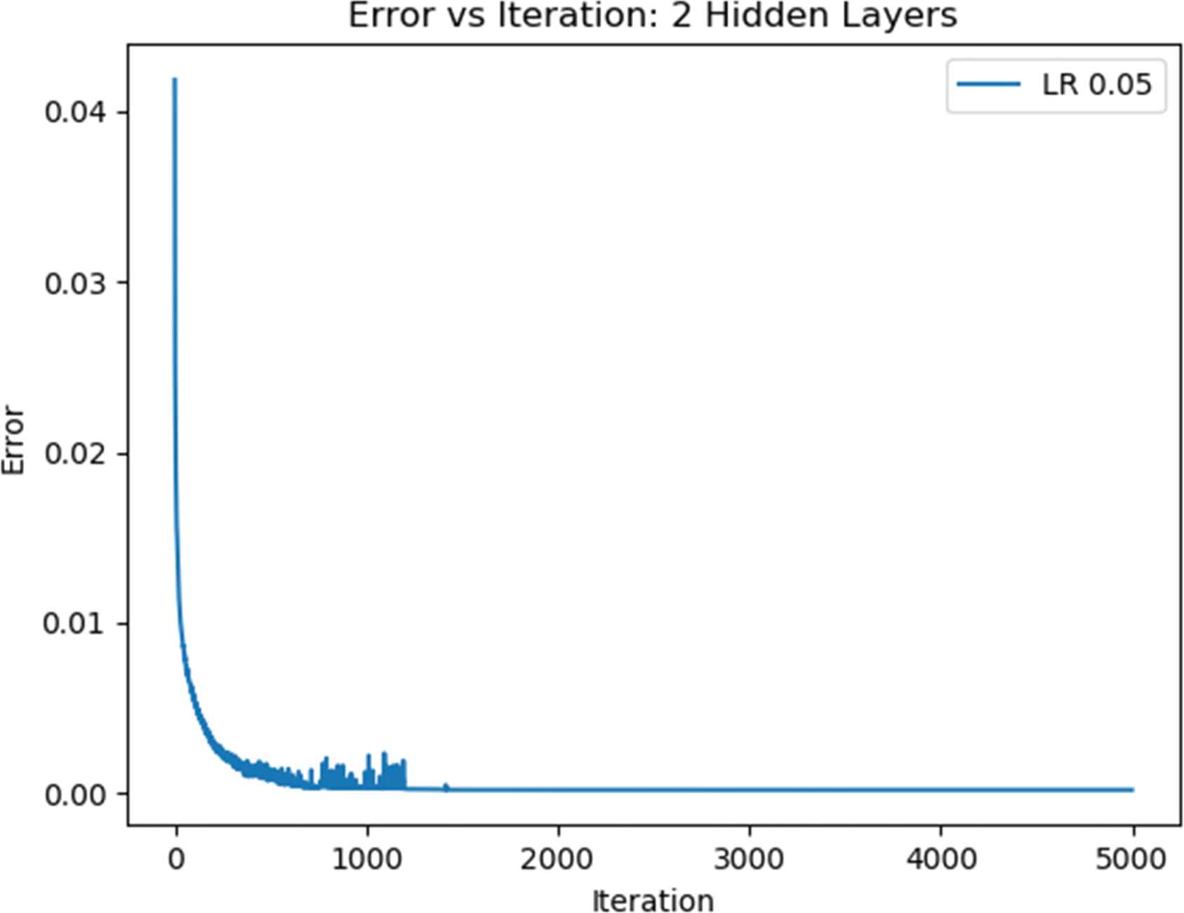
Error vs. iteration for 2 hidden layers (26 and 20 nodes each), LR 0.05, trained over 5000 iterations.
| Predicted Class | ||||||||
|---|---|---|---|---|---|---|---|---|
| 1 | 2 | 3 | 4 | 5 | 6 | 7 | ||
| Actual Class | 1 | 0 | 0 | 0 | 3 | 0 | 0 | 0 |
| 2 | 0 | 0 | 0 | 2 | 0 | 0 | 0 | |
| 3 | 0 | 0 | 0 | 0 | 0 | 0 | 0 | |
| 4 | 0 | 0 | 0 | 988 | 18 | 2 | 0 | |
| 5 | 0 | 0 | 0 | 13 | 368 | 1 | 0 | |
| 6 | 0 | 0 | 0 | 3 | 1 | 641 | 0 | |
| 7 | 0 | 0 | 0 | 0 | 0 | 0 | 89 | |
Confusion matrix of the maximum-accuracy configuration.
As can be seen above, the ANN classifies data with the ITEI score of 1 and 2 as 4. This is most likely caused by the very little amount of data labeled with ITEI score of less than 4 in the training data.
4.2. GIS Map Presentation
A GIS map presenting the average ITEI score of each district in Indonesia was also created to allow executives to evaluate the sample data easily. The dataset containing individual data had to be processed manually in Microsoft Excel using the PivotTable feature to convert the individual primary key to regional primary key before joining it with spatial data in the ArcGIS Pro software, so the data in the map are not real-time data. An example of individual data is shown in Picture 1, while the processed data of Picture 1 is shown in Picture 2. The joined data can be seen in the screenshot shown in Picture 3.
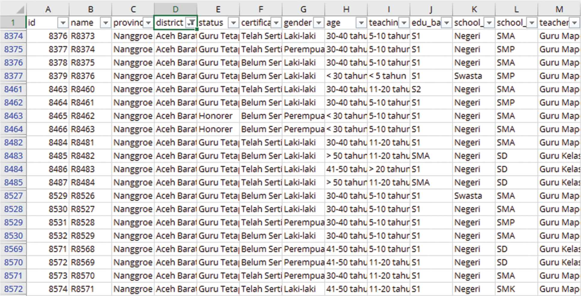
An example of the original dataset (individual data).

An example of the processed data (regional data).
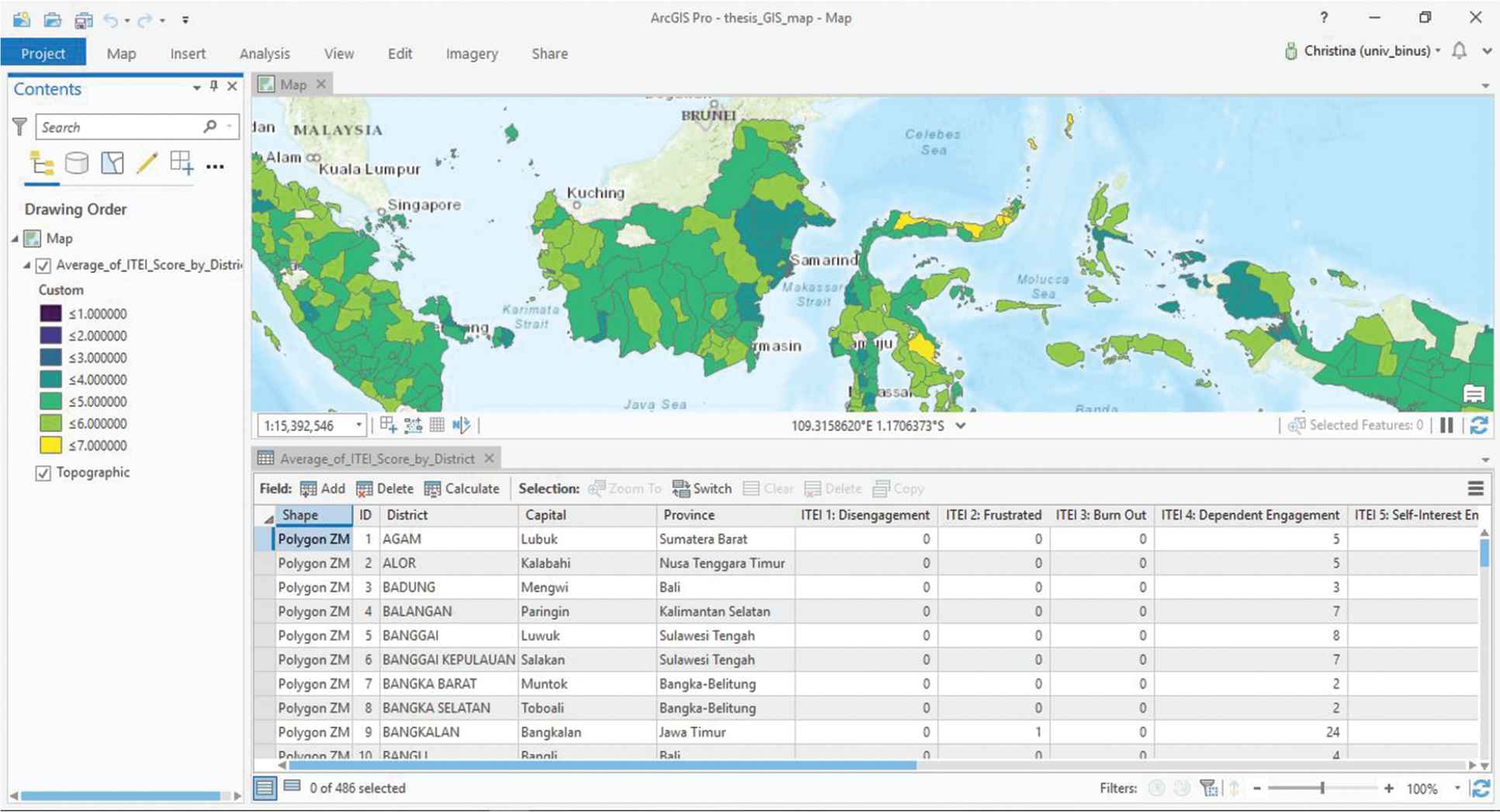
A screenshot of the data being processed in ArcGIS Pro.
The map was then published to the ArcGIS Online system and can be accessed as an embed map at http://www.itei.me/peta; the screenshot can be seen in Picture 4.

The embed GIS map as seen in http://www.itei.me/peta.
5. CONCLUSION
From the results, we can conclude that the optimal architecture of the ANN is 44 input nodes, 26 and 20 nodes in the first and second hidden layer respectively, and 7 output nodes. The optimal learning rate is 0.05, especially when trained over 5000 iterations. This configuration yielded an average accuracy of 97.67% and the maximum accuracy of 97.98%. The GIS map created to visualize the data was also able to present the data accurately, even though it must be updated manually every time a batch of new data comes in.
For future work, the ANN built in this research may be tested on more real data.
6. DECLARATIONS
List of abbreviations:
ANN: Artificial Neural Network
LR: Learning Rate
ITEI: Indonesian Teacher Engagement Index
CONFLICT OF INTEREST
Authors have no conflict of interest
ACKNOWLEDGMENT
We say thanks to Bina Nusantara University, the Indonesian Ministry of Research and Higher Education for supporting this research. We also want to say thanks to the Indonesian Ministry of Education and Culture and the Indonesian Directorate of Teachers and Educational Manpower for the help in collecting the national data.
REFERENCES
Cite this article
TY  - JOUR
AU  - Sasmoko Buddhtha
AU  - Christina Natasha
AU  - Edy Irwansyah
AU  - Widodo Budiharto
PY  - 2019
DA  - 2019/11/15
TI  - Building an Artificial Neural Network with Backpropagation Algorithm to Determine Teacher Engagement Based on the Indonesian Teacher Engagement Index and Presenting the Data in a Web-Based GIS
JO  - International Journal of Computational Intelligence Systems
SP  - 1575
EP  - 1584
VL  - 12
IS  - 2
SN  - 1875-6883
UR  - https://doi.org/10.2991/ijcis.d.191101.003
DO  - 10.2991/ijcis.d.191101.003
ID  - Buddhtha2019
ER  -