
2-Dimension Linguistic Bonferroni Mean Aggregation Operators and Their Application to Multiple Attribute Group Decision Making
- DOI
- 10.2991/ijcis.d.191125.001How to use a DOI?
- Keywords
- MAGDM; Bonferroni mean operator; 2-dimension linguistic weight Bonferroni mean aggregation operator; 2-dimension linguistic variable; 2-dimension linguistic lattice implication algebra
- Abstract
The aim of this paper is to provide a multiple attribute group decision making (MAGDM) method based on the 2-dimension linguistic weight Bonferroni mean aggregation (2DLWBMA) operator. Firstly, the new operations of 2-dimension linguistic variables are defined. Then, the 2-dimension linguistic Bonferroni mean aggregation operator is proposed to describe the correlations of input arguments. Subsequently, the 2DLWBMA operator is investigated to consider the importance of attributes. Furthermore, a novel MAGDM method is introduced and two illustrative examples are given.
- Copyright
- © 2019 The Authors. Published by Atlantis Press SARL.
- Open Access
- This is an open access article distributed under the CC BY-NC 4.0 license (http://creativecommons.org/licenses/by-nc/4.0/).
1. INTRODUCTION
Multiple attribute group decision making (MAGDM) methods refer to ranking the limited alternatives or selecting the best one according to the evaluation results provided by different decision makers. MAGDM methods have been widely applied in many areas, such as economic, society, science and management and so on. Among some MAGDM problems, the decision makers prefer to evaluate the alternatives on the qualitative attributes by linguistic variables (LVs) rather than crisp numbers. Since Zadeh [1–3] introduced the notion of LV, researchers have developed many kinds of methods to rank the alternatives according to the values of LVs [4–10]. However, in some real MAGDM problems, besides the linguistic evaluation values of the attributes, the decision maker still uses LVs to represent his or her self-assessment on the given evaluation results. For describing such phenomena, Zhu et al. [11] proposed the concept of 2-dimension linguistic variable (2DLV). A 2DLV includes two classes of LVs, where the
The main advantage of 2DLVs is that it can distinguish indetermination between decision making problems and subjective understanding. By use of 2DLVs, the decision makers can better express their opinions. Up to now, the research achievements of 2-dimension linguistic information can be classified into three categories: 2DLVs [12–17], 2-dimension uncertain linguistic variables (2DULVs) [18–28], and hesitant fuzzy 2-dimension linguistic variables (HF2DLVs) [29,30]. Since there exist two classes of LVs in a 2DLV, the operations of 2DLVs become more difficult and complex than those of LVs. For simplicity of calculation, many existing 2DLV operations only take the minimum values of the
Bonferroni mean (BM) operator, as a useful aggregation operator, has the ability to capture the interrelationships between input arguments. So far, BM operator has been widely extended to fuzzy linguistic environment [6,33–38], intuitionistic fuzzy linguistic environment [39–44], hesitant fuzzy environment [45] and pythagorean fuzzy circumstance [46] for handling the increasingly complex fuzzy systems and decision systems. Wei et al. [6] developed the uncertain linguistic BM operator and the uncertain linguistic geometric BM operator for aggregating uncertain linguistic information. Liu et al. [41] extended BM operator to the intuitionistic linguistic environment. Dutta et al. [34] applied the extended Bonferroni Mean (EBM) in linguistic 2-tuple environment to capture heterogeneous interrelationship among the attributes. Tian et al. [35,36] combined BM operator with simplified neutrosophic linguistic numbers and gray linguistic numbers to deal with the corresponding MADM problems. Combing the generalized partitioned Bonferroni mean (PBM) operator with linguistic neutrosophic numbers, Wang et al. [37] proposed the linguistic neutrosophic generalized weighted partitioned Bonferroni mean (LNGWPBM) aggregation operator to solve MAGDM problems. However, in some 2-dimension linguistic MAGDM problems, because the evaluation values of attributes are extended to two classes of LVs, the relationships between input arguments may be more complicated. In order to capture the interrelationships between input 2DLVs, it is necessary to extend BM operator into 2-dimension linguistic decision making environment.
Further, we list some extended BM methods in different application environments to convenient the readers by using the following tabular (see Table 1).
| Applications | Some Extended BM Methods |
|---|---|
| Fuzzy linguistic environment | Beliakov's method [33], Dutta's method [34], Tian's methods [35,36], Wang's method [37], Wei's method [6], Yager's method [38] |
| Intuitionistic fuzzy linguistic environment | Das's method [39], Heyd's method [40], Liu's methods [41,42], Zhang's method [43], Zhou's method [44] |
| Hesitant fuzzy linguistic environment | Zhu's method [45] |
| Pythagorean fuzzy linguistic environment | Nierx's method [46] |
| 2-dimension fuzzy linguistic environment | Liu's method [25], Yin's method [32], the proposed method |
BM = Bonferroni Mean.
Some extended BM methods in different application environments.
In 2-dimension linguistic MAGDM problems, Yin et al. [32] have combined trapezoidal fuzzy 2-dimensional linguistic information with a PBM operator to address the 2-dimension linguistic decision making problems. Liu et al. [25] have proposed the 2-dimensional uncertain linguistic weighted Bonferroni mean (2DULWBM) operator and the 2-dimensional uncertain linguistic improved weighted Bonferroni Harmonic mean (2DULIWBHM) operator. However, this paper combine 2DLVs with BM operators for different aspects. Concretely, the operations of 2DLVs are improved as stated in the above, where the
Motivated by the above ideas, we intend to
Define some new operations of 2DLVs.
Establish the 2-dimensional linguistic Boneferroni mean aggregation (2DLBMA) operator and the 2DLWBMA operator.
Investigate the properties and special cases of the 2DLBMA operator.
Propose a novel decision making method based on the 2DLWBMA operator.
Demonstrate the feasibility and practicality of the proposed method.
The remainder of this paper is established as follows: Section 2 reviews 2DLV and BM operator. In Section 3, some new operations of 2DLVs are developed and their properties are discussed. In Section 4, the 2DLBMA operator and the 2DLWBMA operator are proposed for 2DLVs. Section 5 provides a novel decision making approach based on the 2DLWBMA operator. In Section 6, two illustrative examples are given. Section 7 concludes this paper.
2. PRELIMINARIES
This section reviews some basic notions of 2DLV and BM operator.
2.1. 2DLV
Definition 1.
[11] Let
For describing the complicated relationships between 2DLVs, Zhu et al. [47] proposed the concept of a 2-dimension linguistic lattice implication algebra (2DL-LIA). The method for comparing two 2DLVs is provided in a 2DL-LIA as follows.
Definition 2.
[47] Let
If
If
If
If
Usually, the parameter
2.2. BM Operator
Since BM operator can capture the interrelationship between input arguments, it has been widely applied in MAGDM problems.
Definition 3.
[48] Let
BM operator satisfies the following properties:
If
If
If
Especially,
3. NEW OPERATIONS OF 2DLVs
According to the Definition 1, in a 2DLV
Definition 4.
Let
Remark.
In Definition 4, there exist the mutual transformations between the
Example 1.
Let
By Definition 4, we can compute that
In the following, some propositions of the new operational rules are discussed.
Proposition 1.
Let
Proof.
The proof of (1) can be obtained according to Definition 4.
Firstly, we give the proof of (2). On one hand,
On the other hand,
Hence we have
Then, the proof of (4) is given as follows. Since
On the other hand,
Hence
Similarly, (3) and (5)–(8) can be proved, which are omitted here.
Proposition 2.
Let
Proof.
Suppose
(1) Because
And we have
Since
then according to Definition 2,
(2) Because
Since
(3) Suppose
Then we have
Since
It follows that
Therefore
that is
And
Since
Similarly, (4) can be proved, which is omitted here.
(5) We can prove
When
Assume
Then, when
Because
then by (3), we have
that is
Now, we have
(6) can be proved similarly by the mathematical induction.
Proposition 3.
Let
Proof.
(1) We can prove
by the mathematical induction on
When
Assume
Then, when
Now, we have
Similarly, (2)–(6) can be proved by the mathematical induction, which are omitted.
4. 2DLBMA OPERATOR AND 2DLWBMA OPERATOR
In this section, based on BM operator and the new operational rules of 2DLVs, we develop the 2DLBMA operator to deal with MAGDM problems.
4.1. 2DLBMA Operator
Definition 5.
Let
is called the 2DLBMA operator.
The 2DLBMA operator is a useful tool to capture the interrelationship between the attributes in 2-dimension linguistic MAGDM environment.
Example 2.
Let
According to Definition 5, we can compute that
The following theorem shows that the aggregation value of 2DLVs, which is aggregated by the
Theorem 4.
Let
Proof.
The proof of Theorem 4 includes three steps, which are given in the following.
Step 1 By Definition 4,
then by Proposition 3, we have
It follows that
Step 2 By Definition 4, we can obtain that
Step 3 Based on Step 2 and Definition 4, we have
Next, we can prove that the
Theorem 5.
(Idempotency) Let
Proof.
Because
Theorem 6.
(Monotonicity) Let
Proof.
Because
Theorem 7.
(Commutativity) Let
Proof.
According to Proposition 1 (4), the conclusion can be obtained.
Theorem 8.
(Boundedness) Let
Proof.
Since for all
Subsequently, some special cases of the
Case 1 If
which is called the 2-dimension linguistic generalized mean aggregation operator.
Case 2 If
which is called the 2-dimension linguistic mean aggregation (2DLMA) operator.
Case 3 If
which is called the 2-dimension linguistic geometric mean aggregation (2DLGMA) operator.
4.2. 2DLWBMA Operator
In real MAGDM environment, the weights of attributes are usually different, hence the
Definition 6.
Let
is called the 2-dimension linguistic weight Bonferroni mean aggregation (2DLWBMA) operator, where
Obviously, if the weight vector
Example 3.
Let
According to Definition 6, we can compute that
The following theorem shows that the aggregated result of 2DLVs by the
Theorem 9.
Let
Proof.
This proof includes three steps.
Step 1 By Definition 4,
Then by Proposition 3 (1), we have
Further, according to Proposition 3 (1), we have
Step 2 By Definition 4, we can obtain that
Step 3 Based on Step 2 and Definition 4, we have
5. A MAGDM METHOD BASED ON THE 2DLWBMA OPERATOR
In a MAGDM problem, let
The expert
The proposed method involves the following steps:
Step 1 Normalize the 2DLV decision matrix.
Since the set of attributes
Step 2 Calculate the collective decision information by the
Based on the normalized 2DLV decision matrixes
where
Step 3 Calculate the overall evaluation value of each alternative base on the
Based on the aggregated 2DLV decision matrix
where
Step 4 Compare the obtained overall evaluation values
Step 5 Rank all the alternatives or select the best one(s) in accordance with the ranking of
Step 6 Ends.
6. EXAMPLES ILLUSTRATIONS
In this section, we use the proposed MAGDM method based on the
6.1. Application to the Technological Innovation Ability Evaluation Problem
For the technological innovation ability evaluation problem cited from literature [23], the proposed MAGDM method based on the
Example 4.
[23] A practical use of the proposed approach involves the technological innovation ability evaluation of the four enterprises
Let
The 2DLV decision matrixes
6.1.1. Illustration of the proposed method
The proposed method based on the
Step 1 Normalize the 2DLV decision matrixes.
Since all the attributes are the benefit attributes, the evaluation values of 2DLVs do not need normalizing.
Step 2 Aggregate the evaluation values of each expert by the
Based on the 2DLV decision matrixes
Step 3 Calculate the overall evaluation value of each alternative.
Based on the 2DLV aggregated decision matrix
Here let
Step 4 Rank
According to Definition 2, we can obtain the ranking order of
Step 5 Rank all the alternatives in accordance with the ranking of
Thus the ranking order of the alternatives is
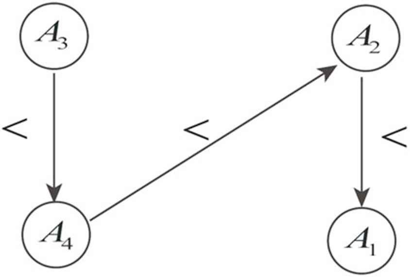
The ranking order of alternatives.
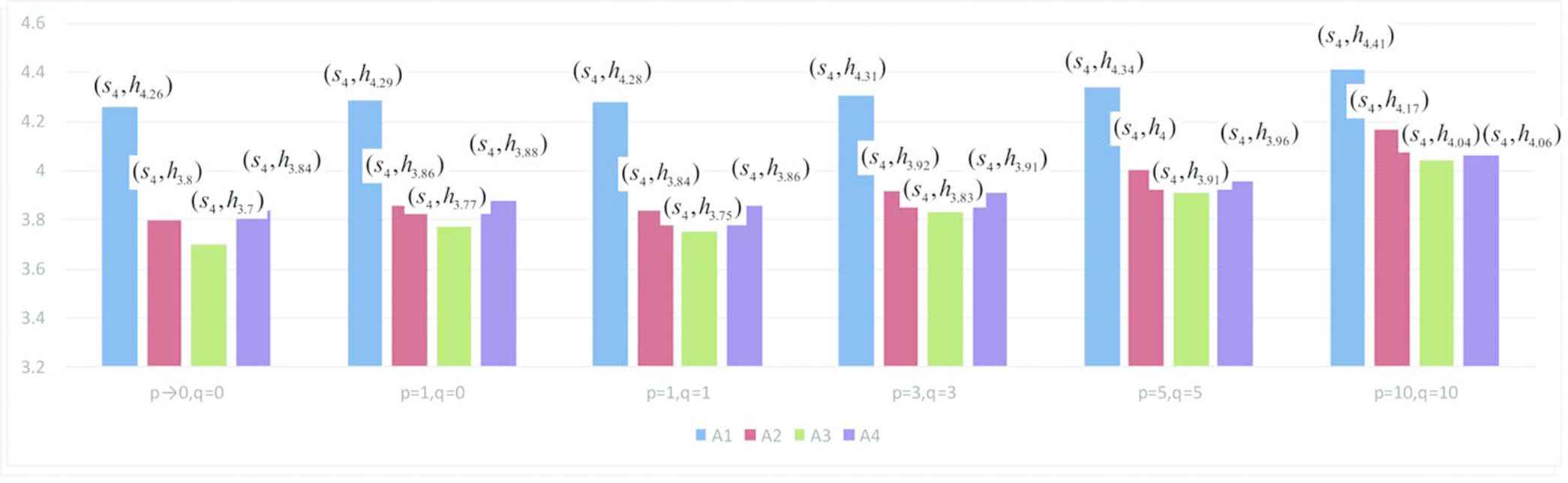
6.1.2. Exploration of the parameters' influence
Here in this example, for illustrating the influences of the parameters
| The Values of p and q | The Evaluation Values ri of Alternatives | Ranking Results |
|---|---|---|
Ranking orders of the alternatives under different values of
Ranking orders of the alternatives under different values of p and q.
From Table 2, we can see that the best alternative is always
When
When
When
According to the outcomes of Table 2, it shows that the
6.1.3. Sensitivity analysis of the weight vector
Sensitivity analysis of the weight vector, as an important part of MAGDM, has been developed to assess the stability of the ranking [16,50,51].
When we conduct the weight sensitivity analysis, only one criterion is focused at a time. That is, if a criterion changes, the other criteria are assumed to be changed uniformly in order to remain normalized.
Memariani et al. [51] provided a new method for the weight sensitivity analysis in MADM. Let
By use of Memariani's method [51], we only conduct the weight sensitivity analysis of attributes in Example 4. In addition, we only analyse the
| Attribute | Original Weights | Stability Intervals of Weight |
|
|---|---|---|---|
| Min | Max | ||
| 0.25 | 0.23 | 0.26 | |
| 0.27 | 0.27 | 0.29 | |
| 0.25 | 0.19 | 0.28 | |
| 0.23 | 0 | 0.23 | |
Sensitivity analysis for the weight vector of attributes.
In Table 3, it indicates that the ranking order solved by the proposed method is resistant to change in Example 4 for the different stability intervals of weights. The weight stability interval of the attribute
6.1.4. Comparison analysis
In this subsection, different decision making approaches are applied to solve Example 4. These decision making approaches include respectively the decision making approach based on the generalized triangle fuzzy number (TFN) [15], the decision making approach based on the extended Interactive and Multiple Attribute Decision Making (TODIM) method [23], the decision making approach based on the power operator [20] and the decision making approach based on the 2DLV with two 2-tuples [17].
Since the decision making approach based on the generalized TFN [15] can only handle MADM problems in 2-dimension linguistic environment, it may as well select the second decision maker's decision matrix
Moreover, the decision making approach based on the extended TODIM method [23] mainly considers 2DULVs. Since a 2DLV is the special case of the corresponding 2DULV, we can replace 2DULVs with 2DLVs in this 2-dimension linguistic computational model.
Similarly, the decision making approach based on the power operator [20] considers 2DULVs. we also replace 2DULVs with 2DLVs in this 2-dimension linguistic computational model.
Then we use the decision making approach based on the 2DLV with two 2-tuples [17] to solve Example 4, it should transform the 2DLV decision matrix into the 2DLV decision matrix with two 2-tuples.
The ranking results by different approaches are shown in Table 4.
| Methods | Ranking Results |
|---|---|
| Yu's method [15] (based on | |
| the 2DLWA operator) | |
| Zhu's method [17] (based | |
| on the 2DLWAA operator) | |
| The proposed method | |
| with |
|
| Liu's method [23] (based on | |
| the extended TODIM method) | |
| Liu's method [20] (based on | |
| the power operator) | |
| The proposed method with |
2DLWA = 2-dimension linguistic weighted averaging; 2DLWAA = 2-dimension linguistic weighted arithmetic aggregation.
Ranking results by different methods.
From Table 4, the best alternative is
Because Yu's method [15], Zhu's method [17] and the proposed method with
Liu's method [20] based on the power operator considers the correlations of attributes. Moreover, Liu's method [23] based on the extended TODIM method considers the bounded rationality of decision makers. Furthermore, the proposed method can not only capture the correlations of attributes, but also describe the rationality of decision makers. Therefore, the results solved by Liu's method [20], Liu's method [23] and the proposed method with
In a word, the proposed method with 2DLVs for MAGDM problems has the following advantages. Firstly, the new operations of 2DLVs may be more reasonable than the existing operations. This new operations, that is, the
In fact, the decision makers can select suitable parameter values in the proposed method according to the actual decision situations and their experience or knowledge. In other words, taking different parameter values of
6.2. Application to the Landfill Site Selection Problem
By use of the proposed MAGDM method, we can solve the landfill site selection problem which is cited from literature [49]. It concludes that the proposed method can not only handle MAGDM problems within 2-dimension linguistic environment, but also deal with MAGDM problems within fuzzy linguistic environment.
Example 5.
[49] The practical example involves a landfill siting problem in KS City. Considering the dense population of KS City, there are four candidate locations
The LTS
6.2.1. Illustration of the proposed method
Example 5 is solved by the proposed method based on the
Step 1 Normalize the 2DLV decision matrix.
In order to apply the proposed MAGDM method to rank the four candidate locations, we assume that the decision maker selects the same linguistic term
Since the attributes
The original 2DL decision matrix
Step 2 Calculate the overall evaluation value of each alternative.
Based on the normalized 2DLV decision matrix
Here let
Step 3 Rank
According to Definition 2, we can obtain the ranking order of
Step 4 Rank all the alternatives and select the best one(s) in accordance with the ranking of
Thus the ranking order of the alternatives is
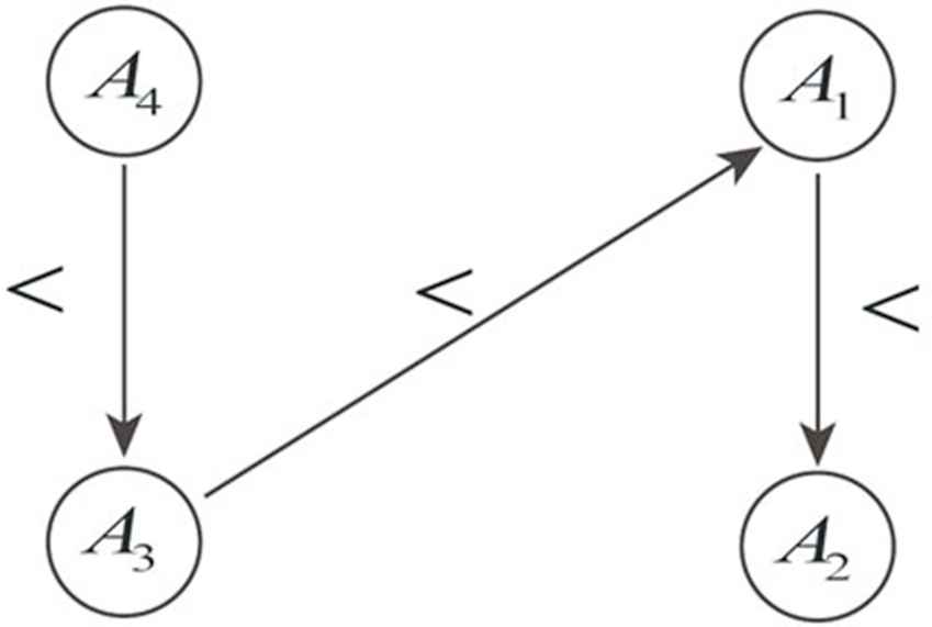
The ranking order of alternatives.
6.2.2. Exploration of the parameters influence
For illustrating the influences of the parameters
| The Values of p and q | The Evaluation Values ri of Alternatives | Ranking Results |
|---|---|---|
Ranking orders of the four candidate locations under different values of
From Table 5, we can see that the relationships among alternatives
When the
When the
When
According to the outcomes of Table 5, it shows that the
6.2.3. Sensitivity analysis of the weight vector
In order to illustrate the influences of linguistic weight vector on the ranking results, a sensitivity analysis is conducted in Example 5.
In Subsection 6.2.3, we have discussed Memariani's method [51]. Applying Memariani's method, we can also normalize the linguistic weight vector of attributes.
We only discuss the
| Attribute | The Original Linguistic Weight | Stability Intervals of Weight |
|
|---|---|---|---|
| Min | Max | ||
| H ( |
L ( |
AH ( |
|
| MH ( |
ML ( |
AH ( |
|
| H ( |
M ( |
AH ( |
|
| MH ( |
ML ( |
AH ( |
|
| MH ( |
ML ( |
AH ( |
|
| M ( |
VL ( |
VH ( |
|
| ML ( |
AL ( |
AH ( |
|
Sensitivity analysis for the weight vector of attributes.
From Table 6, we find that the ranking order solved by the proposed method is fully resistant to change in the importance of the attribute
7. CONCLUSIONS
Since a 2DLV adds a class of LV to express the decision maker's self-assessment, it can better express fuzzy information. In order to embody the innate character of the decision maker's self-assessment, this paper defined the new operations of 2DLVs. In the new operations of 2DLVs, the operations of the
In future, based on this new operational rules of 2DLVs, other kinds of aggregation operators should be proposed to deal with the corresponding situations in real 2-dimension linguistic decision making. Moreover, the proposed 2DLWBMA operator should be considered to extend into other fuzzy environments for solving MAGDM problems.
CONFLICT OF INTEREST
We declare that we do not have any commercial or associative interest that represents a conflict of interest in connection with the work submitted.
AUTHORS' CONTRIBUTIONS
Jianbin Zhao did the formal analysis, editing, and Software. Hua Zhu was involved with the resources and writing original draft. Both the authors were involved with the conceptualization, methodology, validation, investigation and writing-review.
ACKNOWLEDGMENTS
This work is partially supported by the Natural Science Foundation of China (Grant No. 61673320 and 61772476). The authors also gratefully acknowledge the helpful comments and suggestions of the reviewers.
REFERENCES
Cite this article
TY  - JOUR
AU  - Jianbin Zhao
AU  - Hua Zhu
PY  - 2019
DA  - 2019/12/06
TI  - 2-Dimension Linguistic Bonferroni Mean Aggregation Operators and Their Application to Multiple Attribute Group Decision Making
JO  - International Journal of Computational Intelligence Systems
SP  - 1557
EP  - 1574
VL  - 12
IS  - 2
SN  - 1875-6883
UR  - https://doi.org/10.2991/ijcis.d.191125.001
DO  - 10.2991/ijcis.d.191125.001
ID  - Zhao2019
ER  -