
Exploitation of Social Network Data for Forecasting Garment Sales
- DOI
- 10.2991/ijcis.d.191109.001How to use a DOI?
- Keywords
- Social Media Data; Forecasting; Naïve Bayes; Sentiment analysis; Fuzzy forecasting model
- Abstract
Growing use of social media such as Twitter, Instagram, Facebook, etc., by consumers leads to the vast repository of consumer generated data. Collecting and exploiting these data has been a great challenge for clothing industry. This paper aims to study the impact of Twitter on garment sales. In this direction, we have collected tweets and sales data for one of the popular apparel brands for 6 months from April 2018 – September 2018. Lexicon Approach was used to classify Tweets by sentence using Naïve Bayes model applying enhanced version of Lexicon dictionary. Sentiments were extracted from consumer tweets, which was used to map the uncertainty in forecasting model. The results from this study indicate that there is a correlation between the apparel sales and consumer tweets for an apparel brand. “Social Media Based Forecasting (SMBF)” is designed which is a fuzzy time series forecasting model to forecast sales using historical sales data and social media data. SMBF was evaluated and its performance was compared with Exponential Forecasting (EF) model. SMBF model outperforms the EF model. The result from this study demonstrated that social media data helps to improve the forecasting of garment sales and this model could be easily integrated to any time series forecasting model.
- Copyright
- © 2019 The Authors. Published by Atlantis Press SARL.
- Open Access
- This is an open access article distributed under the CC BY-NC 4.0 license (http://creativecommons.org/licenses/by-nc/4.0/).
1. INTRODUCTION
Due to the advent of social media, people, in general, have, like never before, been able to express and share their opinions about their various shopping experiences. In a consumer and market research framework, knowing about consumer experiences is crucial for the companies to improve their products and services they provide. Companies are now in a fierce competition to collect information about the experiences and opinions of their customers from social media as this information provides them with the valuable insights, which can be used to improve the satisfaction of their customers. Traditionally, companies relied on sales forecasting models to estimate their future product sales, which in turn help them in the strategic and effective management of their business operations. However, embedding consumer opinions into sales forecast models and studying their influence on the sales is increasingly becoming a new research trend [1]. There is a shift from the study of effects of marketing and advertisement on product sales to the study of social media influence. Social media is considered to be the digital word-of-mouth platform, which significantly influences consumers shopping behavior and thus, the product sales [2]. Many studies have explored the relationship between consumer sentiments on social media and the product sales [3]. Fashion industry is grappling with numerous challenges of understanding their customers’ opinions and adjusting their business models accordingly [4]. The recent trend of fast fashion is evident to the fact that consumers are rapidly evolving in terms of their changing preferences for new products, designs and features, and also the short product life cycle. Many industries such as television, telecommunication, banks, etc., tap social media to extract customer opinions, and adjust their operations based on the insights derived from social media [5]. However, there is a dearth of research on models in the fashion industry that study the factors such as social media and its effects on product sales. Fashion industry faces operational challenges emanating from the uncertainty in product demand and consumer choices. In this context, traditional forecast models that take into account the effects of marketing campaigns and advertisements on product sales fail to capture the effects of social media. Given the need for real time sales forecast in order to be able to manage various logistics related problems such as inventory, fashion industry needs to consider studying the effects of social media on the sales.
Motivated by the aforementioned problem facing garment industry, this research, aims to forecast garment sales by exploiting twitter data and investigating its influence of twitter as a social media on garment sales. Focusing into line, this study presents a hybrid sales forecast model “Social Media Based Forecasting (SMBF)” which is a fuzzy time series forecasting model that maps historical information of the sales and the “Impact of sentiments from social media”(Fuzzy Sentiment Impact on Sales [FSIS] model) on garment sales. This research uses real twitter data and historical sales data for an Italian fashion brand, and applied developed model to examine its forecast performance. We believe that this paper is the first endeavor to use sales forecast model on social media data in a fashion industry. In this study, we propose a sales forecast model that is combined with sentiment analysis of social media platform, and we investigate if the performance of garment sales forecast can be improved using this model. The results from this study contributes to addressing overarching research question of forecasting fashion product sales by exploiting social media data, and it can provide decision makers in fashion industry with significant practical insights to optimize their business strategies. Moreover, we show that given the high performance of the model presented in this paper, it is possible to enable sustainable garment production as it would prevent the risk of over production of garments.
Detailed discussion of the existing literature is explained in Section 2. Experimental design and methodology is discussed in Section 3. This is followed by experimental results in Section 4, illustrating the classification results, correlation results and the model performance. Sections 5 and 6 explain the results, discussion and conclusion.
2. LITERATURE REVIEW
This section discusses existing literature related to sales forecasting in a fashion industry, in general, and the use of social media data based sales forecasting for various products. Maria E. Nenni, in paper [6], presents an excellent review of different existing sales forecasting methods used in fashion industry, and explores their suitability to forecast demands and sales with different characteristics. It is highlighted that inaccuracy or low performance of forecast models could be the result of unavailability of historical data, short selling and high level of uncertainty related to consumer preferences and satistication. Limitations of traditional sales forecast models such as auto-regressive (AR) model, extreme learning machine (ELM) model and artificial neural network (ANN) model are highlighted in the work [7] by studying the performance of newly developed ELM model with adaptive metrics of input and comparing its accuracy with the traditional ones. In the study carried out by [8], more accurate models based on fuzzy logic, data mining and neural network are used to improve the precision of sales forecasting in a clothing industry. The first study of consumer opinions in terms of online ratings given by consumers is studied [9], wherein Bass model is developed to forecast movie sales on box office. This study was the first approach to investigate the relationship between online reviews as a proxy for spread of consumers’ word-of-mouth and its influence on sales forecast. In a study done by [10], a linear regression model is used in combination with sentiment classifier to forecast box office sales, and the study (concluded) concludes that sentiments from Twitter (highly influence) have high influence on movie sales on box office. To forecast fluctuations in Amazon’s daily products sales, natural language processing is used in [11] to extract sentiments from online product reviews, and the relationship between sentiments and the product sales (have) has been studied. In a similar study done by [12], AR sentiment aware model has been applied to forecast revenue on box office by extracting sentiments from online blogs and their influence on sales was found significant. Another domain, such as earthquake forecasting, where twitter data is used to predict damages caused by earthquakes is studied in [13]. In this study, machine learning models such as naïve Bayes (NB) and support vector machine (SVM) are used to classify tweets related to earthquake incidents and further embedded with spatial smoothing and regression models to estimate the loss due to earthquake. Very interesting application of social media analytics is presented in the study by [14], where authors used deep learning methods to forecast disease outbreak from twitter data with high accuracy. Popularity prediction model based on deep learning is developed in [15], where they extracted social media data to predict overall public interest and social trend. Another interesting industry example of social media based prediction is presented in [16], where machine learning models are applied to derive sentiments from news and social media and used to predict stock prices. Study done by [17] presents a graph theory based convolutional neural network model to forecast propaganda in a political system and also to predict election outcomes in South Africa and Kenya by extracting sentiments from tweets. Due to the growing trend of fast fashion, product life cycle is shrinking rapidly, and therefore, traditional long-term sales forecast models are irrelevant and are not very useful. Short-term demand and replenishment forecasting in a fashion industry using deep learning methods based on real historical industry data is conducted in [18]. Moreover, the influence of consumer sentiments, derived from a big data stream of online customer reviews generated in an e-commerce industry, has been studied in [19] by applying efficient methods to visualize short term demand forecast. This study has emphasized that online consumer sentiments are the promising factor to forecast short-term demand at a product level. Consumer sentiments derived from social media platform such as twitter, are studied in [20] to gauge the current fashion market trend and to predict the consumer perception toward brands. Study in [21] provides a comprehensive discussion on the usefulness of social media data for the operational activities of the industries. It is observed that social media has proved to be a significant factor for understanding of (various social outcomes) consumer behavior and it has a high influence on today’s competitive digital market. In this respect, we aim to study the consumer sentiments from their tweets about fashion brand and to explore their influence on garment sales, which is the first study of its kind in a fashion industry domain.
3. EXPERIMENTAL DESIGN AND METHODS
This section presents the schema of all the steps involved in the SMBF model implementation. It is divided into sub-sections briefing different stages involved in the development of model.
Subsequently, research framework (adopted in) this study is explained in Section 3.1. In the following sections, the topics covered are as follows: data collection steps in Section 3.2, data preprocessing in Section 3.3, sentiment extraction from fashion brand tweets in Section 3.4, Exponential Forecast model explanation in Section 3.5, modeling uncertainty of tweet sentiments using fuzzy inference in Section 3.6, stepwise implementation of SMBF model in Section 3.7, and finally, forecasting performance measuring indicator is explained in Section 3.8.
3.1. Research Framework
Research outline is shown in Figure 1, which includes sales prediction exploiting social media data and sales data in the following steps:
Data Collection—To accomplish the task, Twitter and sales data spanning six months were collected from Italian fashion brand.
Data Preprocessing and Sentiment extraction—In this step, text mining technique is used for cleaning tweets. These cleaned tweets were then used for sentiment extraction using an enhanced NRC lexicon data and NB classifier. Classification results into three sentiment indicators Positive (Sp), Negative (Sn) and Neutral (Sne).
Examine correlation—Extracted sentiments from earlier stage were aggregated weekly and the relationship between the sentiments of the current week and sales of the upcoming week was examined. This step was carried out to investigate relationship between tweets and sales.
SMBF Model—After exploring the relationship between tweet sentiments and sales, this model is designed to forecast garment sales based on historical sales and sentiments from social media. To attain this, FSIS model was built to identify the uncertainty of sentiments in terms of corrective coefficient (Vs), which represents the sales variation factor with actual sales and this is implemented on Exponential Forecast (EF) to predict the final forecast from SMBF model.
Performance Validation—The model performance was validated using forecasting measure, Mean Absolute Performance Error (MAPE).
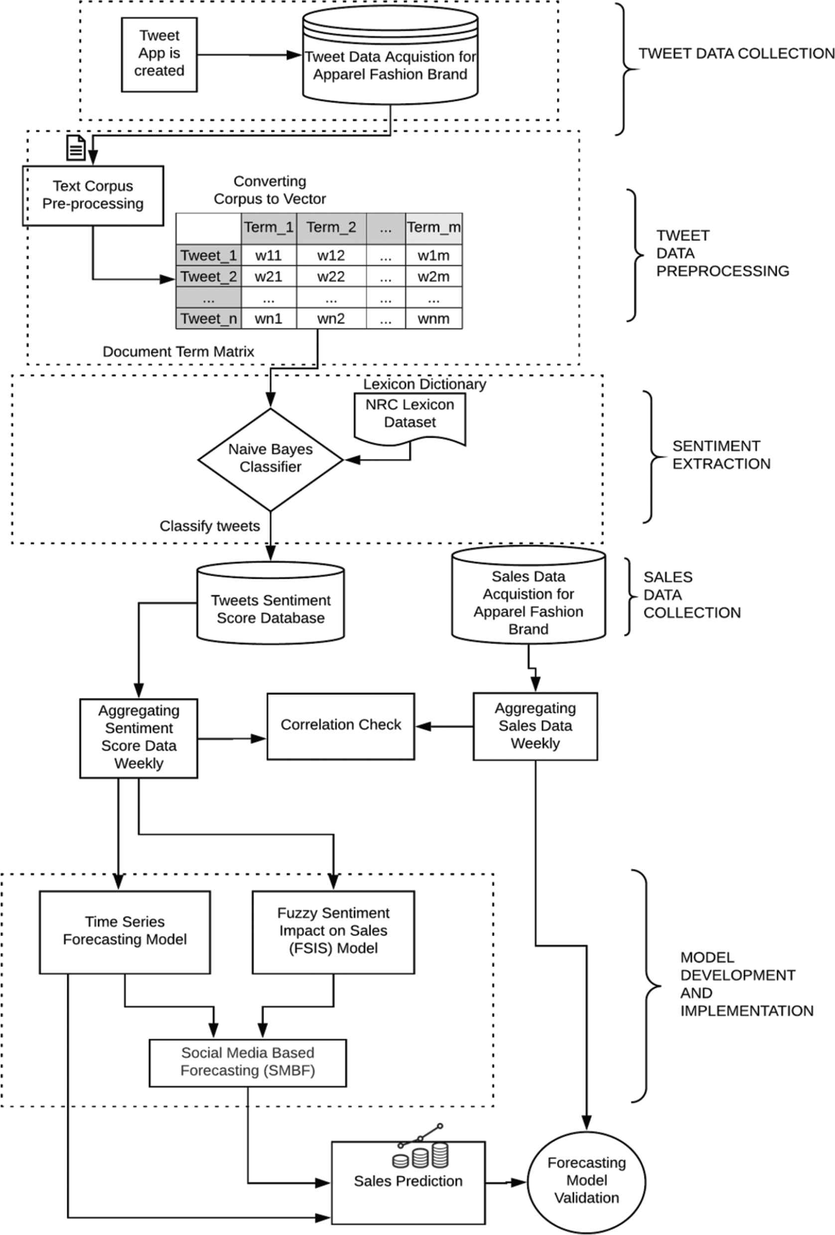
Research framework.
3.2. Data Collection
Data used in this work was collected for one of the Fashion apparel brands, spanning time period of six months from April 2018 and September 2018. This study uses two data forms, first, Twitter data, which were collected using tweet API by creating tweet app to get authentication key [22]. Open source tool “Rstudio” and its package “TwitterR” were used to request API to Twitter using Oauth access [20]. Semantic keywords with hashtag “Brand name” were applied on tweet retrieval string. Collected tweets attributes is shown in the Table 1 and total number of tweets collected for six months interval was 838 as shown in Table 2.
| Serial No. | Attribute | Type | Description |
|---|---|---|---|
| 1 | Text | String | This is the text of the Tweet. |
| 2 | Favorited | Boolean | Specifies if the Tweet has been liked by the authenticated user |
| 3 | Favorite_count | Integer | Specifies the count of the Tweet that has been liked by the users |
| 4 | ReplyToSN | String | If the represented Tweet is a reply, this field will contain the screen name of the original Tweet’s author |
| 5 | Created | String | This field states creation of Tweet at UTC time |
| 6 | Truncated | Boolean | If the original tweet exceeds the limit of 140 characters, the attribute “text” will be truncated and it will represented by ellipsis “…”. |
| 7 | ReplyToSID | String | If the specified Tweet is a reply, this field will contain the string representation of the original Tweet’s ID. |
| 8 | Id | Integer | It represents an unique identifier of a tweet |
| 9 | ReplyToUID | Integer | If the tweet is a reply, this attribute will give the integer representation of the original Tweet's author ID. |
| 10 | StatusSource | String | It represents source of the Tweet created via Web, Android, iphone, etc. |
| 11 | ScreenName | String | This field gives the “screen name” of the user |
| 12 | RetweetCount | Integer | Number of times particular Tweet has been retweeted |
| 13 | Place | Places | User's location |
| 14 | Retweeted | Boolean | It indicates if the Tweet has been retweeted |
| 15 | Longitude/latitude | Coordinates | Indicates user's geographical location |
Attributes of Tweet data.
| Month | Collected Tweets |
|---|---|
| April | 142 |
| May | 166 |
| June | 97 |
| July | 152 |
| Aug | 143 |
| Sep | 138 |
| Total | 838 |
Collected Tweets.
In the next step, sales data for the same interval of time as the Twitter data was collected, which accounts for the daily sales of garments.
3.3. Twitter Data Preprocessing
Twitter data collected in previous step was in an unstructured form as it contained many duplicates, urls, punctuation, etc. It was necessary to clean and normalize tweet for analysis. As the first step of preprocessing, manual screening of tweets were performed to confirm whether or not it belongs to the fashion apparel brand that we targeted. While exploring the tweets, synonyms of selected brand name were found in some tweets. Moreover, some of the tweets were also related to politics, games and some other issues, and therefore such tweets were removed. Secondly, as only text is required for sentiment analysis, first attribute shown in the Table 1 was chosen. Text mining was applied to remove duplicates, whitespaces, hashtags, urls, stop words, retweet entities and numbers [20]. As a result, the total count of tweets reduced to 313, which is 37.35 % of the actual collected data.
3.4. Algorithm Formalization for Sentiment Extraction (Or Mining?) from Tweets
This section discusses the methodology applied for the classification of tweets. Lexical approach was used to extract sentiments from tweets [23]. NRC lexicon dictionary [24] was used, which contains 5636 words labeled with “Positive” and “Negative.” For the tweet classification task, a probabilistic classifier “NB” algorithm [25] was used as it is the effective classification model for text classification. Moreover, it is highly scalable and it allocates the class labels of a finite set to feature vectors [23]. The algorithmic representation of NB is shown in Eq. (1).
For the mathematical formulation of this research task Twitter dataset T is considered, which is a set of tweets t and can be represented as
| Words |
Sentiment Class |
|---|---|
| Good | Positive |
| Sad | Negative |
| Honest | Positive |
Example of the lexicon dictionary dataset.
For each given tweet t in Twitter dataset T, NB computes posterior probability of classes of sentiments,
Further, from Eq. (2), denominator is dropped as P(t) will remain same for all sentiment class and it will have an impact on “argmax” [26]. Therefore, it can be transformed as shown in Eq. (3).
Therefore, Eq. (3) can be rewritten as below
This model follows the assumptions: position of the features (words) are not taken into account and the feature probabilities
Furthermore, formalization of the above equations was implemented for the ease of applying it in programming language illustrated in the Figure 2. It is assumed that the algorithm will calculate the maximum posterior probability for the occurrence of a word in a given tweet that is present in a lexical dataset. Therefore,
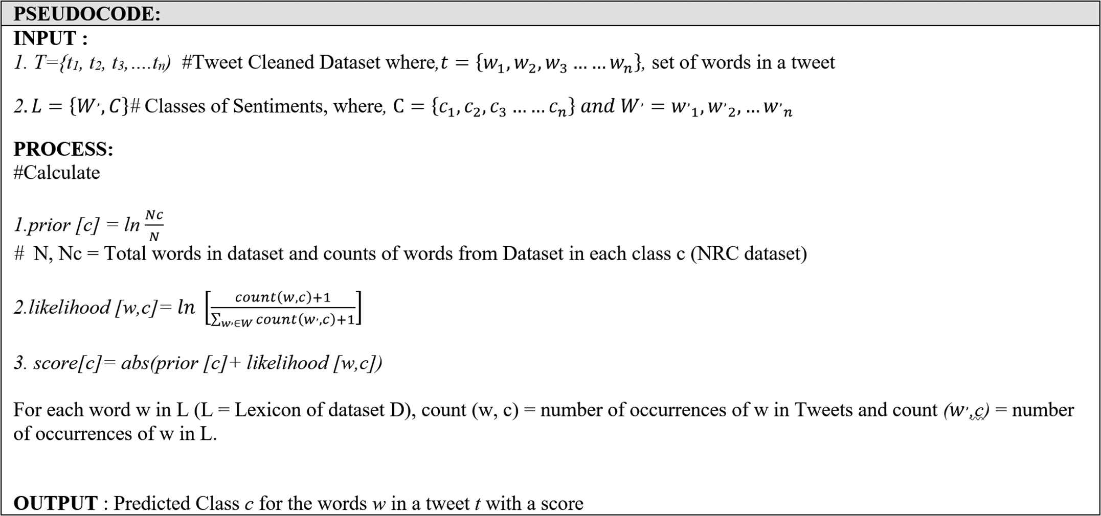
Algorithm for assigning score to the word class.
If the tweet does not have the identical word that exists in the lexical dictionary, then the likelihood in Eq. (6) will be zero as shown in Eq. (7) and this cannot be conditioned, therefore, Laplace smoothing [26] is introduced by adding 1 illustrated in Eq. (8).
While applying this equation in programming, a problematic condition could ascend when count of terms increases. As we know that each probability value of term
The value of probability lies between 0 and 1, whereas log-probability can lie between –∞ and 0.
The log-probabilities are easily comparable between smaller and larger numbers, that argmax does in probabilities for example
Arithmetic works well, i.e., logarithm of the multiplication of the variable is the addition of the logarithms, i.e.,
Logarithmic representation of the Eq. (4) is represented below comprehensively with the final Eq. (9).
Algorithm presented in Figure 2 assigns score to a word according to its frequency that matches with the words in a lexical dataset. The final score is the absolute of addition of logarithmic calculation of prior and likelihood as shown in Eq. (10). So, the algorithm assigns the class score for all words in a tweet. And, we are interested to know if the given tweet, which is as a whole sentence or statement, is whether positive or negative. Therefore, a new metrics “Best fit” is used for categorizing the tweets as “Positive” or “Negative.”
“Best fit” metrics for a given tweet is calculated as the ratio of the scores of positive and negative class as illustrated in Eq. (11). Classes for a given tweet will be assigned based of the conditions of score shown in Table 4. That is, if the value of “Best fit” score is greater than 1, then the tweet is positive; if it is less than 1 then it will be categorized as “Negative” tweet; and if the score is equal to 1, then it will be categorized as “Neutral” tweet.
| Best Fit | Tweet |
|---|---|
| Greater than 1 | Positive |
| Less than 1 | Negative |
| Equal to 1 | Neutral |
Best fit criteria.
3.5. Forecasting Model
This research study uses Exponential forecasting (EF) as a base model for forecasting the sales quantity. Exponential smoothing is a well-known forecasting method and was introduced by [28] and [29]. It can be used as an alternative to group of ARIMA models [30]. EF model equation is shown in the Eq. (12):
Sales data of fashion garment industry was aggregated weekly and an EF was performed. “Corrective Coefficient (Vs)” was calculated, which represents the variation in sales as shown in Eq. (13). Vs is used as an output variable for FSIS, mapping the impact of tweets optimizing the predicting ability of the forecast model.
3.6. Modelling Tweet’s Sentiment Uncertainty for Predicting Sales Using Fuzzy Theory
This section discusses, in detail, the process involved in modelling tweet sentiments. This section is divided into two sub-sections briefing the details of model design and defines linguistic variables for analyzing the impact of Tweet sentiments. Section 3.6.1 outlines the architecture of FSIS model and section 3.6.2 explains the fuzzy linguistic variables for the FSIS model.
The uncertainty is represented by fuzzy sets in classical theory and each element in a set hold a membership degree [31–33]. Fuzzy set can be denoted as a pair
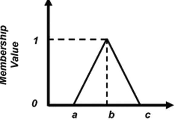
Triangular membership.
3.6.1. FSIS architecture
FSIS architecture is defined using classical “Mamdani” Fuzzy inference proposed by [32,37], the first control system base, fashioning it by if-then rules, which can be gained from human knowledge. This work was inspired by [31] and realized its application of fuzzy inference for complex decision mechanism. Mamdani inference maps the input attributes to the output using fuzzy logic inference which involves steps as follows;
First step involves defining the input and output linguistic variables followed by defining membership function for each linguistic variables
Fuzzification—In this step, input parameters are mapped to appropriate linguistic variables based on pre-defined membership function that can be viewed as fuzzy set. Membership functions are linked with the weight factors that regulate the influence for each defined rule.
Knowledge base—It has a database of fuzzy set and defined rules. “Facts” are symbolized through linguistic variables and reasoning is followed by defined if-then rules.
Inference Engine—Rule inference is managed by inference engine, where human knowledge can be combined without any difficulty using linguistic rules.
Defuzzification—Aggregation of all fuzzy sets to give the single output to draw a conclusion. Centroid method is used for obtaining the crisp number as shown in Eq. (15).
Model design of FSIS involves above steps and this is explained in Section 3.6.2 with input parameters as sentiments and output parameter as corrective coefficient as explained in the Section 3.5, and corresponding defined membership functions.
3.6.2. Defining universal and fuzzy set for sentiments for FSIS
For formalizing and modeling twitter data with garment sales performance, we used intelligent fuzzy technique as discussed in the Section 3.6.1. FSIS constitutes three fuzzy sentiment input variables I as Sp(Positive), Sn(Negative), Sne(Neutral)and Output O as Vs (Corrective coefficient). Triangular membership function is assigned to input variables in the range between [0 1] and output variable in the range [−25 25]. Aggregated weekly sentiment data were used for all three input variables to feed into model. The key objective in modelling sentiments, viz., Sp(Positive); Sn (Negative); and Sne(Neutral)retrieved from tweets with fuzzy inference is to capture human emotions on social media weekly and to forecast the sales variation based on these consumer emotions. Human emotions are uncertain and they change from time to time. So, for example, maybe in one week, sentiment “Positive” could be high and it could lead to a positive effect on sales of upcoming week. Similarly, if it is “Negative,” then it could lead to a negative impact on sales of upcoming week. The designs of the linguistic variables for sentiments are taken as “Low,” “Medium” and “High.” Thus, I is a set of sentiments, i.e.,
Triangular membership function for the input variable in set I is defined between limit [0 1] and the output variable in the limit [−25 25], which is a corrective coefficient in percentage of sales and it will predict sales variation from −25% to 25%. (Table 5 describes) the membership variables and values for the I and O respectively are shown in Table 5. Figures 4 and 5 depict the triangular membership function for variables I and O.
| Input/Membership | Low | Medium | High |
|---|---|---|---|
| (Sp)w | |||
| (Sn)w | |||
| (Sne)w |
| Output/Membership | Low | Medium | High |
|---|---|---|---|
| (Vs) w+1 |
Membership function for input variable I (Input) and O (Output).
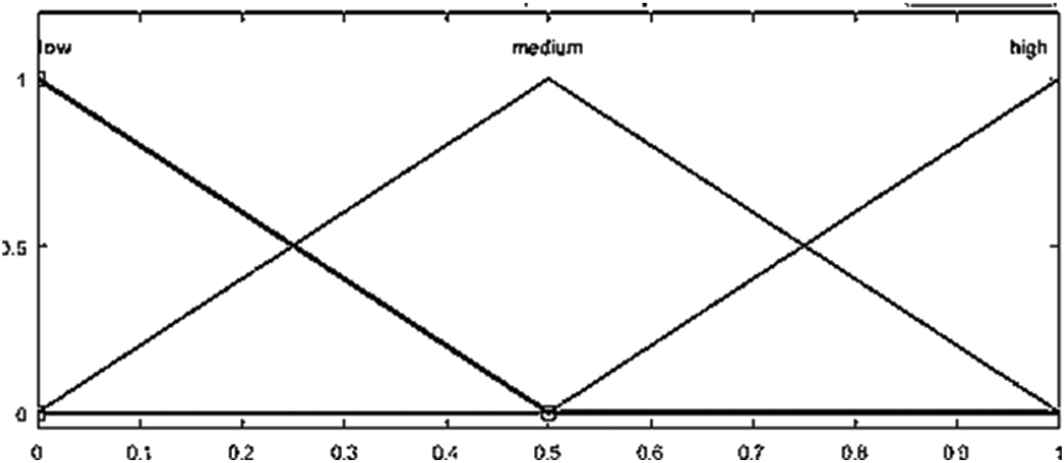
Triangular membership for input variables (Sp, Sn, Sne).
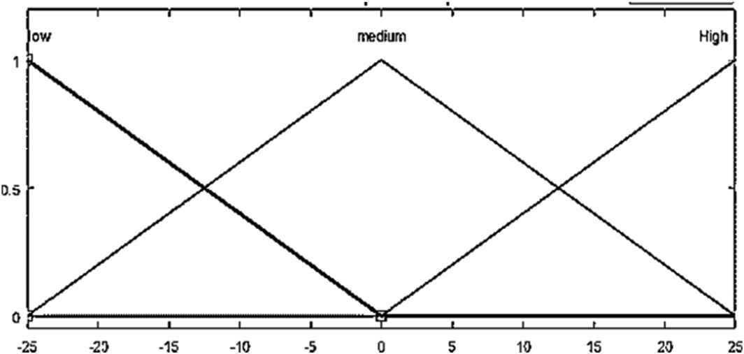
Triangular membership for output variables (Vs).
Calculation of the membership function value for the Input variable “
Similarly, membership function values is calculated for Sn and Sne. Besides, the membership function value for corrective coefficient “
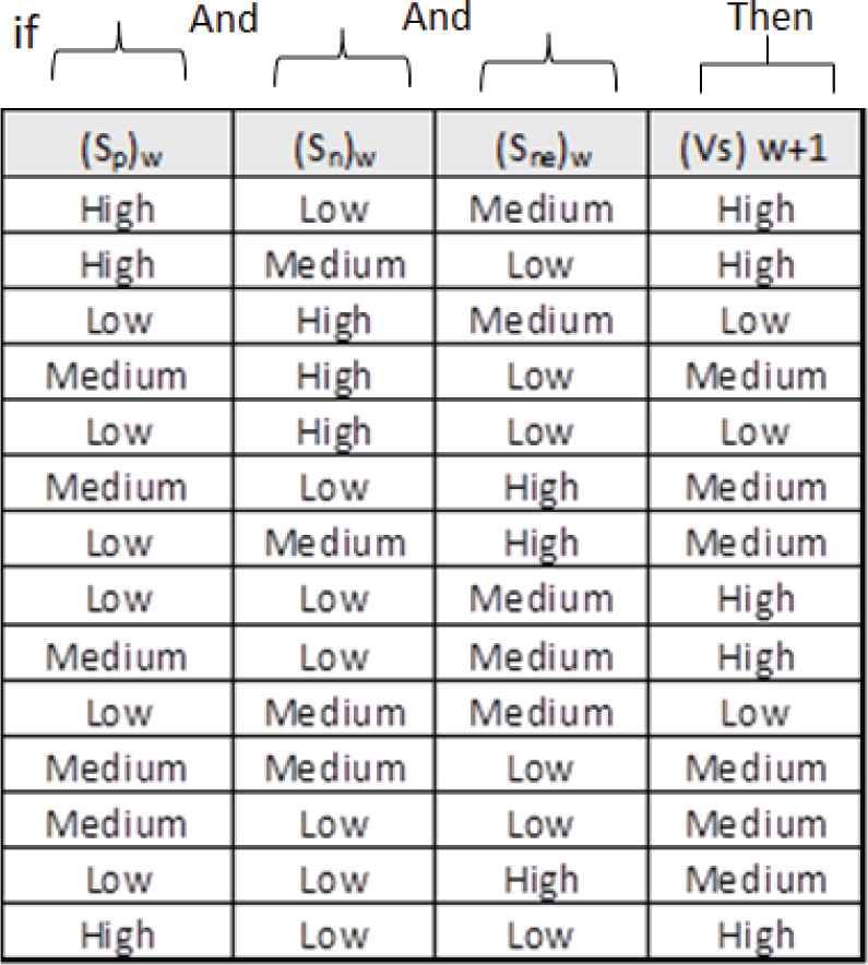
Considering the impacts of the weekly sentiments, fourteen conditional rules are defined by taking into account human knowledge as shown in Table 5. These rules are defined as
“Rule i: IF condition i THEN action I”
To demonstrate the functioning mechanism of rules consider first row of the Table 6, which states that if Sp = High, Sn = low and Sne = Medium, then Vs = High, i.e., if the aggregated weekly positive sentiment is high, negative sentiment is low, and the neutral sentiments is medium, then the sales performance will be high and its values will lie between 0 % to 25 % range, meaning there is an incremental variation in sales than the previous week. Similarly, expected sales variation decision will be taken by the model considering the inference of input variables and defined rules. The final score of the output, i.e., defuzzification of the fuzzy set and the crisp number is calculated by the centroid method using Eq. (15). Architecture of FSIS is depicted in Figure 6.
 |
Rules defined for Fuzzy Sentiment Impact on Sales (FSIS).
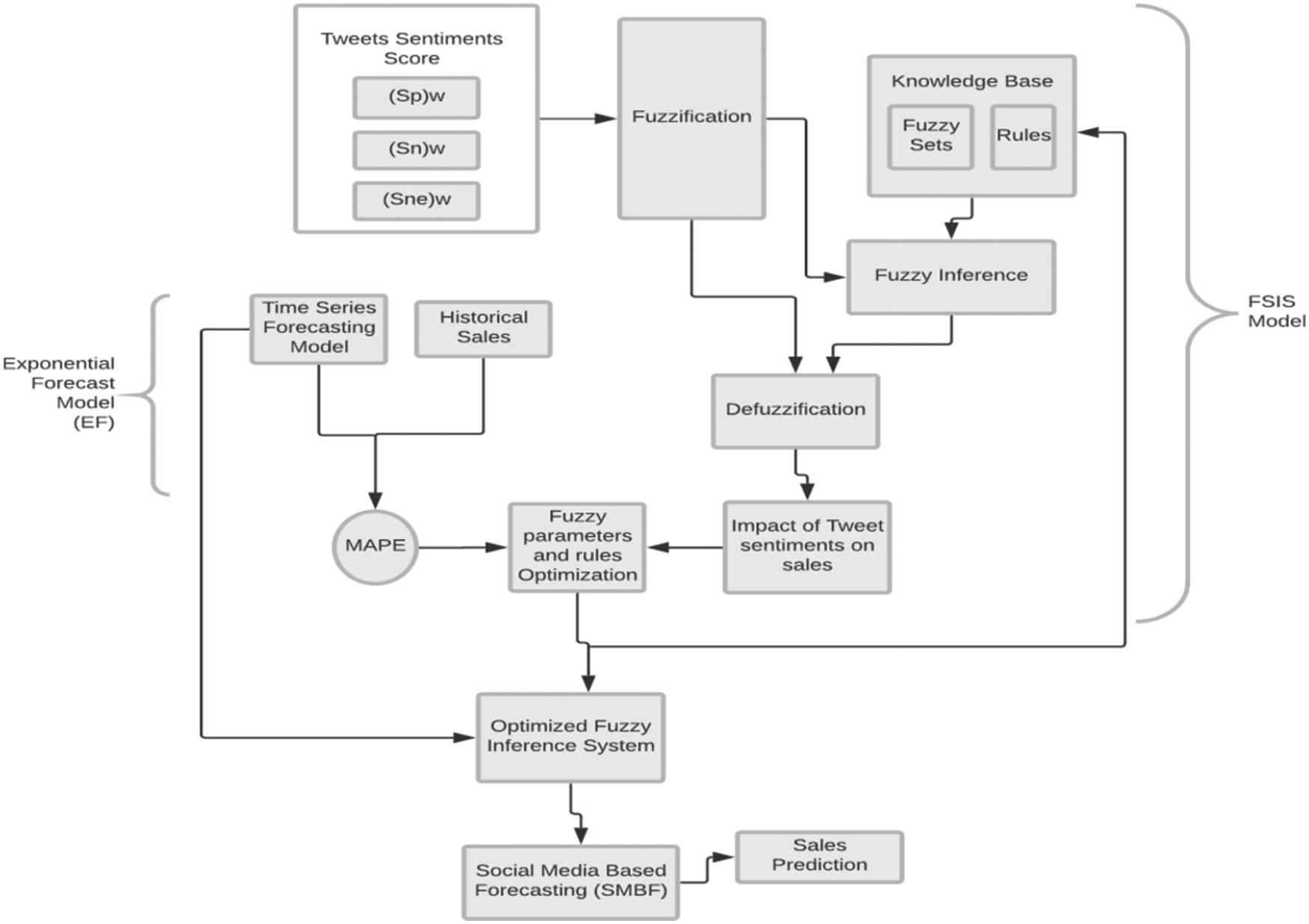
Social Media Based Forecasting (SMBF) model.
3.7. SMBF Model
SMBF model is a time series model, which takes into account the impact of sentiments on sales using FSIS. Parameters of the FSIS are optimized to improve the forecast ability of the model and it is implemented on the exponential time series forecasting and the formula its forecast estimate is given in Eq. (16), where Vs is corrective coefficient, calculated using Eq. (13) and EF is sales volume forecasted by the EF model as explained in section 3.5.
SMBF = sales Forecast from fuzzy time series model
Vs = corrective coefficient predicted by the FSIS model
EF = sales forecasted by Exponential Model
FSIS model parameters, i.e., “Input,” “Output” and “Rules” defined in Section 3.6.2 were optimized using the local optimization method known as “pattern search method” [38], which is useful for the fast convergence. The model was tuned for 500 iterations, and as a result, model was optimized. Optimized parameters for “Input” and “Output” variables are shown in Table 7 and optimized rules are shown in the Table 8.
| Input/Membership | Low | Medium | High |
|---|---|---|---|
| (Sp)w | |||
| (Sn)w | |||
| (Sne)w |
| Output/Membership | Low | Medium | High |
|---|---|---|---|
| (Vs) w+1 |
FSIS, Fuzzy Sentiment Impact on Sales.
Optimized model parameter of FSIS.
| (Sp)w | (Sn)w | (Sne)w | (Vs)w+1 |
|---|---|---|---|
| High | Medium | Medium | High |
| High | Medium | High | High |
| High | High | - | High |
| - | High | Medium | Low |
| High | High | High | Low |
| Medium | Low | High | Medium |
| High | High | Medium | Medium |
| High | Low | Medium | High |
| Medium | Low | Medium | High |
| Low | - | Low | Low |
| - | Medium | Low | Medium |
| High | High | Low | Medium |
| Low | Low | High | Medium |
| Low | High | Low | High |
FSIS, Fuzzy Sentiment Impact on Sales.
Optimized rules defined for FSIS.
3.8. Validation Method and Performance Measure (MAPE)
Mean Absolute Percentage Error (MAPE) is a performance metrics for evaluating the performance of the forecasting models and it is denoted as in Eq. (17).
4. EXPERIMENTAL RESULTS
This section presents the results of all the models discussed in previous section. This section is divided into three subsections: Section 4.1 summarizes the result of NB classifier, which is described in Section 3.4. It is used for extracting sentiments from the tweets and assigning sentiment score to a word in a tweet that matches with the lexical dictionary. Based on sentiment score, tweets are classified as “Positive,” “Negative” and “Neutral” as explained in Section 3.4. Further, in Section 4.2, computational mechanism of correlation between weekly aggregated Twitter sentiments for the current week and sales of the next week is discussed. Lastly, Section 4.3 evaluates the forecast performance of SMBF and EF models.
4.1. Tweet Classification
Tweets were assigned sentiment class as explained in Section 3.4. Logarithmic values of “Prior” and “Likelihood” were calculated of the lexicon dataset [24] and it is shown in the Table 9. The total count of the words labeled “Positive” is 2312 and “Negative” is 3324 in lexical dataset. (To see in detail) Detailed mechanism (of how the) of algorithm is explained in section 3.4. (Let us take one) Consider, for example, in a tweet, “style made genuine matching lining,” the word “genuine” exists in the lexical database as “Positive,” therefore, the score for this positive word in a tweet will be calculated using Eq. (10). As there is only one positive word that matches with the words in lexical dictionary and not with the negative word in a tweet, the score for the“Positive” class will be calculated by using logarithmic value in Table 9 as “0.891062 + (1*7.74586823) = 8.636929”; and for the “Negative” class, it is “0.528006 + (0*8.1088924156) = 0.528006,” and the final score for the best fit will be calculated using Eq. (11) and the result is shown in Table 10. In Table 10, “5” indicates the tweet number in a Tweeter data T. In this case, as the score is more than 1, the assigned class for this tweet is “Positive. ” Similarly, all tweets were assigned scores and classified as “Positive,” “Negative” and “Neutral” based on their “Best Fit” score. Overall classification of cleaned tweets is illustrated in the Figure 7, and it can be seen that about 45% tweets were classified as “Positive”; 27% tweets were classified as “Negative” and approximately 28% of tweets were classified as “Neutral.” The classification results indicate that the chosen fashion brand has quite a positive outlook from customer perspectives as only 27% of total tweets were negative.
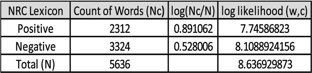 |
Log prior and log likelihood of lexical dictionary.
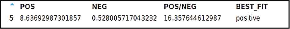 |
Result interpretation for a tweet has one positive word.
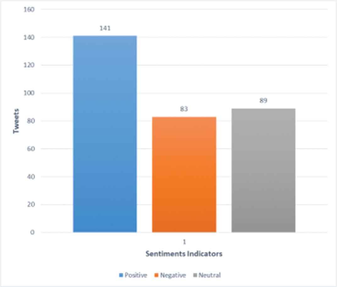
Classification of tweets for fashion brand.
4.2. Correlation Test
The main aim of this study was to investigate if the customer sentiments from tweets collected in the current week have any influence on the upcoming week’s sales. For this, assumption was made and it was verified using Pearson correlation [39]. Following assumptions were made to check the correlation between sentiments indicators Sp, Sn, Sne and sales volume Sv, where Sp= aggregated “Positive” tweets for a week “w,” Sn = aggregated “Negative” tweets for a week “w,” Sne= aggregated Neutral tweets for a week “w,” Sv= Change in volume of sales for week w + 1.
If the correlation between Sp and Sv is positive, then the sales will increase.
If the correlation between the Sn and Sv is negative the sales will be decrease.
If the correlation between the Sne and Sv is positive the sales will be increase.
Correlation values, as shown in the Table 11, indicate that there is a moderate positive correlation between Sne and Sv that is 32%, weak positive correlation between Sp and Sv with a value of 22% and negative correlation between Sn and Sv with −13%. This result clearly shows that if there is more number of positive tweets and neutral tweets, it will have positive effect on sales, whereas if there is more number of negative tweets, it will have negative effect on sales.
| Variables | Correlation |
|---|---|
| Sp and Sv | 0.22 |
| Sn and Sv | −0.13 |
| Sne and Sv | 0.32 |
Correlation table.
4.3. SMBF Model Performance
In this research FSIS is combined and implemented on EF as explained in Section 3.7 and final forecast was achieved by SMBF using Eq. (16). Model performance of SMBF was evaluated by calculating MAPE values as explained in Section 3.8. MAPE values for EF model and SMBF model is shown in the Table 12. This clearly shows that adding the impact of the sentiments by FSIS model on EF model, exhibit the forecasting capability of model. It can be observed that the performance of the SMBF is better than EF, which solely relies on the historical sales information, whereas SMBF model counts on both historical sales data and social media data. This result illustrates that by adding the features of social media in our forecasting model, the performance of the model can be improved significantly.
| Forecasting Model | MAPE |
|---|---|
| EF | 14.7911567205165 |
| SMBF | 10.1143453396686 |
EF, Exponential Forecast; SMBF, Social Media Based Forecasting.
Model evaluation.
The forecasted sales by EF and SMBF models were plotted to compare it with actual sales as shown in Figure 8, which clearly shows that forecast achieved by
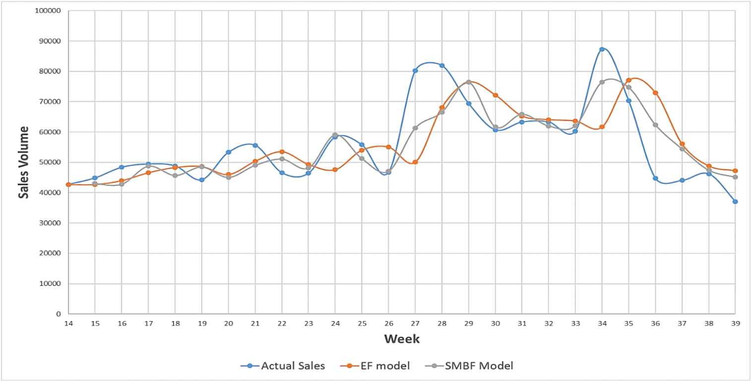
Forecasted sales byExponential Forecast (EF) model and Social Media Based Forecasting (SMBF) model with actual sales.
SMBF model is significantly better than EF. The prediction of the SMBF model was very close to the actual as shown in Figure 8. As the collected data was during summer season, there is a peak in sales for week 27 and 34 while there is a slight drop in week 36. This could be attributed to the promotional or sales discount effect on the sales. These factors are not considered in this study. However, model SMBF tried to capture the trend to some extent.
5. DISCUSSION
This study is conducted on real tweets and sales data of fashion brand for spring and summer assortment. When collected tweets were analyzed after cleaning, the number of tweets was reduced to only 37.5% of the actual tweets in the collected data, which indicates that this brand is in establishing phase on social media. Data pre-processing of tweets was done in two ways: manually; and using text mining to ensure that the collected tweets belonged to the chosen brand. As the enhanced version of lexicon dataset (NRC lexicon) was used, NB classifier classified tweets quite satisfactorily. Most of the tweets were classified as “Positive” and “Neutral,” which represents the popularity of the brand amongst its consumers. This research investigated and established the relationship between the social media data and sales data. Although, the relationship between the social media data and sales data was moderate and weak, we can conclude that there is a relationship between tweet data and fashion apparel sales data, and this indicates that tweet data can be used to forecast garment sales. To deal with the fuzziness of human sentiments and fashion apparel sales, FSIS model was designed, which analyzes the impact of sentiments on sales. FSIS model was combined with EF model to form the SMBF model. The model parameters for SMBF model were optimized using pattern search method used for local optimization reducing the errors between the actual and predicted sales of the model. SMBF model performance is illustrated in Figure 8 and Table 12. SMBF outperforms the EF. There are two peaks in sales for week 28 and week 35, which are summer weeks and model has tried to capture the sales peak during summer to some extent. This shows that the garment sales can be influenced by the social media and if its behavior is modelled in existing time series model, we can considerably improve the performance of the traditional forecasting of garment sales.
6. CONCLUSION AND FUTURE WORK
Taking into account SMBF model performance and results, we conclude that this model could be effective and beneficial to the fashion garment industry. This research proves that social media data can be used for forecasting sales volume. As the forecasting model will be sensitive to social media data, it is the responsibility of a company to increase its visibility on social media in terms of its services and advertisement.
This will improve the quality of collected social media data. The limitation of this study, firstly, lies in the fact that classification of tweets could be improved by adding more words to the dictionary for the class “Positive” and “Negative.” Secondly, as for the presented model, only “Twitter” as a social media data platform was considered, and if we combine other social media platforms such as “Facebook” and “Instagram,” model performance could be enhanced further.
The experiment in this study was focused on weekly forecast, and therefore, overall sales data of a brand was used for analysis. We would like to extend this work in future to create a short term forecasting model to forecast according to the product category. In this experiment, we combined FSIS model with EF model to build SMBF model for forecasting garment sales. In future, we will incorporate other forecasting models to enhance this study further.
CONFLICT OF INTEREST
There is no conflict of interest.
ACKNOWLEDGMENTS
This research work is conducted under the framework of SMDTex-Sustainable Management and Design in Textiles. We are grateful to the company, Evo Pricing, for providing us with the data to carry out this research work.
REFERENCES
Cite this article
TY  - JOUR
AU  - Chandadevi Giri
AU  - Sebastien Thomassey
AU  - Xianyi Zeng
PY  - 2019
DA  - 2019/11/21
TI  - Exploitation of Social Network Data for Forecasting Garment Sales
JO  - International Journal of Computational Intelligence Systems
SP  - 1423
EP  - 1435
VL  - 12
IS  - 2
SN  - 1875-6883
UR  - https://doi.org/10.2991/ijcis.d.191109.001
DO  - 10.2991/ijcis.d.191109.001
ID  - Giri2019
ER  -