
A-SMOTE: A New Preprocessing Approach for Highly Imbalanced Datasets by Improving SMOTE
- DOI
- 10.2991/ijcis.d.191114.002How to use a DOI?
- Keywords
- Imbalanced datasets; SMOTE; Machine learning; Oversampling; Undersampling
- Abstract
Imbalance learning is a challenging task for most standard machine learning algorithms. The Synthetic Minority Oversampling Technique (SMOTE) is a well-known preprocessing approach for handling imbalanced datasets, where the minority class is oversampled by producing synthetic examples in feature vector rather than data space. However, many recent works have shown that the imbalanced ratio in itself is not a problem and deterioration of the model performance is caused by other reasons linked to the minority class sample distribution. The blind oversampling by SMOTE leads to two major problems: noise and borderline examples. Noisy examples are those from one class located in the safe zone of the other. Borderline examples are those located in the neighborhood of the class boundary. These samples are associated with deteriorating performance of the models developed. Therefore, it is critical to concentrate on the minority class data structure and regulate the positioning of the newly introduced minority class samples for better performance of classifiers. Hence, this paper proposes the advanced SMOTE, denoted as A-SMOTE, to adjust the newly introduced minority class examples based on distance to the original minority class samples. To achieve this objective, we first employ the SMOTE algorithm to introduce new samples to the minority and eliminate those examples that are closer to the majority than the minority. We apply the proposed method to 44 datasets at various imbalance ratios. Ten widely used data sampling methods selected from the literature are employed for performance comparison. The C4.5 and Naive Bayes classifiers are utilized for experimental validation. The results confirm the advantage of the proposed method over the other methods in almost all the datasets and illustrate its suitability for data preprocessing in classification tasks.
- Copyright
- © 2019 The Authors. Published by Atlantis Press SARL.
- Open Access
- This is an open access article distributed under the CC BY-NC 4.0 license (http://creativecommons.org/licenses/by-nc/4.0/).
1. INTRODUCTION
Machine learning (ML) techniques are widely used in different applications such as banking, bioinformatics, finance, epidemiology, marketing, medical diagnosis, and meteorological data analysis [1]. In these domains, data is necessary for training the model. However, the distribution of classes in most real-world datasets is imbalanced, and this circumstance poses huge challenge to the standard ML algorithms. The challenge of imbalanced datasets in classification problem arises when the number of samples in one class is far outnumber those of the other class. In such circumstance, a classifier usually favors the majority class in terms of prediction and completely ignores the minority class. This challenge is often experienced in several disciplines when mining data [2]. The consequence of this bias is that, most classification models developed fail to correctly predict the minority class sample in out-of-sample data. This fact is a huge course of worry for real-world data analysis. For example, a software development entity would like to build a classifier to predict whether the software program will have defective modules or not at the end of the development process. In this regard, historical dataset is often employed and the number of fault modules therein is often minimal (i.e., 2%). If a software defect prediction classification model predicts that all the modules are normal (defect-free), it will have a predictive accuracy of 98%. However, the classifier cannot ascertain the target modules that are defective in the dataset. Therefore, if a classifier can efficiently and accurately predict the minority class samples, it will be useful to help several entities make proper decisions and save cost [3,4]. The minority class examples are usually the object of most interest in many applications and the most difficult to predict in the perspective of ML classification task [5,6]. There are several applications including satellite image classification [7], medical applications [8], risk management [9] in which imbalance class distribution is manifested in data. Several works have demonstrated that data mining techniques might not function well when the training data is imbalanced [10]. Conventional ML classifiers assume balanced class distribution for the training data and are predisposed to accurately classify the majority class, whereas the minority samples are often misclassified [11]. The ML community appears to settle on the proposition that class imbalance in training data is a major problem in inductive learning. Although noticed several years back, that imbalance in data may lead to considerable deterioration in standard classification model performance, some scholars have argued that class imbalance in data is not a difficulty itself. In some domains such as the Sick dataset [12] for instance, it has been observed that the standard ML algorithms have the capability to induce effective classification models even when trained on extremely imbalanced data. This illustrates that imbalance class distribution is not the only issue associated with the degradation in performance of classifiers. Also, the classic work of López et al. [13] has demonstrated that the low classification performance reflected in some real imbalanced problems may be associated with the validation scheme applied to evaluate the classifier. A similar view was shared in [14–16] in which the authors are of the view that the deterioration in classification performance is usually associated with other reasons connected to data distributions. Hence, Tang, and Chen [17] proposed an adjustment to the direction of newly created synthetic samples through a mechanism and the empirical results demonstrated improved performance of the classification model built. In that study, oversampling with synthetic samples was presented to minimize overfitting resulting from random and directed oversampling. The new examples were then added into the original training set following specific rules. The aim is to effectively expand the decision zone of the minority class in the feature space, and also augment the number of the minority class samples. However, it is predictable that the addition of new samples in this way will inevitably present further noise into the training dataset, since these synthetic samples generated are no more than a mere estimation of the real distribution [18]. In addition, rare events and class overlapping that come with class imbalance have been identified in [18,19] as potential factors that can result in performance degradation of the model developed on imbalanced data. To further find the possible causes of the learning challenge in imbalanced domain. Prati et al. [20] advanced a methodical research aiming to interrogate whether class imbalances is the main source of hindrance to inductive learning or other factors are responsible for the deficiencies. The study developed on a series of artificial data sets with the view to entirely control all the variables required for the analysis. The experimental results, by applying a discrimination-based inductive framework, demonstrated that the learning challenge is not entirely associated with class imbalance, but is also linked to the level of data overlapping among the classes.
To this end, we propose a critical modification to Synthetic Minority Oversampling Technique (SMOTE) for highly imbalanced datasets, where the generation of new synthetic samples are directed closer to the minority than the majority. In this way, the line of distinction between the two classes will be clearly defined and all samples in data will be located within their class boundaries to ensure accurate prediction of the classifiers developed.
The structure of this paper is organized as follows: Section 2 provides an overview of related works. In Section 3, we present the proposed A-SMOTE. In Section 4, we introduce the experimental results, discuss the evaluation metric and statistical tests used in this work. Finally, concluding remarks and future work are drawn in Section 5.
2. RELATED WORKS
The problem of learning in imbalance domain has been getting attention in different research areas [21–23]. The methods proposed for imbalanced learning can be classified broadly under algorithm level approach and data level approach. In the algorithm level approach, the existing algorithms are modified to recognize samples in the minority class [24]. The drawback of this approach is its dependence on classifiers and the difficulty in handling it [25]. In the data level approach, datasets are modified by adding instances to the minority class or eliminating samples from the majority class. This technique aims to present balanced datasets [26]. The data level technique is easier to use as compared to the algorithm level approach, because the datasets are mended before they are trained by classifiers [27,28]. The main advantage of the data level method is that they are more adaptable since their applications do not dependent on the classifier chosen. Besides, we may preprocess all datasets and apply them to train different classifiers. Among the data level techniques is the well-known SMOTE [23]. In the case of oversampling, SMOTE is applied to introduce synthetic samples along the line segments connecting any or all of the
Extensions of SMOTE by combining it with other techniques such as noise filtering. In the standard classification tasks, noise filters are often used in order to detect and remove noisy samples from training datasets and also to clean up and to create more regular class boundaries [29–31]. Empirical studies, such as [29], confirmed the advantage of integrating iterative partitioning filter (IPF) [32] as a post-processing period after applying SMOTE.
Modifications of SMOTE in which the formation of new minority samples realized by SMOTE is focused on specific portions of the input space, taking the specific features of the data into account. The Safe-Levels-SMOTE (SL-SMOTE) [33], the Borderline-SMOTE (B1-SMOTE and B2-SMOTE) [34] methods come from this category. These methods try to create minority samples close to regions with a high concentration of the minority samples or only within the borders of the minority class.
Ramentol et al. [35] presented a new hybrid approach for preprocessing imbalanced datasets through the creation of new samples, using SMOTE together with the Rough Set Theory. From the experimental results, they observed excellent average results. Similarly, Barua et al. [36] presented MWMOTE to address imbalanced learning problems. The approach first recognizes the hard-to-learn informational minority class samples and assigns them weights based on Euclidean distance from the nearest majority samples and finally creates the synthetic samples from the weighted informational minority samples using a clustering approach. The results showed that their method outperformed other existing methods regarding several estimation metrics, such as AUC and G-mean. Verbiest et al. [37] proposed a hybrid approach FRIPS-SMOTE-FRBPS. First, it cleans data using a fuzzy rough prototype selection technique (FRIPS), that takes the imbalanced characteristic of the data. Second, it uses SMOTE to balance the data and cleans the data again using a fuzzy rough prototype selection technique (FRBPS) for balanced data. Experiments on synthetic data showed that FRIPS-SMOTE-FRBPS outperforms state-of-the-art methods such as SMOTE and its various modifications. Zheng et al. [38] proposed a new oversampling approach SNOCC that can compensate the defects of SMOTE. In this proposed SNOCC, the authors increased the number of seed samples to rule out the new samples from the line segment between two seed samples in SMOTE. Several experiments have been conducted and the results show that new SNOCC performance is higher than SMOTE and CBSO. Among these studies, the effect of noisy and borderline samples on classification model performance in imbalanced data was empirically researched in [16]. Barandela et al. referred to noisy samples as the samples from one class placed inside the area of the other class in [21]. To the best of our knowledge, not enough research attempt has been made to tackle the noise problem and clean borderline examples together on synthetically over-sampled data using SMOTE.
Having this gap in mind, which has not been addressed by many studies, we present a new approach that treats the highly imbalanced dataset following two concepts step by step: Firstly, we create a new synthetic instance using SMOTE algorithm. Secondly, we eliminate the synthetic samples with higher proximity to the majority class than the minority as well as the synthetic instances closer to the borderline crated by SMOTE. Finally, the data is evidently devoid noisy and borderline samples. Details of our new approach for improved classification performance are exhibited in the following sections.
3. SMOTE AND A-SMOTE ALGORITHMS
In this section, we discuss the SMOTE and our A-SMOTE.
3.1. SMOTE: Synthetic Minority Oversampling Technique
SMOTE [23] is an essential approach by oversampling the minority class to generate balanced datasets. It oversamples the minority class by practicing each minority class sample and including synthetic examples along the line segments joining any/all of the
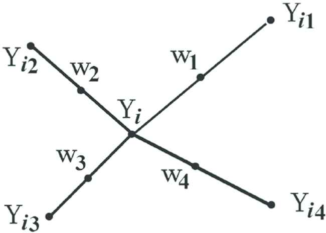
An example of how to generate synthetic data in the Synthetic Minority Oversampling Technique (SMOTE) algorithm.
Synthetic samples generated by taking the difference between the nearest neighbor and feature vector (sample) under consideration. Multiply this difference by a random number among 1 and 0, and add it to the feature vector under consideration. This produces the selection of a random point along the line segment among two distinctive features. The SMOTE algorithm is described in detail below:
Find the k-nearest neighbors for each sample.
Select samples randomly from a k-nearest neighbor.
Find the new samples = original samples + difference * gap (0,1).
Add new samples to the minority. Finally, a new dataset is created.
The SMOTE method comes with some weaknesses related to its insensitive oversampling where the creation of minority samples fails to account for the distribution of sample from the majority class. This may lead to the generation of unnecessary minority samples around the positive examples that can further exacerbate the problem produced for borderline and noisy in the learning process.
3.2. A-SMOTE Algorithm
To perform better prediction, most of the classification algorithms strive to obtain pure samples to learn and make the borderline of each class as definitive as possible. The synthetic examples that are far away from the borderline are more easy to classify than the ones close to the borderline, that pose a huge learning challenge for majority of the classifiers. On the basis of these facts, we present a new advanced approach (A-SMOTE) for preprocessing of imbalanced training sets, which tries to clearly define the borderline and generate pure synthetic samples from SMOTE generalization. Our proposed method has two stages and discussed as follows:
First stage, we first apply SMOTE algorithm to generate the synthetic instance based on following equation:
whereSecond stage, we eliminate the synthetic samples with higher proximity to the majority class than the minority as well as the synthetic instances closer to the borderline generated by SMOTE. The A-SMOTE procedure step-by-step is outlined as follows:
Step 1: The synthetic instances that generated by SMOTE might be accepted or rejected on two conditions and it matches with the first stage: Suppose that
According to Equations (2) and (3), then we get two arrays
Afterwards, we select the minimum value from
To avoid delays caused by the generation of synthetic samples that do not meet the acceptance requirement sequentially and maintain the performance of the algorithm at high speed, in the case of synthetic samples that do not meet the acceptance requirement successively ten times, we accept the synthetic sample of these ten based on its proximity to the minority. This sample is considered as a new synthetic sample and is treated as a sample that meets the acceptance requirement. In this way, we obtain synthetic instances that are near the minority class.
Step 2: After that, with the accepted synthetic instances the following is carried out to eliminate the noisy. Suppose that
whereFor example, if the number of original minority samples is 10, then we choose 10 elements from
Step 3: Similarly, we calculate the distance between
whereThen, we eliminate the half of the synthetic samples that have the least distance between
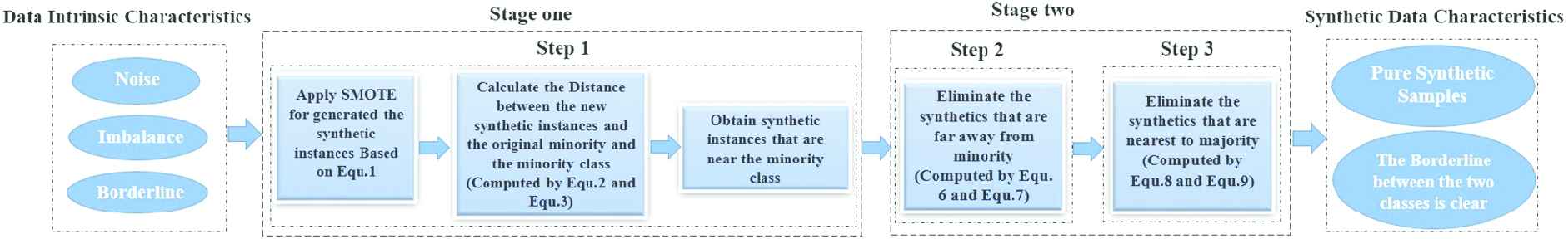
Advanced Synthetic Minority Oversampling Technique (A-SMOTE) algorithm process.
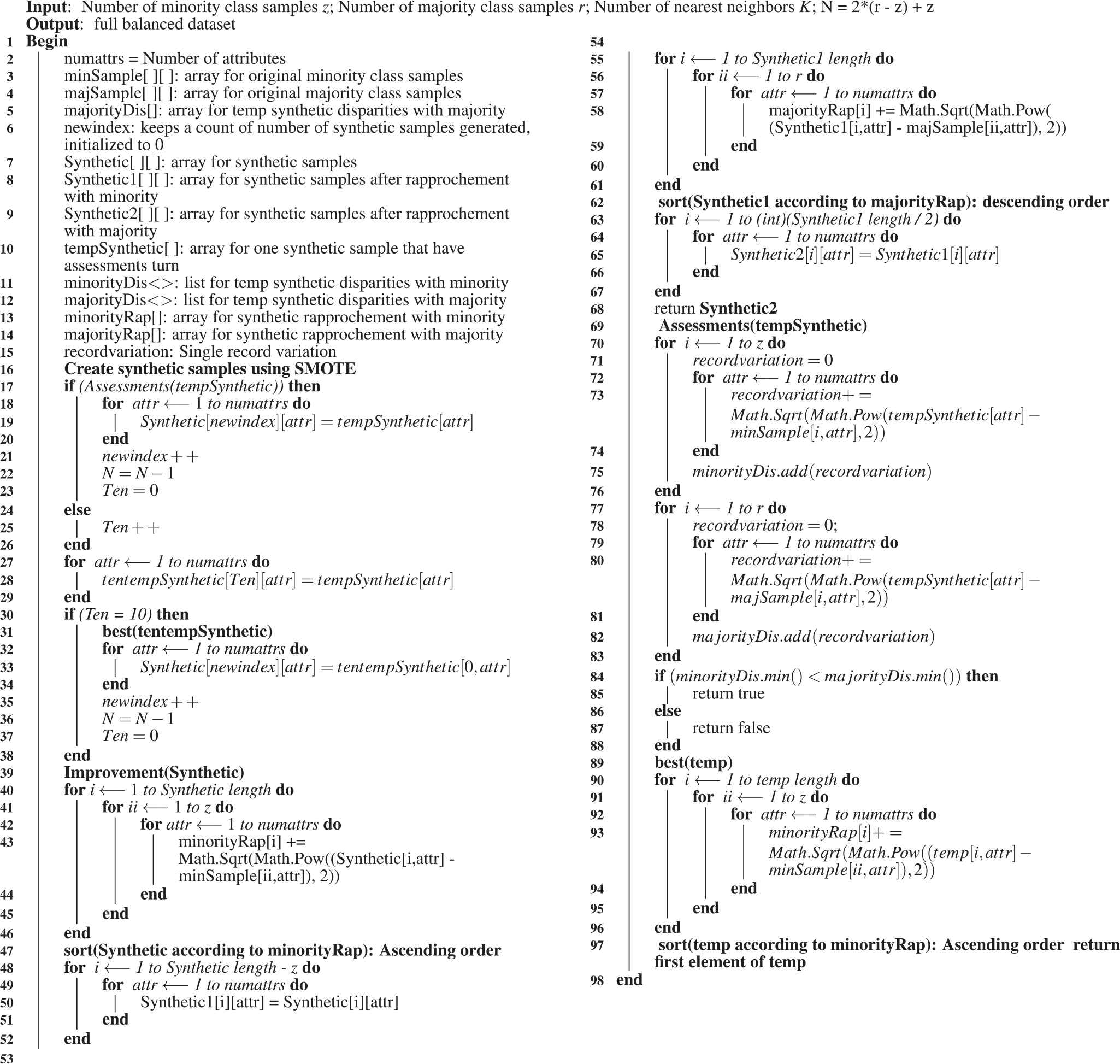
This approach known as A-SMOTE is adopted to design a robust preprocessing method for imbalance learning. The details are illustrated in Algorithm 1.
4. EXPERIMENTAL DESIGN
In this part, we present the experimental design and the results based on the evaluation metrics employed, datasets, different imbalanced methods, and statistical tests. The experiments carried out using Visual Studio 2015, KEEL tool, MATLAB [39], SPSS statistics 22, and RStudio.
4.1. Evaluation Metrics in Imbalanced Domains
It is well known that performance evaluation in imbalanced domains requires the use of individual purpose metrics [40]. In fact, standard performance assessment metrics are focused on the standard behavior instead of the user's preferences which frequently results in misleading conclusions [40,41]. Therefore, when solving problems with imbalanced domains, it is necessary to deal with the issue of performance evaluation. For classification, this point needs more attention but several solutions for evaluation in this context already exist [42]. Therefore, we use confusion matrix to develop multiple evaluation matrix for the purpose of performance evaluation among our proposed method and previous methods. We define the standard rates of accuracy as follows:
Algorithm 1: A-SMOTE Algorithm
When used to evaluate a learner's performance on imbalanced datasets, accuracy is more efficient in the majority class prediction than the minority one. We draw this conclusion from its definition (Equation (10)): if the dataset is unusually imbalanced, even though the classifier proceeds to a correct majority examples classification but misclassifies all the minority examples, the learner still has high accuracy because of the huge amount of the majority examples. In this circumstance, accuracy leads up to an unreliable prediction for the minority class. Thus, in addition to accuracy, more appropriate evaluation metrics must be conducted. The ROC curve [43] is one of the essential metrics to evaluate learners for imbalanced datasets. It is a two-dimensional y and x axis graph where both TP and FP rate are plotted accordingly. The FP rate (Equation (11)) denotes the percentage of misclassified negative examples, and the TP rate (comparison (12)) is the percentage of correctly classified positive cases. Basically, the learners look for the ideal point denoted as (0, 1). The ROC curve highlights trade-offs between benefits (TP rate) and costs (FP rate). To this end, the area under the ROC (AUC) can also be used for the imbalanced datasets evaluation as the following equation shows:
4.2. Datasets and Statistical Tests
In this research, we illustrate the datasets used for the experimental study and the statistical tests used alongside the empirical analysis. We have used 44 datasets from the KEEL data repository1 [44] with highly imbalanced rates. The summary of the datasets appears in Table 1. For our experiments, we admit the following parameters for the A-SMOTE algorithm:
| Dataset | #Instances | #Attributes | %Class (Minority, Majority) | #IR |
|---|---|---|---|---|
| ecoli0137vs26 | 281 | 7 | (2.49, 97.51) | 39.15 |
| shuttle0vs4 | 1829 | 9 | (6.72, 93.28) | 13.87 |
| yeast1vs7 | 459 | 7 | (6.53, 93.47) | 14.3 |
| shuttle2vs4 | 129 | 9 | (4.65, 95.35) | 20.5 |
| glass016vs2 | 192 | 9 | (8.85, 91.15) | 10.29 |
| glass016vs5 | 184 | 9 | (4.89, 95.11) | 19.44 |
| pageblocks13vs4 | 472 | 10 | (5.93, 94.07) | 15.85 |
| yeast05679vs4 | 528 | 8 | (9.66, 90.34) | 9.35 |
| yeast1289vs7 | 947 | 8 | (3.16, 96.84) | 30.5 |
| yeast1458vs7 | 693 | 8 | (4.33, 95.67) | 22.10 |
| yeast2vs4 | 514 | 8 | (9.92, 90.08) | 9.08 |
| Ecoli4 | 336 | 7 | (6.74, 93.26) | 13.84 |
| Yeast4 | 1484 | 8 | (3.43, 96.57) | 28.41 |
| Vowel0 | 988 | 13 | (9.01, 90.99) | 10.10 |
| Yeast2vs8 | 482 | 8 | (4.15, 95.85) | 23.10 |
| Glass4 | 214 | 9 | (6.07, 93.93) | 15.47 |
| Glass5 | 214 | 9 | (4.20, 95.80) | 22.81 |
| Glass2 | 214 | 9 | (7.94, 92.06) | 11.59 |
| Yeast5 | 1484 | 8 | (2.96, 97.04) | 32.78 |
| Yeast6 | 1484 | 8 | (2.49, 97.51) | 39.16 |
| abalone19 | 4174 | 8 | (0.77, 99.23) | 128.87 |
| abalone918 | 731 | 8 | (5.65, 94.25) | 16.68 |
| cleveland0vs4 | 177 | 13 | (7.34, 92.66) | 12.61 |
| ecoli01vs235 | 244 | 7 | (2.86, 97.14) | 9.16 |
| ecoli01vs5 | 240 | 7 | (2.91, 97.09) | 11 |
| ecoli0146vs5 | 280 | 7 | (2.5, 97.5) | 13 |
| ecoli0147vs2356 | 336 | 7 | (2.08, 97.92) | 10.58 |
| ecoli0147vs56 | 332 | 7 | (2.1, 97.9) | 12.28 |
| ecoli0234vs5 | 202 | 7 | (3.46, 96.54) | 9.1 |
| ecoli0267vs35 | 224 | 7 | (3.12, 96.88) | 9.18 |
| ecoli034vs5 | 300 | 7 | (2.33, 97.67) | 9 |
| ecoli0346vs5 | 205 | 7 | (3.41, 96.59) | 9.25 |
| ecoli0347vs56 | 257 | 7 | (2.72, 97.28) | 9.28 |
| ecoli046vs5 | 203 | 7 | (3.44, 96.56) | 9.15 |
| ecoli067vs35 | 222 | 7 | (3.15, 96.85) | 9.09 |
| ecoli067vs5 | 220 | 7 | (3.18, 96.82) | 10 |
| glass0146vs2 | 205 | 9 | (4.39, 95.61) | 11.05 |
| glass015vs2 | 172 | 9 | (5.23, 94.77) | 9.11 |
| glass04vs5 | 92 | 9 | (9.78, 90.22) | 9.22 |
| glass06vs5 | 108 | 9 | (8.33, 91.67) | 11 |
| led7digit02456789vs1 | 443 | 7 | (1.58, 98.42) | 10.97 |
| yeast0359vs78 | 506 | 8 | (9.8, 90.2) | 9.12 |
| yeast0256vs3789 | 1004 | 8 | (9.86, 90.14) | 9.14 |
| yeast02579vs368 | 1004 | 8 | (9.86, 90.13) | 9.14 |
Note: The dataset highlighted in bold also used in Case 2.
Summary of the datasets.
4.3. Comparative Analysis and Results
The experimental findings in this paper are presented using different performance metrics to allow a fair comparison with other methods from the literature among others.
4.3.1. Case 1: Using AUC performance metric
To make a fair comparison, the sets were divided in order to perform a fivefolds cross-validation, 80% for training and 20% for testing, where the 5 test data-sets form the whole set. For each data-set, we consider the average results of the five partitions. The learning algorithm employed for the experiments is C4.5, which has been identified as one of the top algorithms in data mining [48] and has been extensively applied in imbalanced problems [49]. In this part, we compare our approach (A-SMOTE) with seven oversampling and undersampling preprocessing techniques based on SMOTE, that is, the SMOTE algorithm and the preprocessing approaches: S-ENN, S-TomekLinks, Borderline-1, Borderline-2, safelevel, SMOTE-RSB (they are analyzed in [35,50]) and MWMOTE. Table 2 shows the results of the experimental evaluation for the implementation test, wherein the first column we have involved the effect on the datasets, and the best approach is emphasized in bold for each dataset. The performance of the algorithms is ranked on each dataset selected for this study. Thus, our proposed algorithm appears in first place 35 times and five times in the second position. We can recognize that our method obtains the highest performance value of all the methodologies that are being compared. SMOTE-RSB and Borderline-2 achieve good results. Additionally, the unlimited results for SMOTE-ENN and SMOTE-TomekLinks highlight the significance of the cleaning step in the oversampling producing a preferred performance at the classification as compared to SMOTE (see Figure 3). The highest AUC value is shown in Table 3. There are two numbers per cell. The initial number denotes the count of times that a given algorithm is the most preferred over the other algorithms, while the next one shows the number of times shares equal performance with other algorithms.
| Dataset | Original | SMOTE | SMOTE-TL | S-ENN | Border-1 | Border-2 | Safe-level | SMOTE-RSB* | MWMOTE | A-SMOTE |
|---|---|---|---|---|---|---|---|---|---|---|
| ecoli0137vs26 | 0.7481 | 0.8136 | 0.8136 | 0.8209 | 0.8445 | 0.8445 | 0.8118 | 0.8445 | 0.7795 | 0.9648 |
| shuttle0vs4 | 0.9997 | 0.9997 | 0.9997 | 0.9997 | 0.9997 | 0.9997 | 0.9988 | 1 | 1 | 1 |
| yeast1vs7 | 0.6275 | 0.7003 | 0.7371 | 0.7277 | 0.6422 | 0.6407 | 0.6621 | 0.8617 | 0.5669 | 0.8929 |
| shuttle2vs4 | 1 | 0.9917 | 1 | 1 | 1 | 1 | 1 | 1 | 0.9960 | 1 |
| glass016vs2 | 0.5938 | 0.6062 | 0.6388 | 0.6390 | 0.5738 | 0.5212 | 0.6338 | 0.6376 | 0.6905 | 0.8005 |
| glass016vs5 | 0.8943 | 0.8129 | 0.8629 | 0.8743 | 0.8386 | 0.8300 | 0.8429 | 0.8800 | 0.9262 | 0.9580 |
| pageblocks13vs4 | 0.9978 | 0.9955 | 0.9910 | 0.9888 | 0.9978 | 0.9944 | 0.9831 | 0.9978 | 0.9978 | 0.9934 |
| yeast05679vs4 | 0.6802 | 0.7602 | 0.7802 | 0.7569 | 0.7473 | 0.7331 | 0.7825 | 0.7719 | 0.6312 | 0.8610 |
| yeast1289vs7 | 0.6156 | 0.6832 | 0.6332 | 0.7037 | 0.6058 | 0.5473 | 0.5603 | 0.7487 | 0.5271 | 0.8032 |
| yeast1458vs7 | 0.5000 | 0.5367 | 0.5563 | 0.5201 | 0.4955 | 0.4910 | 0.5891 | 0.6183 | 0.5282 | 0.6452 |
| yeast2vs4 | 0.8307 | 0.8588 | 0.9042 | 0.9153 | 0.8635 | 0.8576 | 0.8647 | 0.9681 | 0.8539 | 0.9753 |
| Ecoli4 | 0.8437 | 0.8310 | 0.8544 | 0.9044 | 0.8358 | 0.8155 | 0.8386 | 0.8544 | 0.8710 | 0.9802 |
| Yeast4 | 0.6135 | 0.7004 | 0.7307 | 0.7257 | 0.7124 | 0.6882 | 0.7945 | 0.7609 | 0.5647 | 0.7538 |
| Vowel0 | 0.9706 | 0.9494 | 0.9444 | 0.9455 | 0.9278 | 0.9766 | 0.9566 | 0.9678 | 0.9351 | 0.9796 |
| Yeast2vs8 | 0.5250 | 0.8066 | 0.8045 | 0.8197 | 0.6827 | 0.6968 | 0.8112 | 0.7370 | 0.5545 | 0.9561 |
| Glass4 | 0.7542 | 0.8508 | 0.9150 | 0.8650 | 0.7900 | 0.8325 | 0.9020 | 0.8768 | 0.9077 | 0.9727 |
| Glass5 | 0.8976 | 0.8829 | 0.8805 | 0.7756 | 0.8854 | 0.8402 | 0.8939 | 0.9232 | 0.9618 | 0.9975 |
| Glass2 | 0.7194 | 0.5424 | 0.6269 | 0.7457 | 0.7092 | 0.5701 | 0.6979 | 0.7912 | 0.6661 | 0.8589 |
| Yeast5 | 0.8833 | 0.9233 | 0.9427 | 0.9406 | 0.9118 | 0.9219 | 0.9542 | 0.9622 | 0.8043 | 0.9450 |
| Yeast6 | 0.7115 | 0.8280 | 0.8287 | 0.8270 | 0.7928 | 0.7485 | 0.8163 | 0.8208 | 0.6589 | 0.8745 |
| abalone19 | 0.5000 | 0.5202 | 0.5162 | 0.5166 | 0.5202 | 0.5202 | 0.5363 | 0.5244 | 0.5137 | 0.5630 |
| abalone918 | 0.5983 | 0.6215 | 0.6675 | 0.7193 | 0.7216 | 0.6819 | 0.8112 | 0.6791 | 0.5949 | 0.7672 |
| cleveland0vs4 | 0.6878 | 0.7908 | 0.8376 | 0.7605 | 0.7194 | 0.7255 | 0.8511 | 0.7620 | 0.7158 | 0.9028 |
| ecoli01vs235 | 0.7136 | 0.8377 | 0.8495 | 0.8332 | 0.7377 | 0.7514 | 0.7550 | 0.7777 | 0.7806 | 0.9257 |
| ecoli01vs5 | 0.8159 | 0.7977 | 0.8432 | 0.8250 | 0.8318 | 0.8295 | 0.8568 | 0.7818 | 0.9567 | 0.9779 |
| ecoli0146vs5 | 0.7885 | 0.8981 | 0.8981 | 0.8981 | 0.7558 | 0.8058 | 0.8519 | 0.8231 | 0.8980 | 0.9783 |
| ecoli0147vs2356 | 0.8051 | 0.8277 | 0.8195 | 0.8228 | 0.7465 | 0.8320 | 0.8149 | 0.8154 | 0.8083 | 0.9180 |
| ecoli0147vs56 | 0.8318 | 0.8592 | 0.8424 | 0.8424 | 0.8420 | 0.8453 | 0.8197 | 0.8670 | 0.8173 | 0.9471 |
| ecoli0234vs5 | 0.8307 | 0.8974 | 0.8920 | 0.8947 | 0.8613 | 0.8586 | 0.8700 | 0.9058 | 0.9490 | 0.9691 |
| ecoli0267vs35 | 0.7752 | 0.8155 | 0.8604 | 0.8179 | 0.8352 | 0.8102 | 0.8380 | 0.8227 | 0.7941 | 0.9510 |
| ecoli034vs5 | 0.8389 | 0.9000 | 0.9361 | 0.8806 | 0.8806 | 0.9028 | 0.8306 | 0.9417 | 0.9085 | 0.9765 |
| ecoli0346vs5 | 0.8615 | 0.8980 | 0.8703 | 0.8980 | 0.8534 | 0.8838 | 0.8520 | 0.8649 | 0.8255 | 0.9591 |
| ecoli0347vs56 | 0.7757 | 0.8568 | 0.8482 | 0.8546 | 0.8427 | 0.8449 | 0.7995 | 0.8984 | 0.8445 | 0.9539 |
| ecoli046vs5 | 0.8168 | 0.8701 | 0.8674 | 0.8869 | 0.8615 | 0.8892 | 0.8923 | 0.9476 | 0.8113 | 0.9564 |
| ecoli067vs35 | 0.8250 | 0.8500 | 0.8125 | 0.8125 | 0.8550 | 0.8750 | 0.7950 | 0.8525 | 0.8253 | 0.9302 |
| ecoli067vs5 | 0.7675 | 0.8475 | 0.8425 | 0.8450 | 0.8875 | 0.8900 | 0.7975 | 0.8800 | 0.9528 | 0.9780 |
| glass0146vs2 | 0.6616 | 0.7842 | 0.7454 | 0.7095 | 0.6565 | 0.6958 | 0.7465 | 0.7978 | 0.6402 | 0.8287 |
| glass015vs2 | 0.5011 | 0.6772 | 0.7040 | 0.7957 | 0.5196 | 0.5817 | 0.7215 | 0.7065 | 0.6577 | 0.7723 |
| glass04vs5 | 0.9941 | 0.9816 | 0.9754 | 0.9754 | 0.9941 | 1 | 0.9261 | 0.9941 | 0.9741 | 0.9941 |
| glass06vs5 | 0.9950 | 0.9147 | 0.9597 | 0.9647 | 0.9950 | 0.9000 | 0.9137 | 0.9650 | 0.9258 | 0.9904 |
| led7digit02456789vs1 | 0.8788 | 0.8908 | 0.8822 | 0.8379 | 0.8908 | 0.8908 | 0.9023 | 0.9019 | 0.9212 | 0.9413 |
| yeast0359vs78 | 0.5868 | 0.7047 | 0.7214 | 0.7024 | 0.6228 | 0.6438 | 0.7296 | 0.7400 | 0.5613 | 0.7426 |
| yeast0256vs3789 | 0.6606 | 0.7951 | 0.7499 | 0.7817 | 0.7528 | 0.7644 | 0.7551 | 0.7857 | 0.7137 | 0.8664 |
| yeast02579vs368 | 0.8432 | 0.9143 | 0.9007 | 0.9138 | 0.8810 | 0.8901 | 0.9003 | 0.9105 | 0.8361 | 0.9519 |
AUC, area under the ROC; SMOTE, Synthetic Minority Oversampling Technique.
Illustration of the AUC results for nine preprocessing algorithms using C4.5 classifier (Case 1).
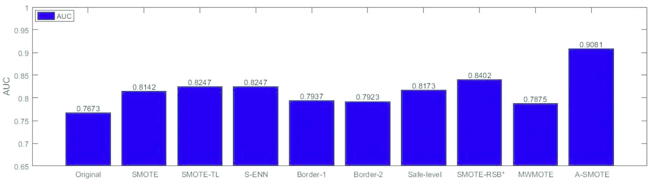
Average area under the ROC (AUC) for 44 datasets and 9 preprocessing technique using C4.5 classifier (Case 1).
| Original | SMOTE | SMOTE-TL | S-ENN | Border-1 | Border-2 | Safe-level | SMOTE-RSB* | MWMOTE | A-SMOTE | |
|---|---|---|---|---|---|---|---|---|---|---|
| TEST | 0/3 | 0/0 | 0/1 | 1/1 | 0/3 | 1/1 | 2/1 | 1/3 | 0/2 | 35/2 |
SMOTE, Synthetic Minority Oversampling Technique.
Illustration of the best algorithm (Case 1).
In this section, our approach obtains the best ranking as shown in Table 4. We can see that, the average ranking of the algorithms demonstrate how good a method over the others. This ranking is accomplished by assigning a position to each algorithm depending on its performance with each dataset. The algorithm that achieves the best accuracy on a specific dataset will have the first ranking (value 1); then, the algorithm with the second best accuracy is assigned to rank 2, and so forth. Finally, this task is carried out for all datasets, and then an average ranking is estimated as the mean value of all rankings.
| Algorithm | Ranking |
|---|---|
| A-SMOTE | 1.4773 |
| S-RSB * | 3.7727 |
| S-ENN | 5.1932 |
| SMOTE-TL | 5.2386 |
| SMOTE | 5.5795 |
| Safelevel | 5.6705 |
| Border-2 | 6.5227 |
| Border-1 | 6.7273 |
| MWMOTE | 6.9659 |
SMOTE, Synthetic Minority Oversampling Technique; A-SMOTE, Advanced SMOTE.
Average ranks obtained by each method in the Friedman test for case 1.
Furthermore, for multiple comparisons, we utilize the Holm post hoc test to determine the algorithms that reject the hypothesis of equality concerning a selected control method (see Table 5). The post hoc system allows the comparison of means to know the acceptance at the lowest significance level
| Algorithm | Holm | Hypothesis | |||
|---|---|---|---|---|---|
| 7 | MWMOTE | 8.502959 | 0 | 0.00625 | Reject |
| 7 | Border-1 | 8.133265 | 0 | 0.007143 | Reject |
| 6 | Border-2 | 7.816385 | 0 | 0.008333 | Reject |
| 5 | Safelevel | 6.496049 | 0 | 0.01 | Reject |
| 4 | SMOTE | 6.355214 | 0 | 0.0125 | Reject |
| 3 | SMOTE-TL | 5.827079 | 0 | 0.016667 | Reject |
| 2 | S-ENN | 5.756662 | 0 | 0.025 | Reject |
| 1 | S-RSB* | 3.556103 | 0.000376 | 0.05 | Reject |
SMOTE, Synthetic Minority Oversampling Technique; A-SMOTE, Advanced SMOTE.
Holms table for α = 0.05, A-SMOTE is the control method for case 1.
4.3.2. Case 2: Using F-measure performance metric
In this part of study, we do the threefold process to measure the performance of the classifier learned from the training dataset generated through different oversampling methods. We randomly partition the dataset into threefolds, and each fold holds almost the same proportion of classes as the original datasets. Of the threefolds, only onefold is retained as the validation data for the testing, and the remaining twofolds are employed as training data. The process is then replicated three times, with each of the threefolds applied precisely once as the validation data. The three results from the folds then are averaged to provide the estimation of one test. We employ Naive-Bayes (NB) classifier to evaluate the efficiency of SMOTE, SNOCC, CBSO, and A-SMOTE. This is done for a fair comparison.
We use a Laplace estimator to calculate the prior probability. The Laplace estimator shows excellent performance in Naive-Bayes classification algorithm [38,51]. One extra benefit of using Laplace estimator is that zero probability can be avoided. F-measure for the minority (positive) class is used as the evaluation standard. In this part, we compare our approach A-SMOTE with CBSO, and SNOCC (they are analyzed in [38,52]). The F-measure value of classification for the different oversampling methods is shown in Figure 4. The oversampling technique is given in the column title. The second column titled Normal is the F-value without oversampling. In each row, the most significant F-value is made bold. From the results of the experiments, a comparison is done to find the best preprocessing algorithm (see Table 6). With AUC and F-Measure results, and statistical tests, we observe that our approach (A-SMOTE) is statistically preferred of all compared techniques.
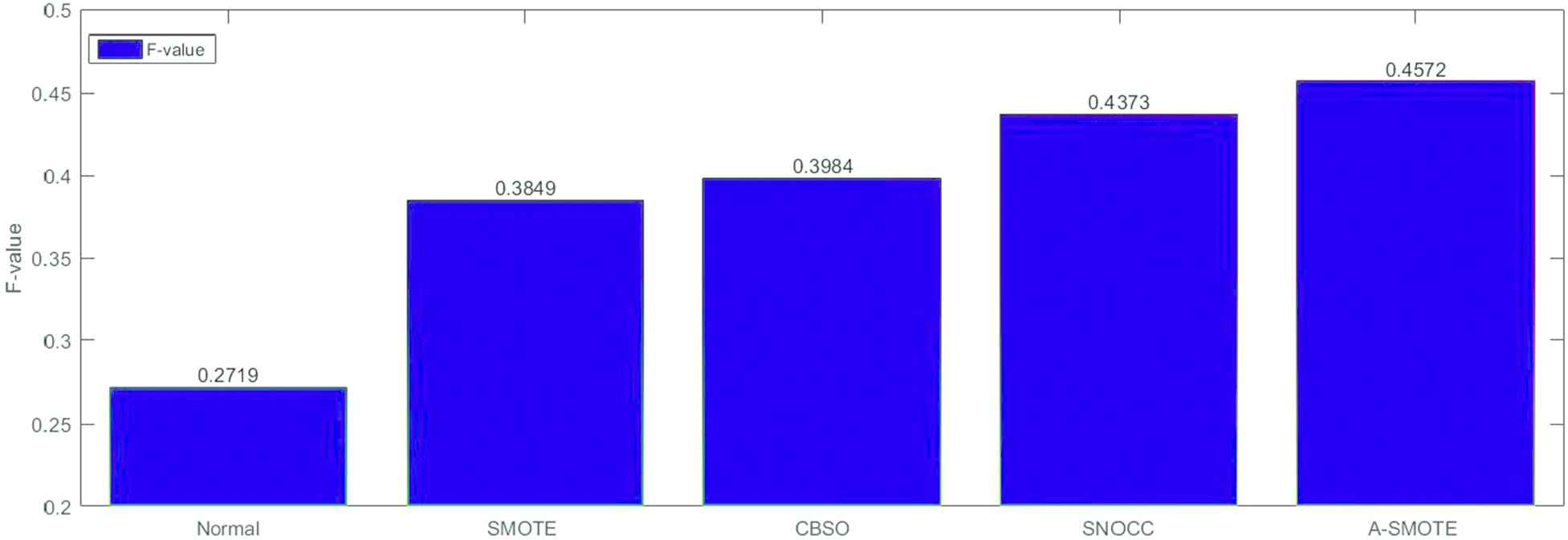
Average F-value for 12 datasets and 4 preprocessing technique using NB classifier(Case 2).
| Data-set | Normal | SMOTE | CBSO | SNOCC | A-SMOTE |
|---|---|---|---|---|---|
| ecoli-0-1-3-7 vs 2-6 | 0.2992 | 0.51 | 0.5028 | 0.5749 | 0.7555 |
| ecoli4 | 0.3626 | 0.6723 | 0.685 | 0.6552 | 0.6336 |
| glass-0-1-6 vs 5 | 0.5597 | 0.562 | 0.6186 | 0.7219 | 0.7903 |
| glass5 | 0.5247 | 0.5407 | 0.5801 | 0.6651 | 0.7115 |
| yeast-0-5-6-7-9 vs 4 | 0.0356 | 0.3272 | 0.3459 | 0.3363 | 0.3621 |
| yeast-1-2-8-9 vs 7 | 0.0265 | 0.083 | 0.0826 | 0.0947 | 0.0990 |
| yeast-1-4-5-8 vs 7 | 0.0091 | 0.1100 | 0.1079 | 0.1286 | 0.1288 |
| yeast-1 vs 7 | 0.1311 | 0.2463 | 0.2365 | 0.2613 | 0.2289 |
| yeast-2 vs 4 | 0.6057 | 0.6739 | 0.6748 | 0.663 | 0.6822 |
| yeast5 | 0.4758 | 0.5279 | 0.5368 | 0.5747 | 0.5404 |
| yeast6 | 0.1882 | 0.2041 | 0.2288 | 0.3903 | 0.3533 |
| yeast4 | 0.0457 | 0.162 | 0.1813 | 0.1818 | 0.2010 |
SMOTE, Synthetic Minority Oversampling Technique; A-SMOTE, Advanced SMOTE.
The F-measure results of different oversampling methods using NB classifier (Case 2).
5. CONCLUSION AND FUTURE WORK
In this study, we have proposed a novel approach for highly imbalanced datasets, A-SMOTE, which is an improvement on SMOTE. The performance of A-SMOTE was evaluated on 44 datasets with high ratios of imbalanced classification. The proposed method was compared with multiple hybrid oversampling and undersampling techniques, using a ML algorithm (e.g., C4.5, Naive-Bayes). In our experimental result, the A-SMOTE technique for preprocessing of imbalanced datasets obtained a higher accuracy and F-measure (F-value). We believe that the proposed A-SMOTE can be a useful tool for researchers and practitioners since it results in the generation of high-quality data. For future work, we will focus on how to combine A-SMOTE with the rough set theory to solve imbalanced datasets classification problem. In addition to that, the problem of imbalanced data has been much related with extended belief rule-based system [53,54] developed to deal with classification tasks. It will have an invaluable contribution in the field of complex data analysis, which we plan to work on in the future.
CONFLICT OF INTEREST
The authors declare no conflict of interest.
AUTHORS' CONTRIBUTIONS
AS. Hussein performed all the experiments, statistical tests, figures, Methodology programming, and writing; T. Li contributed to the supervision, editing, reviewing, and discussion; WY. Chubato and K. Bashir contributed to the debate.
ACKNOWLEDGMENTS
This research was partially supported by Fundamental Research Funds for the Central Universities (No. 2682018CX25).
Footnotes
REFERENCES
Cite this article
TY  - JOUR
AU  - Ahmed Saad Hussein
AU  - Tianrui Li
AU  - Chubato Wondaferaw Yohannese
AU  - Kamal Bashir
PY  - 2019
DA  - 2019/11/28
TI  - A-SMOTE: A New Preprocessing Approach for Highly Imbalanced Datasets by Improving SMOTE
JO  - International Journal of Computational Intelligence Systems
SP  - 1412
EP  - 1422
VL  - 12
IS  - 2
SN  - 1875-6883
UR  - https://doi.org/10.2991/ijcis.d.191114.002
DO  - 10.2991/ijcis.d.191114.002
ID  - SaadHussein2019
ER  -