
An Ensemble Approach for Extended Belief Rule-Based Systems with Parameter Optimization
- DOI
- 10.2991/ijcis.d.191112.001How to use a DOI?
- Keywords
- Extended belief rule base; AdaBoost; Differential evolution algorithm
- Abstract
The reasoning ability of the belief rule-based system is easy to be weakened by the quality of training instances, the inconsistency of rules and the values of parameters. This paper proposes an ensemble approach for extended belief rule-based systems to address this issue. The approach is based on the AdaBoost algorithm and the differential evolution (DE) algorithm. In the AdaBoost algorithm, the weights of samples are updated to allow the new subsequent subsystem to pay more attention to those samples misclassified by pervious system. And the DE algorithm is used as the parameter optimization engine to ensure the reasoning ability of the learned extended belief rule-based sub-systems. Since the learned sub-systems are complementary, the reasoning ability of the belief rule-based system can be boosted by combing these sub-systems. Some case studies about many classification test datasets are provided in this paper in the last. The feasibility and efficiency of the proposed approach has been proven by the experimental results.
- Copyright
- © 2019 The Authors. Published by Atlantis Press SARL.
- Open Access
- This is an open access article distributed under the CC BY-NC 4.0 license (http://creativecommons.org/licenses/by-nc/4.0/).
1. INTRODUCTION
The belief rule-based inference methodology using the evidential reasoning approach (RIMER) proposed by Yang [1] is developed on the basis of Dempster–Shafer theory of evidence [2,3], decision theory [4], fuzzy set theory [5] and traditional IF-THEN rule-based method [6]. This methodology can capture vague, incomplete and uncertain knowledge involved in the dataset to establish a linear or nonlinear relationship between antecedent attributes and an associated consequent. The belief rule-based (BRB) system centered on RIMER is a more generalized expert system. To facilitate a more comprehensive presentation of vague, incomplete and uncertain knowledge, Liu extended the BRB by embedding the belief distribution in the rule antecedent, which is called extended BRB (EBRB) [8]. Liu also proposed a simple but efficient and powerful method for generating initial EBRB from numerical data directly, which can use the dataset adequately and involve neither time-consuming iterative parameter training procedures nor complicated rule generation mechanisms [8].
In a BRB, there are several types of system parameters including belief degrees, attribute weights and rule weights need to be trained. Yang proposed some optimization models to learn the optimal values of these parameters according to the input and output data [7]. The extended belief rule generation methodology proposed by Liu [8] allows automatically transforming a dataset into an EBRB. It can be seen from the BRB parameter training approaches and the EBRB rule generation mechanism that the dataset plays a vital role in the reasoning performance of BRB or EBRB systems. However, several types of problem may be caused by the dataset, which will lower the reasoning ability of the EBRB system. Over-fitting occurs when an EBRB system fits to the training instances well but fails to provide exact results for the test instances because of the undesirable dataset. In addition, owing to the noise, varied quality or reliability of the dataset, it is likely that inconsistency is common in the data-driven belief rule bases [1,8]. A situation of inconsistency occurs when there are two or more rules with different consequents but exactly similar antecedents are activated simultaneously for the same input. It is worth nothing that the emergence of inconsistency that does not exist in the initial EBRB system may attribute to the parameter training procedure. Some other problems such as poor generalization and reasoning instability may also arise easily due to the lack of training instances or uneven sampling. Therefore, it is highly essential to enhance the reasoning ability of EBRB systems by weakening the negative impacts of above problems caused by dataset.
To boost the reasoning ability of EBRB systems, this paper proposes an EBRB systems ensemble method which is based on the AdaBoost algorithm and uses the DE algorithm as the parameter optimization engine. In the AdaBoost algorithm, the weights of the samples are assigned the same value first and are then updated to learn a serious of sub-models which are tweaked in favor of those samples with high weights. The DE algorithm, as one of the most advanced Evolutionary Algorithms (EAs), is applied in the proposed ensemble method to learn EBRB sub-systems with the lowest error classification rate. Since those samples with high weights, misclassified by previous sub-models, are emphasized in the ensemble method, the negative impacts of the dataset on the reasoning ability of the EBRB system can be reduced gradually. Ultimately, the overall EBRB system, a combination of a series of EBRB sub-systems, is capable of reasoning with higher accuracy. In order to demonstrate the effectiveness of our method, some case studies are provided in this paper.
The remainder of this paper is organized as follows. The EBRB representation, generation and inference procedure are reviewed briefly in Section 2. In Section 3, we propose an AdaBoost-based ensemble method to combine different but complementary EBRB sub-systems to generate an overall system. The efficiency of the proposed ensemble method is validated in Section 4 using some case studies in several benchmark datasets. Conclusions are drawn in Section 5.
2. RELATED WORK
At present, the application of ensemble learning in the whole BRB research field is still in its infancy, and the papers in the field of EBRB are more scarce. Therefore, this paper will not only confine to ensemble learning, but also introduce other models in the field of EBRB classification in recent years. Yang [22] proposes a multi-attribute search framework (MaSF) to reconstruct the relationship between rules in the EBRB to form the MaSF-based EBRB, two methods are used to solve the classification problem of low-dimensional data and high-dimensional data, respectively. Yang's [21] DEA-EBRB model focuses on rule reduction. Data Envelopment Analysis (DEA) is introduced to evaluate the validity of rules and delete invalid rules. When calculating negative individual matching degress, there might appear negative values and all rules' activation weights may be equal to zero. To address this problem, Lin [23] introduces the Euclidean distance which is based on attribute weights and improves the traditional similarity computational formula. Yang [26] propose a novel activation weight calculation method and parameter optimization method to enhance the interpretability and accuracy of the EBRB system. The results indicate that the EBRB-New model prevents counterintuitive and insensitive situations and obtains better accuracies than some studies. Micro-EBRB model proposed by Yang [25] focuses on the efficiency optimization of EBRB system on large-scale data sets, and proposes a simplified evidential reasoning (ER) algorithm and the domain Division-based rule reduction method. The comparative analyses of experimental studies demonstrate that the Micro-EBRBS has the comparatively better time complexity and computing efficiency than some popular classifiers, especially for multi-class classification problems.
3. OVERVIEW OF EBRB
3.1. Extended Belief Rule-Base
The EBRB [8] is summarized firstly in this section, which is extended with belief degrees embedded in the antecedent terms of each rule. And a data-driven approach, a more flexible and simpler rule generation mechanism, was proposed in [8]. Thanks to the new features of the EBRBs, they can represent the vagueness, incompleteness and uncertainty of the dataset more exactly and reflect the potential ambiguity contained not only in the consequent attribute but also in the antecedent attribute.
Suppose an EBRB is constituted by several rules with the
The original BRB system is usually built by the domain experts knowledge while the rule generation methodology presented in [8] provides a mechanism to build an EBRB from the dataset directly without any other information. Suppose that
The belief distributions of antecedents and consequents of the EBRB can be generated from the above equivalent formulas. Note that this type of transformation scheme is suitable for the case of utility-based rule base with extended belief structure. Other detail input transformation schemes can be viewed from [8].
3.2. Extended Belief Rule-Based Inference
The inference of the EBRB is still conjoined with the ER approach, using new individual matching degree calculation formula. The EBRB inference methodology, the new RIMER+, consists of two main processes which are the activation process and the inference process. The activation process refers to calculate the weight of each rule. And the weights of all rules will be aggregated together with the rules' consequents to infer a result in the inference process. Thanks to the new features involved in the representation of the EBRB, a new method to calculate the individual matching degree was proposed by Liu [8]. Considering the belief distribution of antecedent attributes in the
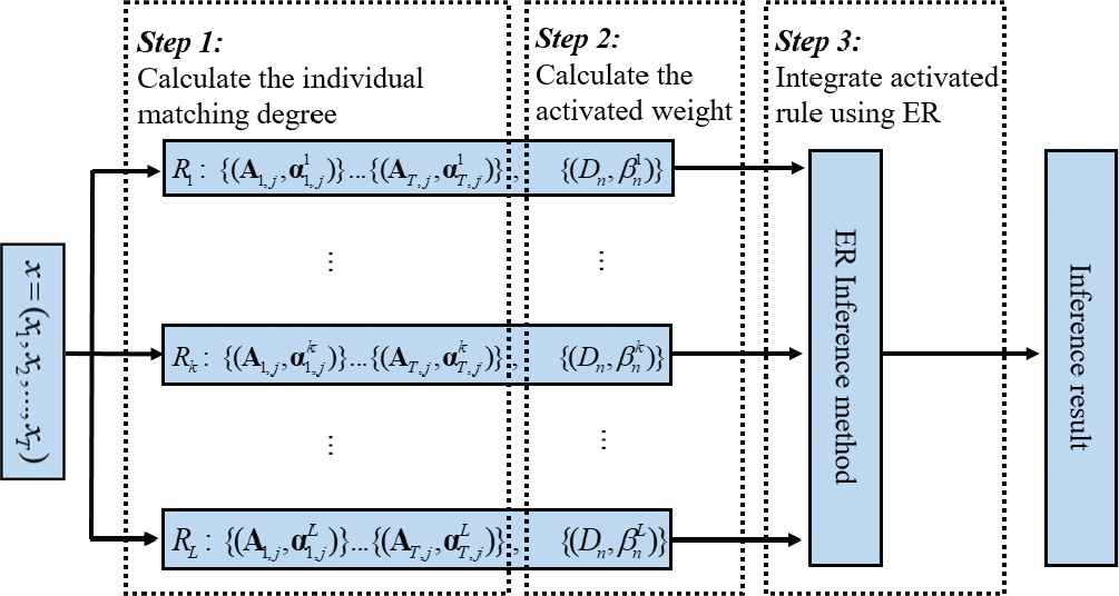
Illustration of inference mechanism.
Once the individual matching degrees are computed, the activation weight of the
Finally, the rule activation weights of all rules in the EBRB can be aggregated using the ER algorithm as inference engine to get an output (Step 3 of Figure 1). For a more detailed description of this process, please see [1].
4. AN ENSEMBLE METHOD FOR THE EXTENDED RULE-BASE
4.1. Ensemble Learning Method
The narrower term ensemble methods refer to the combination of sub-models which learned by the same algorithm. Some popular algorithms that can be used to learn sub-models are the decision tree, the neural network, the support vector machine, etc. While in a broad sense, a combination of multiple sub-models which solve the same problem is exactly an ensemble method. In the initial stage of ensemble methods research, majority literatures [11] focused on narrow ensemble methods. However, as the big data is being paid more and more attention, broad ensemble methods are accepted by more scholars.
The ensemble learning, a hot area in machine learning research, combines a series of sub-models learned by some approaches with a certain criterion to create an improved model. The ensemble learning process can be divided into two steps, first, learning a series of complementary sub-models, second, combine those learned sub-models to get an improved model. The efficiency of ensemble learning is concerned with the diversity of sub-models and therefore it is crucial to learn high disparities but complementary sub-models. Since the learning algorithms in the broad ensemble method are different, the learned sub-models are diverse as well. There are four main approaches to learn different sub-models in narrow ensemble methods as follows:
Training instances processing method. The dataset is partitioned into several independent training instances by a certain approach to learn different sub-models. So far, the most common implementation of this method are bagging and boosting [9].
Input features processing method. Selecting a subset of original input features for use in multiple features problems to learn different sub-models [10].
Output results processing method. A method, converting the multivariate classification into binary classification, was proposed in [13].
Parameters processing method. Common learning algorithm, such the decision tree and the neural network, need to determine the values of parameters. This is because different values of parameters may contribute to entirely different output results.
The finally result of the improved model is obtained by the way of aggregating a series of different results from sub-models. In classification problems, the output information of ensemble learning models can be marked off into three levels as follows [14]:
The abstract level. Each learned sub-model only outputs one classification result.
The rank level. Each learned sub-model outputs all possible classification results which will be sorted by possibility.
The measurement level. Each learned sub-model outputs the measurement values of all results. The measurement values can be represented by probability or belief.
Among the above three levels, the measurement level contains the highest amount of information and the abstract level contains the lowest. Many combination methods are able to combine sub-models, i.e., simple majority vote policy [12,14,15], Bayesian vote policy [14,16], a combination method using the Dempster–Shafer theory of evidence [14,17].
4.2. Differential Evolution Algorithm
The main aim of the AdaBoost algorithm is generating sub-models of which the reasoning ability on those instances misclassified by previous sub-models should be as good as possible. Since the sub-models in this paper are EBRB sub-systems, the values of parameters play a significant role in the reasoning ability of EBRB systems. Therefore, it is necessary to train the parameters of EBRB systems and the DE algorithm is an applicable candidate.
The DE algorithm, simulating biological evolution, is a random iterative algorithm, proposed by Storn and Price in 1995 [18]. Its essence is a multi-objective optimization algorithm, which is used to solve the global optimal solution in multi-dimensional space. It's basic idea is derived from genetic algorithm, which simulates the hybridization, mutation and replication of genetic algorithm to calculate the sub. Through continuous evolution, retaining good individuals, eliminating inferior individuals and guiding search to approximate the optimal solution.
Compared with other EAs, such as the Genetic Algorithm, Particle Swarm Optimization, DE's robustness is good due to its simpler structure, a faster evolving speed and global searching speed.
The main steps of the DE are as follows:
Step 1: Initialization
Initialize the population
Step 2: Mutation
Generate a variation individual according to the following formula:
Step 3: Crossover
Crossover according the following formula:
Step 4: Selection
Calculate the crossed individual's fitness to select a new individual with a higher fitness value. The
After the selection, if the number of iterations is up to the given value
4.3. The Ensemble Method for EBRB Systems
4.3.1. Flow chart of ensemble method for EBRB
Figures 2 and 3 describes the process of the EBRB systems ensemble method which is based on the AdaBoost algorithm and uses the DE algorithm as the parameter optimization engine. The first step required is to initialize all samples to the same weight, then learning the parameters of EBRB sub-systems using the DE algorithm. Note that only the weights of extended rules are trained in this paper. In the process of parameter learning of DE algorithm, the objective function is the weighted misclassification rate of BRB subsystem, the BRB subsystem trained by this method will pay more attention to the data with higher weights. Then, the weights of the samples are updated according to the performance of the learned EBRB subsystem. Repeat above processes unless the number of EBRB sub-systems reach the given value. Ultimately, those EBRB sub-systems with better reasoning ability will be combined to get the final result. Since each learned EBRB subsystem has its own weight, the reasoning result of the test instance is obtained by the weighted voting method.
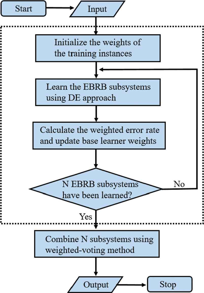
The ensemble method for extended belief rule-base (EBRB).
The ensemble method for extended belief rule-base (EBRB).
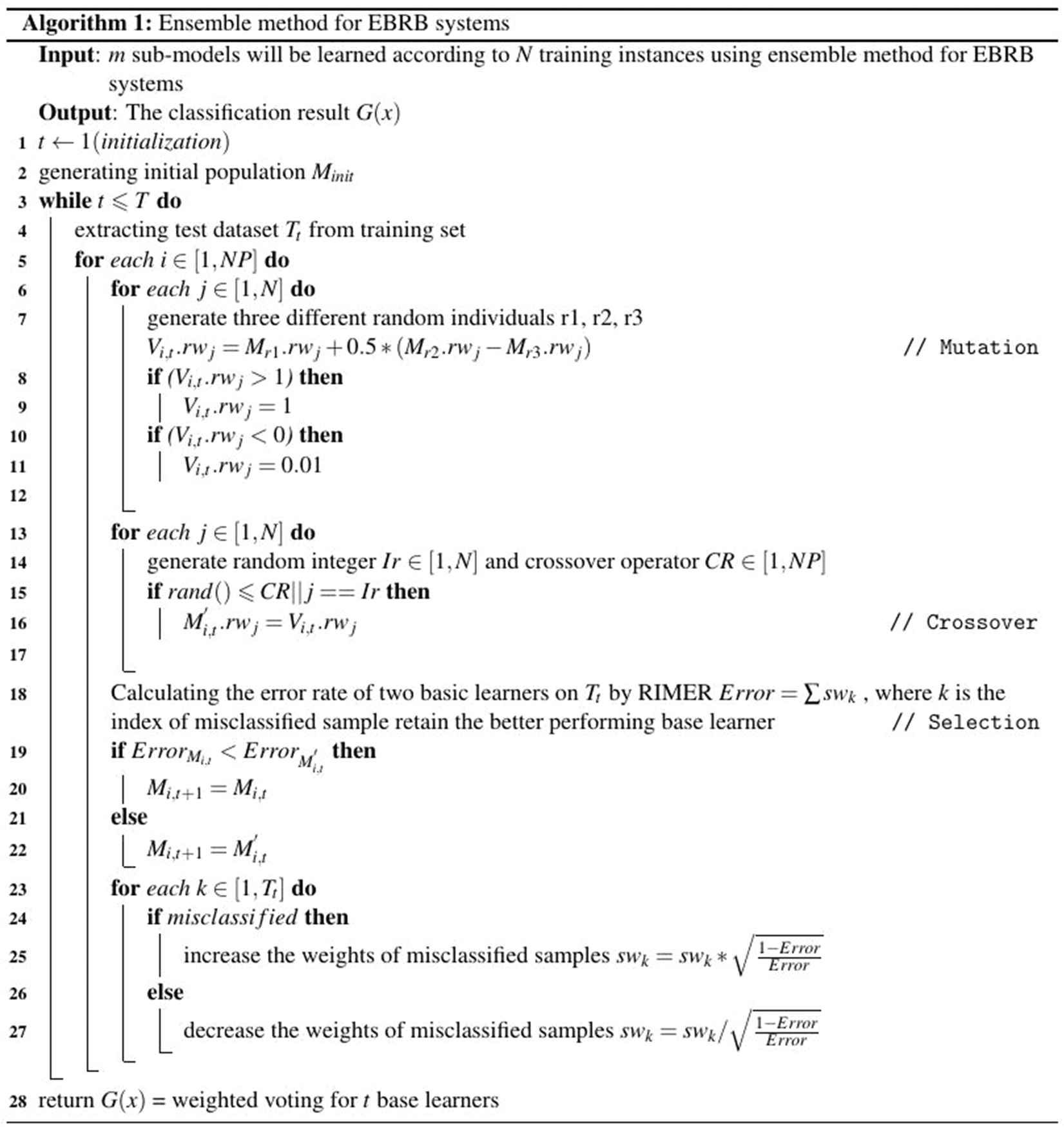
4.3.2. Parameter optimization process based on DE algorithm
Combined with Figure 3, the process of parameter optimization of DE algorithm will be explained in detail below. In the first iteration, the initial population
In the mutation stage, two populations will be randomly selected to perform mutation operation with the original population, resulting in the mutation population
In the crossover stage, the crossover operation between the mutated individual and the original individual will be carried out according to the crossover probability
In the selection stage, the RIMER method and sample weight
4.3.3. Detailed description of AD-EBRB
In order to better explain the model architecture of this paper, the dotted line part of Figure 2 is further explained in detail. It should be noted that this paper does not use the original AdaBoost integrated learning algorithm, but incorporates the idea of this method into the learning process of EBRB sub-systems, that is, by increasing the system's attention to error samples, the EBRB subsystem with better classification performance are generated iteratively. The generation process of the original AdaBoost learner depends on the data, and the differences between the base learners are obtained by different sample weights. The diversity of base learners is an important factor affecting the classification effect, hence differential evolution (DE) algorithm is introduced to increase the diversity of base learners.
As shown in step 1 of Figure 4, the training data generated by the 10-fold cross-section (10-CV) is segmented again, and part of the data is extracted as test set
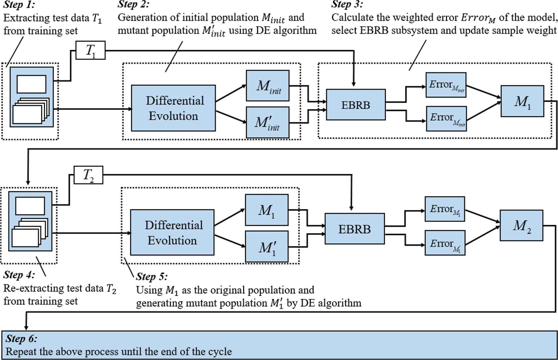
The discription of AdaBoost + differential evolution + extended belief rule-base (AD-EBRB).
In step 2 of Figure 4, the initial population
In step 3 of Figure 4, the weighted error rates of
Step 4 is basically the same as step 1, and test data
5. CASE STUDIES
All datasets used for classification are obtained from the well-known University of California Irvine (UCI) machine learning repository, which contains various types of datasets and is widely used in the testing of various classification models [19]. The dataset information used in this paper is shown in the following table:
In the process of EBRB construction, it is assumed that each antecedent attribute of the dataset contains five evaluation levels, and the number of consequents is consistent with the number of categories in the data. In addition, the 10-CV method is used to divide the dataset into 10 blocks, 9 of which are used to train the EBRB model, and the remaining one is used for testing. Taking Iris dataset as an example, the running process of AdaBoost+DE+EBRB (AD-EBRB) model is introduced. In the first step, five antecedent ratings are used to define four antecedent attributes, these ratings are choose evenly from each antecedent data. and then EBRB rules are generated from training data to construct the initial EBRB system. The corresponding antecedent values for each antecedent attribute are expressed as follows:
Three consequent ratings are applied to describe the three classes as follows:
For 150 Iris data, these data are equally divided into 10 blocks, and the sampling ratio of different classes of data in each dataset is basically the same as that in the original dataset. In each iteration, 9 of the 10 blocks are composed into one training data, and some of them are extracted as test samples in the process of AdaBoost learning. EBRB is constructed using the remaining training data. The initial population (rule weight) is generated by DE algorithm. After crossover and mutation operations, the rule weight in the new population and the old population is regarded as two independent EBRB sub-systems. The output of EBRB subsystem is obtained by ER algorithm, and the weighted error rate is calculated, the data weight and the subsystem weight are updated. The subsystem with lower weighted error rate is selected to continue the next round of DE until the number of base learners reaches the target. Finally, the error of AD-EBRB model is verified by the remaining one-fold test data. The final error rate of the AD-EBRB model is the average of 10-CV.
5.1. The Influence of the Number of EBRB Sub-Systems
Figure 5 shows the number of misclassification samples in the one 10-CV test of the glass dataset using the proposed ensemble method. The horizontal axis is the number of EBRB sub-systems while the vertical axis denotes the number of misclassification samples. It can be seen from Figure 5 that although the number misclassification samples does not decrease monotonously, the overall trend of it takes on a downward trend as the number of EBRB sub-systems increases.
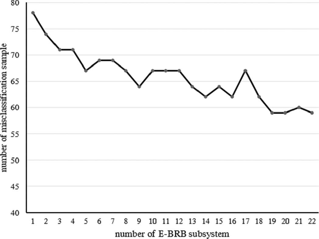
The trends of AdaBoost + differential evolution + extended belief rule-base (AD-EBRB).
In order to verify the applicability of the ensemble learning method of EBRB system in classification problems, the UCI classification data set in Table 1 is used for experiments. In the generation stage of EBRB subsystem, the number of BRB systems is specified: 25, 100 and 200, respectively. Then the ensemble learning method of EBRB system based on AdaBoost and DE algorithm proposed in this paper is compared with other existing methods. Naive Bayes and C4.5 are classical single classifier algorithms. BRBCS-Vote is a method of ensemble learning for BRB system by majority voting method, which also controls 25, 100 and 200 basic learning systems. In this experiment, three different EBRB systems are constructed to analyze and compare the performance of algorithms, including the original EBRB; AD-EBRB-Votes is an EBRB ensemble learning system with different number of base learners, and the combination of the system is simple voting method; AD-EBRB-Votes is also an EBRB ensemble learning system with different number of base learners, and the combination of the system is weighted voting method, the weight referred to here is the weight of each EBRB subsystem.
| No. | Names | Samples | Attributes | Classes |
|---|---|---|---|---|
| 1 | Iris | 150 | 4 | 3 |
| 2 | Hayes-roth | 160 | 4 | 3 |
| 3 | Wine | 178 | 13 | 3 |
| 4 | Glass | 214 | 9 | 6 |
| 5 | Thyroid | 220 | 5 | 3 |
| 6 | Seeds | 210 | 7 | 3 |
| 7 | Ecoli | 336 | 7 | 6 |
| 8 | Bupa | 345 | 6 | 2 |
| 9 | Diabetes | 393 | 8 | 3 |
| 10 | Cancer | 569 | 30 | 2 |
| 11 | Pima | 768 | 8 | 2 |
| 12 | Mammographic | 830 | 5 | 2 |
| 13 | Contraceptive | 1473 | 9 | 3 |
| 14 | Yeast | 1484 | 8 | 10 |
Basic information of classification datasets.
From the Table 2, we can find that on Glass and Iris datasets, the classifier system based on ensemble learning has better classification accuracy than the single classifier system. This shows that the ensemble learning method proposed in this paper can indeed improve the reasoning performance of EBRB system. Because the system combines the AdaBoost ensemble algorithm, the new BRB system can focus on the data of the previous system misclassification, and the differential evolution algorithm is introduced to train the rule weights of the BRB subsystem to ensure the reasoning ability of the BRB subsystem, so that the AdaBoost algorithm can play a role and improve the accuracy of the algorithm.
| Method | Cancer | Glass | Iris | Average |
|---|---|---|---|---|
| Naive Bays | 95.90 (3) | 42.90 (5) | 94.71 (3) | 3.67 (5) |
| C4.5 | 96.00 (2) | 67.90 (2) | 95.13 (4) | 2.66 (3) |
| EBRB | 96.38 (1) | 67.90 (2) | 95.13 (4) | 2.33 (2) |
| BRBCS-Vote (25) | 95.03 (5) | 66.35 (4) | 96.00 (1) | 3.33 (4) |
| BRBCS-Vote (100) | 95.43 | 63.56 | 94.10 | |
| BRBCS-Vote (200) | 93.84 | 61.86 | 84.67 | |
| AD-EBRB-Votes (25) | 95.06 | 68.16 | 95.99 | |
| AD-EBRB-Votes (100) | 95.01 | 69.22 | 95.32 | |
| AD-EBRB-Votes (200) | 94.89 | 67.93 | 95.32 | |
| AD-EBRB-Weights (25) | 95.40 (4) | 72.40 (1) | 96.00 (1) | 2 (1) |
| AD-EBRB-Weights (100) | 95.18 | 70.18 | 95.92 | |
| AD-EBRB-Weights (200) | 94.72 | 69.65 | 95.32 | |
AD-EBRB, AdaBoost + differential evolution + extended belief rule-base; EBRB, extended belief rule-base.
Bold values are the optimal values of the model in a data set.
Comparison of single classifier and multi-classifier ensemble methods.
Compared with the AD-EBRB-Votes ensemble system based on simple voting and the AD-EBRB-Weights ensemble system based on weighted voting, it can be found that the classification accuracy of the AD-EBRB-Weights ensemble system is slightly better than that of the AD-EBRB-Votes ensemble system, because the weighted voting takes into account the classification accuracy of the EBRB subsystem, and the subsystem with better reasoning accuracy can play more roles in integrated learning.
Meanwhile, the experiment also compares the impact of the number of different base learners on the classification accuracy. It can be seen from the experiment that with the increase of the number of EBRB subsystems involved in the integration, the number of classification errors in the ensemble system is not monotonous decreasing, but showing a downward trend in the overall trend.
5.2. Comparison with Other EBRB Methods
As shown in Table 1, Twelve benchmarks were collected from the UCI machine-learning repository. Some existing classification algorithms are introduced for comparison with the proposed AD-EBRB method. During the experiment, each dataset was randomly grouped by stratified sampling, and a series of 10-CV tests were performed on each method and dataset.
In the second experiment, we aim to compare the performance of the AD-EBRB with other EBRB classification algorithms. By using 10 datasets as test classification data to compare WA-EBRB, DRA+WA, ER, DRA+ER and SRA+EBRB in [20,23,24], Table 3 shows the classification accuracy of different EBRB models. Numbers in parentheses represent the ranking of the method on the data set. SRA-EBRB (Average ranking is second) solves the problem of zero activation of rules by setting activation weight threshold and reducing inconsistency of rule sets. According to [23], in the data set used in this paper, rule zero activation only occurs on Glass, Contraceptive and Mammographic data sets. Without activating any rule, EBRB cannot get inference results, which limits the inference accuracy of AD-EBRB system, as a result, the performance on Glass and Mammographic datasets is slightly lower than SRA-EBRB.
| Method | Pima | Mammo | Bupa | Wine | Iris | Seeds | Contra | Glass | Ecoli | Yeast | Average |
|---|---|---|---|---|---|---|---|---|---|---|---|
| AD-EBRB | 72.31 (3) | 79.01 (2) | 70.52 (1) | 97.22 (1) | 96.00 (1) | 92.84 (1) | 48.46 (1) | 72.40 (2) | 85.53 (1) | 55.26 (2) | 1.5 (1) |
| WA-EBRB | 73.59 (1) | 77.61 (6) | 67.81 (2) | 96.29 (6) | 95.10 (5) | 84.83 (6) | 30.47 (6) | 47.85 (6) | 19.53 (6) | 31.20 (5) | 4.9 (6) |
| DRA+WA | 71.34 (6) | 78.67 (3) | 65.72 (5) | 96.40 (4) | 95.63 (2) | 92.14 (2) | 35.69 (4) | 70.26 (3) | 83.75 (4) | 54.15 (3) | 3.6 (3) |
| ER | 73.39 (2) | 78.39 (4) | 67.65 (3) | 96.32 (5) | 95.20 (4) | 87.04 (5) | 32.17 (5) | 51.43 (5) | 33.72 (5) | 30.91 (6) | 4.4 (5) |
| DRA+ER | 71.44 (5) | 77.64 (5) | 64.90 (6) | 96.46 (3) | 95.50 (3) | 92.02 (3) | 36.41 (3) | 69.65 (4) | 83.76 (3) | 54.13 (4) | 3.9 (4) |
| SRA-EBRB | 71.71 (4) | 82.53 (1) | 70.46 (2) | 96.85 (2) | 94.80 (6) | 91.24 (4) | 48.46 (1) | 73.08 (1) | 84.85 (2) | 56.85 (1) | 2.5 (2) |
AD-EBRB, AdaBoost + differential evolution + extended belief rule-base; EBRB, extended belief rule-base; ER, evidential reasoning.
Bold values are the optimal values of the model in a data set.
Comparison with Other EBRB Methods.
However, it should be noted that without changing the threshold of activation weight, the method in this paper has achieved the second place on the three datasets, on Conceptive datasets, the classification accuracy of AD-EBRB is even comparable to that of SRA-EBRB, which solves the zero activation problem of rules. Meanwhile, compared with DRA+WA (Average ranking is third) which introduced dynamic rule activation method, AD-EBRB achieves much higher classification accuracy on all data sets without zero activation processing. Finally, AD-EBRB achieves the first average ranking on 10 datasets with various dimensions, which proves the effectiveness of the method.
In order to explore the difference between AD-EBRB model and other EBRB models, Friedman test and Holm test [27] are introduced to analyze the experimental results of Table 4, which are used to prove the validity of AD-EBRB model proposed in this paper from a statistical point of view.
| Comparison | Statistic | P-Value | Result |
|---|---|---|---|
| WA-EBRB | 4.12354 | 0.00019 | |
| ER | 3.52592 | 0.00169 | |
| DRA+ER | 2.80879 | 0.01492 | |
| DRA+WA | 2.45022 | 0.02855 | |
| SRA-EBRB | 1.07571 | 0.28206 |
AD-EBRB, AdaBoost + differential evolution + extended belief rule-base; EBRB, extended belief rule-base; ER, evidential reasoning.
Holm test (control method is AD-EBRB).
According to the accuracy data of different algorithms in Table 3, combined with formula (17) and (18), we can get
The original hypothesis of Holm test
It can be seen from Table 4 that the AD-EBRB model proposed in this paper rejects the original assumption of
In order to further validate the effectiveness of AD-EBRB method, we collects new methods published in recent years on EBRB classification, including KSBKT-SBR/KSKDT-SBR [22], DEA-EBRB [21], SRA-EBRB [23], Micro-EBRB [25], EBRB-New [26] methods, which basically include the latest achievements of EBRB system in classification field in the past two years. In order to ensure fairness, the experimental data only refer to the data published by the author in the paper, so there will be some data missing, but each method covers at least four comparative experiments on data sets, with a certain degree of comparability. This paper also introduces the original EBRB system as a reference. For datesets with more than 5 data items, the top 2 methods are roughened, while for datesets with less than 5 data items, only the first method is roughened.
As can be seen from Table 5, the AD-EBRB method ranks second in Glass data set, and the optimization of SRA-EBRB method on zero activation of rules has been analyzed before, which will not be discussed here. In Wine dataset, the classification accuracy of AD-EBRB method is slightly lower than that of EBRB-New method, ranking second. EBRB-New method is used to improve the interpretability and accuracy of EBRB system by introducing a new method of calculating activation weights and optimizing parameters. Considering the performance of four data sets (Glass, Wine, Ecoli, Bupa), AD-EBRB method is superior to EBRB-New in classification accuracy on three data sets, and the average accuracy is higher about 4.46%.
| Method | Time | Accuracy (%) |
Method | Time | Accuracy (%) |
|||||||
|---|---|---|---|---|---|---|---|---|---|---|---|---|
| Glass | Wine | Iris | Cancer | Ecoli | Diabetes | Bupa | Seeds | |||||
| AD-EBRB | 72.40 | 97.22 | 96.00 | 95.40 | AD-EBRB | 85.53 | 73.81 | 70.52 | 92.84 | |||
| EBRB | 2013 | 67.90 | 96.46 | 95.13 | 96.38 | DEA-EBRB | 2017 | 83.33 | 74.17 | − | 91.67 | |
| KSBKT-SBR | 2016 | 70.09 | 96.63 | 95.67 | 96.70 | SRA-EBRB | 2018 | 84.85 | − | 70.46 | 91.24 | |
| KSKDT-SBR | 2016 | 69.72 | 96.52 | 95.73 | 96.70 | EBRB-New | 2018 | 81.85 | − | 66.38 | − | |
| DEA-EBRB | 2017 | 69.44 | − | 95.40 | − | Micro-EBRB | 2018 | − | − | − | − | |
| SRA-EBRB | 2018 | 73.08 | 96.85 | 94.80 | − | |||||||
| Micro-EBRB | 2018 | 63.32 | 95.84 | − | 96.49 | |||||||
| EBRB-New | 2018 | 66.82 | 97.75 | − | − | |||||||
AD-EBRB, AdaBoost + differential evolution + extended belief rule-base; EBRB, extended belief rule-base.
Bold values are the optimal values of the model in a data set.
Comparison with the EBRB methods published in recent years.
DEA-EBRB method focuses on rule reduction. DEA is introduced to evaluate the effectiveness of rules and delete invalid rules. The performance of AD-EBRB method on five data sets is better than that of this method. The KSBKT-SBR/KSKDT-SBR method proposes a MaSF to reconstruct the relationship between rules in the EBRB to form the MaSF-based EBRB. The above two methods are used to solve the classification problem of low-dimensional data and high-dimensional data, respectively. The AD-EBRB method is superior to the above two methods in low-dimensional Iris (4 attributes) and medium-dimensional Glass (9 attributes) and Wine (13 attributes), but KSBKT-SBR/KSKDT-SBR performs better in classification of high-dimensional Cancer (30 attributes). Due to the lack of rule reduction strategy, AD-EBRB method still has some deficiencies in prediction speed and accuracy on high-dimensional datasets.
Micro-EBRB focuses on the efficiency optimization of EBRB system on large-scale data sets, and proposes a simplified ER algorithm and the domain Division-based rule reduction method. In Cancer (30 attributes) data sets, it achieves better results than AD-EBRB method, but in small-scale data sets, AD-EBRB method is superior to the Micro-EBRB method in all respects. However, it should be admitted that the efficiency of AD-EBRB method in large-scale data processing is not ideal, which is also the direction of further optimization in the future. Generally speaking, AD-EBRB method can achieve satisfactory results in comparison with many methods in recent years, which further proves the effectiveness of this method.
5.3. Comparison with Some Existing Approaches
In order to further verify the efficiency of the proposed EBRB system ensemble method, the same test is simulated, using 9-fold dataset for training and 1-fold for testing. The performance of different machine learning algorithms is shown in Table 6.
| Method | Bupa | Wine | Glass | Ecoli | Hayes-roth | Average |
|---|---|---|---|---|---|---|
| AD-EBRB | 70.52 (1) | 97.22 (2) | 72.40 (1) | 85.53 (1) | 75.69 (2) | 1.4 (1) |
| AdaBoost | 56.51 (6) | 89.29 (6) | 48.58 (7) | 69.16 (5) | 61.38 (6) | 6 (7) |
| KNN | 61.74 (4) | 97.19 (3) | 60.28 (5) | 64.88 (6) | 35.62 (7) | 5 (6) |
| Naive Bayes | 55.07 (7) | 97.19(3) | 50.93 (6) | 80.65 (2) | 75.00 (3) | 4.2 (4) |
| C4.5 | 66.09 (3) | 92.76 (5) | 63.08 (4) | 77.38 (4) | 70.63 (4) | 4 (3) |
| SVM | 59.42 (5) | 43.26 (7) | 66.82 (3) | 42.55 (7) | 81.25 (1) | 4.6 (5) |
| ANN | 68.99 (2) | 97.75 (1) | 67.29 (2) | 79.76 (3) | 68.75 (5) | 2.6 (2) |
AD-EBRB, AdaBoost + differential evolution + extended belief rule-base; EBRB, extended belief rule-base.
Bold values are the optimal values of the model in a data set.
Comparison with traditional methods.
AD-EBRB method ranks first on average in five data sets. It can be seen that the proposed method improves significantly on Bupa, Ecoli and Glass datasets, especially on Glass data, which shows better classification results than other machine learning algorithms. Only on Wine and Hayes-roth datasets are lower than ANN and SVM, ranking second. From Table 6, we can see that AD-EBRB outperforms AdaBoost algorithm on all data sets, it should be noted that good performance of this model on multiple data sets is largely due to the introduction of different characteristics of the base learners. The traditional EBRB model is formed by the initial data, and the selection of the data will directly determine the characteristics of the learner. AD-EBRB generates many base learners with different characteristics through the ER algorithm iteration, and chooses the base learner through the idea of AdaBoost ensemble learning. At the same time, by changing the weight of rules, the attention of error samples is increased, which makes the iteration process produce more excellent basic learners, which is the main reason for the effectiveness of the algorithm.
Table 7 shows the comparison between the AD-EBRB algorithm proposed in this paper and various classifiers based on linear discriminant analysis (LDA) and support vector machines [24].
| Method | 2-Class |
Multi-class |
Average | |||
|---|---|---|---|---|---|---|
| Pima | Bupa | Wine | Thyroid | Glass | ||
| AD-EBRB | 72.31 (8) | 70.52 (4) | 97.22 (3) | 96.61 (2) | 72.40 (1) | 3.6 (1) |
| SVM (LK) | 77.76 (2) | 67.51 (8) | 96.40 (6) | 96.19 (6) | 61.21 (8) | 6 (6) |
| LDA (LK) | 68.26 (10) | 54.97 (12) | 71.24 (12) | 88.33 (10) | 52.90 (12) | 11.2(12) |
| LapSVM (LK) | 68.52 (9) | 68.53 (7) | 96.85 (4) | 96.11 (7) | 63.08 (7) | 6.8 (8) |
| LapRLS (LK) | 66.78 (12) | 71.08 (2) | 96.52 (5) | 85.56 (11) | 58.88 (10) | 8 (10) |
| DRLSC (LK) | 77.60 (3) | 68.73 (5) | 97.75 (2) | 85.19 (12) | 58.04 (11) | 6.6 (7) |
| SSDR (LK) | 77.94 (1) | 68.67 (6) | 98.09 (1) | 93.70 (9) | 58.97 (9) | 5.2 (3) |
| SVM (RBFK) | 77.21 (4) | 70.58 (3) | 85.17 (11) | 96.39 (4) | 68.79 (5) | 5.4 (4) |
| LapSVM (RBFK) | 77.01 (6) | 64.01 (10) | 88.76 (9) | 94.81 (8) | 68.41 (6) | 7.8 (9) |
| LapRLS (RBFK) | 77.18 (5) | 67.37 (9) | 93.60 (8) | 96.48 (3) | 71.50 (3) | 5.6 (5) |
| DRLSC (RBFK) | 67.89 (11) | 61.21 (11) | 87.42 (10) | 96.30 (5) | 69.07 (4) | 8.2 (11) |
| SSDR (RBFK) | 75.96 (7) | 71.10 (1) | 94.27 (7) | 96.67 (1) | 71.96 (2) | 3.6 (1) |
Bold values are the top three values of the model in a data set.
Comparison with traditional improvement methods.
Through the comparative experiments on different types of data sets, we can see that AD-EBRB method has high classification stability. In the comparison of SSDR (RBFK) method (ranking first on average), AD-EBRB method is more effective on Wine data set, while SSDR (RBFK) method is more accurate than AD-EBRB on Bupa data set. At the same time, we can see that AD-EBRB and SSDR (RBFK) methods do not perform well on Pima data sets. However, it is noteworthy that the method presented in this paper is superior to other machine learning methods in predicting accuracy and stability for both binary and multi-classification problems, which further proves the robustness of the method.
It is noteworthy that with the increase of EBRB sub-systems involved in the integration process, the storage space required will continue to increase, and the reasoning efficiency will also be affected. Because the reasoning accuracy of AD-EBRB model is not linearly increasing with the number of basic learners, the number of additional learners may not be conducive to the classification reasoning process, so the selection of base classifier can be further studied to achieve the balance of reasoning accuracy and efficiency.
6. CONCLUSION
This paper proposes combining a series of EBRB sub-systems to solve the problem that the reasoning ability of single EBRB system is easy to be affected by the quality of training instances, the inconsistency of rules and the values of parameters. Since the final result depends on multiple EBRB sub-systems, the reasoning ability can be boosted if those EBRB sub-systems are complementary. The ensemble method for EBRB systems employs the AdaBoost algorithm to update the weights of samples for generating new EBRB system which is different from the previous EBRB subsystem and utilizes DE as the optimization engine to train the weights of rules.
The comparative experiments on 10 data sets show that the AD-EBRB method proposed in this paper is superior to the traditional EBRB algorithm. At the same time, in order to prove the advancement of this method, this paper collects the latest methods in the field of EBRB classification in the past two years and compares them in many dimensions. The experimental results further prove that AD-EBRB method has higher classification accuracy than other methods. Compared with traditional machine learning and its improved algorithm, the stability and validity of this method in different data sets are verified.
However, there are still some issues that need attention. Firstly, compared with KSKDT-SBR method, AD-EBRB has no good classification performance on high-dimensional datasets such as Cancer. Introducing appropriate rule reduction method may be a feasible optimization direction, which needs further research and exploration. In addition, it is undeniable that the AD-EBRB model needs iterative training and generates multiple base learners for combination, so its time efficiency is significantly higher than other algorithms, especially in high-dimensional datasets, the gap in time consumption between AD-EBRB model and other methods in this paper can even reach 5–20 times, which is determined by the characteristics of ensemble learning, and it is also one of the directions that need to be improved in the future.
CONFLICT OF INTEREST
We declare that we do not have any commercial or associative interest that represents a conflict of interest in connection with the work submitted.
AUTHORS' CONTRIBUTIONS
Conceptualization, H.-Y. Huang, Q. Su and Y.-G. Fu; methodology, H.-Y. Huang and Q. Su; investigation, H.-Y. Huang, Q. Su and Y.-Q Lin; validation,Y.-Q. Lin and X.-T. Gong; data curation, H.-Y. Huang; writing—original draft preparation, H.-Y. Huang and Y.-Q Lin.; writing—review and editing, X.-T. Gong and Y.-G. Fu; supervision, Y.-G Fu and Y.-M. Wang; project administration, X.-T. Gong, Y.-M. Wang and Y.-G. Fu.
ACKNOWLEDGMENTS
This research was funded by the National Natural Science Foundation of China (No. 61773123) and the Natural Science Foundation of Fujian Province, China (No. 2019J01647).
REFERENCES
Cite this article
TY  - JOUR
AU  - Hong-Yun Huang
AU  - Yan-Qing Lin
AU  - Qun Su
AU  - Xiao-Ting Gong
AU  - Ying-Ming Wang
AU  - Yang-Geng Fu
PY  - 2019
DA  - 2019/11/21
TI  - An Ensemble Approach for Extended Belief Rule-Based Systems with Parameter Optimization
JO  - International Journal of Computational Intelligence Systems
SP  - 1371
EP  - 1381
VL  - 12
IS  - 2
SN  - 1875-6883
UR  - https://doi.org/10.2991/ijcis.d.191112.001
DO  - 10.2991/ijcis.d.191112.001
ID  - Huang2019
ER  -