
Music Emotion Recognition by Using Chroma Spectrogram and Deep Visual Features
- DOI
- 10.2991/ijcis.d.191216.001How to use a DOI?
- Keywords
- Music emotion recognition; Deep learning; Deep features; Chroma spectrogram; AlexNet; VGG-16
- Abstract
Music has a great role and importance in human life since it has the ability to trigger or convey feelings. As recognizing music emotions is the subject of many studies conducted in many disciplines like science, psychology, musicology and art, it has attracted the attention of researchers as an up-to-date research topic in recent years. Many researchers extract acoustic features from music and investigate relations between emotional tags corresponding to these features. In recent studies, on the other hand, music types are classified emotionally by using deep learning through music spectrograms that involved both time and frequency domain information. In the present study, a new method is presented for music emotion recognition by employing pre-trained deep learning model with chroma spectrograms extracted from music recordings. The AlexNet architecture is used as the pre-trained network model. The conv5, Fc6, Fc7 and Fc8 layers of the AlexNet model are chosen as the feature extracting layer, and deep visual features are extracted from these layers. The extracted deep features are used to train and test the Support Vector Machines (SVM) and the Softmax classifiers. Besides, deep visual features are extracted from conv5_3, Fc6, Fc7 and Fc8 layers of the VGG-16 deep network model and the same experimental applications are made in order to find out the effective power of pre-trained deep networks in music emotion recognition. Several experiments are conducted on two datasets, and better results are obtained with the proposed method. The best result is obtained from the VGG-16 in the Fc7 layer as 89.2% on our dataset. According to the obtained results, it is observed that the presented method performs better.
- Copyright
- © 2019 The Authors. Published by Atlantis Press SARL.
- Open Access
- This is an open access article distributed under the CC BY-NC 4.0 license (http://creativecommons.org/licenses/by-nc/4.0/).
1. INTRODUCTION
With recent developments in music, the interest in the studies targeting automatic analysis and recognition of the emotional contents of a piece of music has increased. Music is a branch of art that expresses emotions. It is possible to reveal the relations between the sounds of music and some emotions with certain principles [1]. Music emotion recognition systems is used actively for various purposes including, management of personal music collections and development of music suggestion systems, in music therapy and in the treatment of emotional disorders [2]. Determining the emotional contents of music with calculations is an interdisciplinary study, which includes not only signal processing and machine learning but also auditory perception concepts, psychology, cognitive science and musicology [3]. Although there are a great number of studies in this field, emotion recognition from music signals is a difficult work.
One of the reasons for this difficulty is that emotion perception is subjective in essence, and people may perceive different emotions for the same song. This subjectivity problem makes the performance evaluation of a music emotion recognition system become basically difficult. Another reason is that it is not easy to define emotions in a universal manner, because the attributes that are used to define the same emotion may vary among people. Finally, it is still unknown how music arouses emotions in humans, and it has not been understood fully how the inner element of music create emotional reactions on the listener [4–5]. Although there is no standardized method for recognizing and analyzing emotions in music, the psychological emotional method is used widely in many studies in this field [6]. Current automated systems that target music emotion recognition may be grouped in two main groups categorically or dimensionally [7–8]. The categorical models, which are also known as discrete models, use single words or phrases to classify emotions (e.g. happy, sad, angry, relax). In dimensional models, different emotional states are positioned in an area that is transformed into emotional states that are placed in a two-dimensional space [7]. Thayer's two-dimensional emotion model is an example for dimensional models. This model provides a simple and highly effective model following the positioning of emotions in a two-dimensional space. The amount of stimulation and valence is measured in the model across vertical and horizontal axes, respectively [9]. The music is categorized emotionally into a number of classes over these models that are used commonly, and following this step, a standard pattern recognition procedure is applied to train a classifier [10].
In the typical traditional approaches to music emotion recognition, those features representing the acoustic content of music like rhythm, tone and harmony are extracted. Different machine learning algorithms are applied for understanding the relationship between the extracted features of music and the pre-determined emotion labels. The disadvantages of traditional approaches are the difficulty of feature extraction from music recordings and uncertainty of whether extracted features are related to musical emotions. Instead of extracting acoustic features as in the traditional music emotion recognition approaches, this study offers a new method of deep learning and music emotion recognition by deep visual features in the chroma spectrogram images.
The main contributions of the present study are as follows:
A new method is proposed for music emotion recognition problem.
A new dataset consisting of four classes is created.
It was shown that the emotional content of music can be analyzed with the spectrograms obtained from music recordings.
Chroma spectrograms showing the energy distribution around each note in music are extracted from deep features and are used for music emotion recognition.
In addition, it is also shown that pre-trained deep learning models can be used for emotion recognition problem in music.
There are certain restrictions we must consider in the development of music emotion recognition systems. Namely;
The model data sets (e.g. categorical model or dimensional model) on which the developed music emotion recognition system will be applied should be decided.
For musical perception is subjective and cannot be defined universally, a limited number of emotion labels should be used. Synonymous adjectives shouldn't be used as the emotion labels of separate classes.
Different pieces of music in the data set should be in the same format and also have the same high-quality and equal sample frequency.
Any features extracted from music data should be related with music emotions.
Pieces of music in the data set shouldn't be very short since emotions in a given piece of music become meaningful only over a certain duration.
The remaining part of this article is arranged as follows: In Section 2, the music emotion recognition studies in the existing literature are reviewed and their differences are described. Section 3 introduces AlexNet and VGG-16, respectively convolutional neural networks (CNNs) and pre-trained deep network model. Section 4 presents the proposed music emotion recognition method based on deep learning. Section 5 offers experimental applications pertaining to data sets and music emotion recognition. In Section 6, we discuss research findings and come up with propositions for developing music emotion recognition models.
2. RELATED WORK
There are many studies in the literature conducted on music emotion recognition. These studies can be divided into different categories in terms of the methods. In [2,10–18], acoustic features are extracted and various machine learning algorithms are used. In [7], different combinations of melodic and acoustic features have been used. In [19–23], deep neural networks are used.
A comprehensive evaluation of different stages of the automatic content-based music emotion recognition system training was proposed with a regression approach by Huq et al. [2]. A total of 160 features were extracted from audio signals and were tested with different regressions in three categories. For this purpose, the Linear Regression, Regression Trees and Radial-based Functions were used. In addition, the testing process was carried out with and without feature selection.
Two main problems were investigated by Li and Ogihara [10]. The first problem was the similarities of music pieces. Searching music audio files that are similar to a specific music audio file. The second is the detection of the emotion from music sounds. The emotion perception problem was examined as a multi-label classification system, and it was accepted that music contained more than one emotion. The audio files in the dataset which was prepared by them were labeled emotionally by two people. Then, the classification process was carried out by extracting the acoustic features from these sound files.
A method was proposed by Feng et al. [11] for emotion perception in music. Emotions were defined by using only the tempo characteristics. A categorical model that consisted of four emotions was created, which had basic emotions like happiness, sadness, anger and fear. Then, the classification results were obtained by using a three-layer Artificial Neural Network. Although the results that were obtained were high, there were not adequate records in the test dataset. For example, there were only three music pieces in the test dataset in the fear category.
In a study that was conducted by Yang et al. [12], the idea which argued that people do not share the same emotion when they listen to a song was emphasized. They presented an approach in which the emotional class a song was close to was determined instead of assigning a music piece to a class deterministically. The Fuzzy Classifier was used for measurements in their study.
A more systematic method was proposed by Korhonen et al. [13]. Studies were conducted to model the emotional contents of music according to time and musical characteristics. Emotion is measured as a continuous variable varying according to time. In these studies, the measurements were made by using emotions, valence and stimulant dimensions. According to the results that were obtained from the model, the average R2 statistics of the AV values were 78.4% and 21.9%.
Meyers [14] developed a tool to create playlists that were based on desired emotions by using features that were extracted from audio signals and song lyrics of music files. An automatic playlist was created to fit the current mood of the listener by combining audio content information with lyrics that were consistent with the content.
A hierarchical structure for emotion recognition by using acoustic music data and music-related psychological terms in western culture was proposed by Lu et al. [15]. Three acoustical features, i.e. the density, tone and rhythm, were extracted from music recordings. Since the mood can change constantly in a general music piece, they were divided into independent sections, each containing a stable mood. The proposed method was evaluated by using 800 pieces of music in the dataset; and a success rate of 86.3% was obtained.
Song et al. [16] investigated the effect of musical features on emotion classification in a comprehensive manner. A set of 2904 songs that were labeled with four emotion words as “happy,” “sad,” “angry” and “relax” were collected in The Last. FM website and various audio features were extracted by using standard algorithms. The dataset was trained for classification by using Support Vector Machines (SVM) with polynomial and radial-based function kernel. These were then tested by applying 10-fold cross validation. According to the obtained results, it was observed that the spectral features showed better performance.
Markov and Matsui [17] examined the applicability of Gaussian Processes (GP) Models for music emotion prediction. SVM were used for comparisons because they are improved models and are widely used in emotion recognition. The audio signals obtained from the music files were processed with signal processing techniques, and different features were extracted. In addition, the effects of the methods and some combinations of these features were also investigated. According to the test results, the GP showed a better performance than the SVM in music emotion recognition.
Ren et al. [18] used SVM to classify emotion in music on different datasets. They proposed the use of a two-dimensional acoustic frequency and modulation frequency representation to extract joint acoustic frequency and modulation frequency features.
A new method for the recognition of music emotions by combining standard and melodic features extracted from audio signals was proposed by Panda et al. [7]. The researchers prepared a new audio dataset for the classification of musical emotions. A total of 253 standard and 98 melodic features were extracted for each datum in the dataset, and emotion recognition was carried out by using various classification algorithms. In addition, feature selection was also used. According to the results of this experiment, it was observed that melodic features showed better performance than the standard features. The best result was obtained with the ReliefF feature selection and SVM with 64% F criterion.
Liu et al. [19] used the CNN for music emotion recognition after extracting music spectrograms that contained time and frequency field data. No extra efforts were made to extract the features as the feature extraction was made automatically in the layers of the deep learning method, i.e. the CNN model. The experiments were carried out by using the standard CAL500 and CAL500exp datasets. The results show that the method that was proposed for both datasets showed much better performance than the other successful methods.
Schmidt and Kim [20] used Deep Belief Networks to extract the features from the spectrogram directly. The system can be applied to certain musical emotion recognition problems, and also to any regression-based sound feature learning problems.
The classification of speech and music sounds problem by using deep features was investigated by Papakostas and Giannakopoulos [21]. Deep features were extracted from the spectrograms that were obtained from the audio files for learning instead of representing the audio content by using the sound features as it is the case in traditional methods. Audio spectrograms were used as input images to train the CNNs. The transfer learning was focused on with pre-trained deep architectures in the present study. The experiments were done by using three different datasets. According to the results, it is seen that CNNs perform better in all three test datasets, especially when transfer learning is applied.
Delbouys et al. [22] proposed a new approach to detect music emotion based on the audio signal and lyrics. Traditional feature-based approaches were used, and a new model that was based on deep learning was proposed. The performance of both approaches was compared in a database that had 18,000 audio files that had valence and stimulation values. The model that was proposed showed better performance in estimating stimulation.
Liu et al. [23] classified spectrograms that contained both time and frequency information with a CNN, and the recognizing emotions in songs problem was investigated. In the dataset, there were 1000 songs that had valence and arousal values, and each song lasted 45 seconds.
3. CONVOLUTIONAL NEURAL NETWORKS
CNNs biologically inspired by the working principle of the animal visual cortex and is the most powerful visual processing system and is a multilayer perceptrons derivative [24]. The general architectural structure of a convolutional network is given in Figure 1. In general, a classical CNN has alternative layer types, which include convolutional layers, pooling layers, fully-connected layers and a classification layer [25].
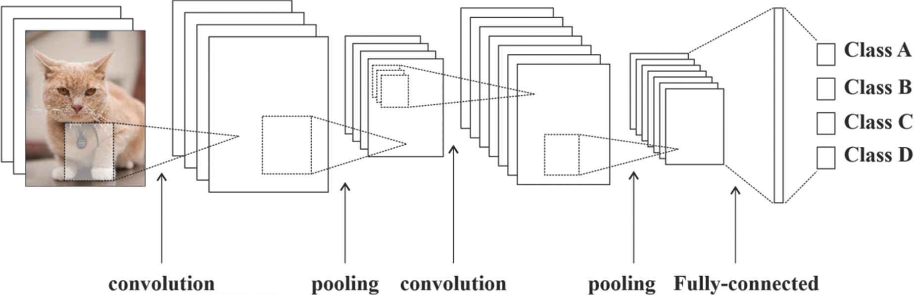
General structure of convolutional neural network.
CNNs produce highly efficient solutions for image recognition problems as deep neural networks. They have surpassed traditional approaches in this respect [26]. However, the design and training of the deep neural networks necessitate a great deal of data and computational resource of very high levels. When the data and resources that are needed to train a deep learning model are considered, pre-trained deep models are highly advantageous compared to deep learning [27].
3.1. AlexNet
AlexNet is the winning evolutionary neural network of the ImageNet large-scale Visual Recognition Competition in 2012 that was held annually [28]. This architecture is pre-trained on the ImageNet database with 1.2 million images of 1000 common objects and has a network structure that is capable of distinguishing 1000 images [29]. It becomes possible to use this network as a feature extractor when the original output layer is identified as a suitable layer for the present classification problem. The pre-trained AlexNet architecture consists basically of five convolutional layers and three fully-connected layers. The structure of the AlexNet model is given in Table 1. The filters that have certain heights and widths in the convolution layer are circulated from the left to the right by strides on the input image. Convolution provides that features are learnt from model images and reduces the complexity of the model. The equation for the convolution process is given in Equation (1). When “R” image is given at (i, j) dimension, the convolution is defined as in Equation (1).
| No. | Layer Name | Layer Type | Description |
|---|---|---|---|
| 1 | ‘data’ | Image Input | 227 × 227 × 3 images with 'zerocenter' normalization |
| 2 | ‘conv1’ | Convolution | 96 11 × 11 × 3 convolutions with stride [4 4], and padding [0 0 0 0] |
| 3 | ‘relu1’ | ReLU | ReLU |
| 4 | ‘norm1’ | Cross Channel Normalization | cross channel normalization with 5 channels per element |
| 5 | ‘pool1’ | Max Pooling | 3 × 3 max pooling with stride [2 2] and padding [0 0 0 0] |
| 6 | ‘conv2’ | Convolution | 256 5 × 5 × 48 convolutions with stride [1 1], and padding [2 2 2 2] |
| 7 | ‘relu2’ | ReLU | ReLU |
| 8 | ‘norm2’ | Cross Channel Normalization | cross channel normalization with 5 channels per element |
| 9 | ‘pool2’ | Max Pooling | 3 × 3 max pooling with stride [2 2] and padding [0 0 0 0] |
| 10 | ‘conv3’ | Convolution | 384 3 × 3 × 256 convolutions with stride [1 1], and padding [1 1 1 1] |
| 11 | ‘relu3’ | ReLU | ReLU |
| 12 | ‘conv4’ | Convolution | 384 3 × 3 × 192 convolutions with stride [1 1], and padding [1 1 1 1] |
| 13 | ‘relu4’ | ReLU | ReLU |
| 14 | ‘conv5’ | Convolution | 256 3 × 3 × 192 convolutions with stride [1 1], and padding [1 1 1 1] |
| 15 | ‘relu5’ | ReLU | ReLU |
| 16 | ‘pool5’ | Max Pooling | 3 × 3 max pooling with stride [2 2] and padding [0 0 0 0] |
| 17 | ‘fc6’ | Fully Connected | 4096 fully connected layer |
| 18 | ‘relu6’ | ReLU | ReLU |
| 19 | ‘drop6’ | Dropout | 50% dropout |
| 20 | ‘fc7’ | Fully Connected | 4096 fully connected layer |
| 21 | ‘relu7’ | ReLU | ReLU |
| 22 | ‘drop7’ | Dropout | 50% dropout |
| 23 | ‘fc8’ | Fully Connected | 1000 fully connected layer |
| 24 | ‘prob’ | Softmax | Softmax |
| 25 | ‘output’ | Classification Output | crossentropyex with ‘tench’ and 999 other classes |
The model of AlexNet in Matlab [30].
The “F” given in the formula refers to the feature map, and the “w” refers to the convolution core along the x, y axis. The input image which consists of 3 color channels at a height of 227-pixel width and at a 227-pixel height is given to the first layer. A 3-channel filter that has a width of 11 pixels and a height of 11 pixels is applied to this input image. A total of 96 filters are applied in the first layer. The next step is the activation function. The Rectified Linear Units are used for activation. This process is applied after each convolution layer. The negative values in the input data are drawn to zero after the end of the convolution. The purpose of ReLU is to bring the deep network into a structure that is not linear. The ReLU function is given in Equation (2).
Similar to the first layer, filters are applied as follows: 256 filters of 5 × 5 in the second layer, 384 filters of 3 × 3 in the third layer, 384 filters of 3 × 3 in the fourth layer; and 256 filters of 3 × 3 in the fifth layer. In addition, pooling is applied after each convolution and ReLU process. The main purpose of the pooling process is feature reduction. It reduces the size of the input image that will be sent to the next convolution layer in terms of width and height; and creates a value that represents neighboring pixel groups in the features map. The maxpooling is shown in Figure 2. The features map is 4 × 4, the maximum pooling feature creates maximum value in each 2 × 2 block and reduces the size of the feature at a significant level.
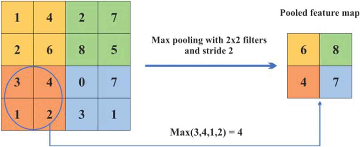
Max pooling.
The last three layers are the fully-connected layers. In the sixth and seventh layers, which are fully-connected, there are 4096 neurons in which all neurons are bound to each other. The last layer is the one where classification is made. After the convolution, ReLU and pooling processes, the fully-connected layer comes. Each neuron in this layer is fully-connected to all neurons of the previous layer.
Each of the FC6 and FC7 layers of AlexNet has 4096 neurons, which are fully-connected to each other. The final layer is the classification layer. The number of the neurons in this layer is the same number of the classes in the dataset. In general, it can be used in different classifiers when Softmax classifier is used. It calculates the probability that any test data belongs to each class. The Softmax Equation is given in (3). Softmax ensures that the neurons have the output values in the range of 0.1.
3.2. VGG-16
The VGG16 pre-trained deep network architecture was developed by Simonyan and Zisserman in the ILSVRC 2014 competition. Basically, it is a deep network that consists of 13 convolution and 3 full-connected layers. It has 41 layers in total including Maxpool, Fullconnected, Relu, Dropout and Softmax layers. The dimension of input layer image is 224 × 224 × 3. The last layer forms the classification layer. Some of the convolution layers are followed by maxpooling for the purpose of reducing dimension. In comparison to AlexNet where bigger filters are used, smaller 3 × 3 filters are used [26]. VGG-16 architecture is shown in Figure 3.
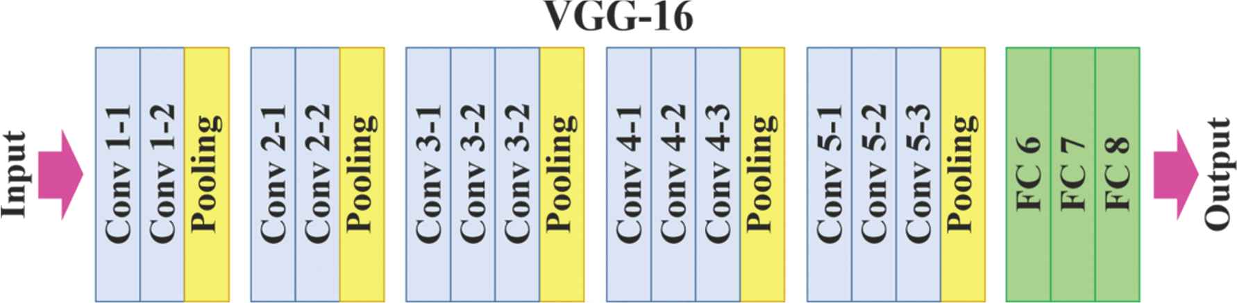
VGG-16 net architecture.
4. THE PROPOSED METHOD
In the present study, a new method for music emotion recognition is proposed by applying the deep learning technique to pre-trained deep networks, which is contrary to the traditional feature-based machine learning methods. The method that is recommended for music emotion recognition consisted of five steps. In the first step, the chroma spectrograms are extracted from the music records in the dataset. In the second step, the dataset increasing process is applied to augment the dataset. For the purpose of augmentation the data, two different deformations are applied to each music recording in the dataset to make it six times bigger. In the third step, the chroma spectrograms are given as inputs to the AlexNet model, which is pre-trained with one million images. The proposed method is built on AlexNet but the same tests were also made with the aid of VGG-16 for observing the efficiency of pre-trained deep networks in music emotion recognition. In the fourth step, the deep feature extraction layers are determined. In the fifth step, the classification process is performed by using the deep visual features that are extracted.
The layer following Fc8 layer in AlexNet and VGG-16 models is the classifying layer, and Softmax is the internal classifier. In this study, both SVM and Softmax are used as classifier subsequently to Fc8. These classifiers are trained by using the SVM with linear kernel and Softmax as the classifiers with training and test data that are obtained at different rates. The working principle of the proposed method is as given in Figure 4.
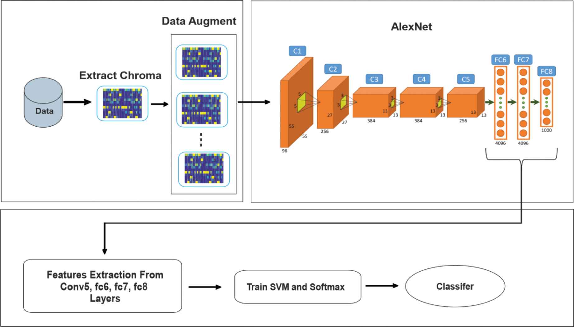
Working principle of the proposed.
4.1. Extracting Chroma Spectrograms
The chroma shows the energy distribution around each note. Each note has a certain frequency range. It calculates the energy density in these frequency ranges of the relevant notes. Chroma spectrograms are extracted in experimental studies by using the MIRtoolbox [31]. A sample sound signal and the chroma image are given in Figure 5. There are seven notes; and since the interval between two sounds is divided into two equal parts except for notes E and F, 12 features and the chroma spectrogram can be obtained by including the sound in between.
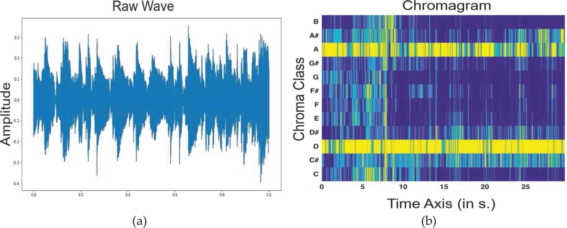
Illustration of sound signal and chroma spectrogram (a) sound signal, (b) chroma spectrogram.
4.2. Data Augmentation
In deep learning, a large amount of training data is needed in many times to have satisfactory classification performance rates and to reduce the error gap between the training data and the test data [32]. When the size of the original data is limited, it is necessary to augment the data to overcome this drawback. Data augmentation means the creation of additional training data samples by applying a series of deformation data to the ones in the training dataset [33]. The basic principle in data augmentation process is that the labels of the new data do not change with the help of the deformations that are applied to the labeled data [34]. There are many techniques for data augmentation like rotating the image at different angles, horizontal–vertical rotation, and adding noise and color manipulations to the image. In this study, before the chroma spectrogram of each sample is extracted in the dataset, two different operations are applied to the signal. The first is shifting, and the second one is stretching. The sound samples that are obtained at the end of each process are added to the original sound sample class as new data.
Time Stretch: We are willing to increase or decrease the speed of the audio samples while pitches remain the same. Each sample was time stretched by four factors, respectively, 0.81, 0.93, 1.07, 1.23.
Time Shifting: The sound is shifted from the starting point and the original length is maintained. Each instance was shifted from the starting point to 5 seconds.
When the original sample in the dataset was also included, the size of our dataset became six-fold. The notation of the audio signals before and after data augmentation and the chroma features are given in Figure 6. In Algorithm 1, the pseudo code of the data augmentation algorithm is given.
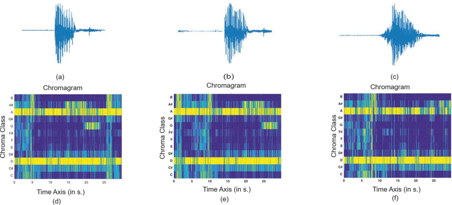
Illustration of data augmentation (a) original signal, (b) shifting signal, (c) stretch signal, (d) original chroma, (e) shifting chroma, (f) stretch chroma.
Algorithm 1: Data Augmentation Algorithm
Input: sf : Sound File
sr : Sample rate
ns: Number of stretching
tst1, ts2, ts3, ts4: Four different time stretching.
tsh : Time shifting rate (second).
Algorithm:
1: Initialize and assign input parameters (sf, sr, tst1, tst2, tst3, tst4, tsh)
2: data = Read Audio File(sf.Name)
3: shifting sound = Time shifting(data, sr * tsh)
4: for i:= 1 to ns do
5: input_length = len(data)
6: stretching_ sound(i) = stretch(data, tst(i))
7: if len(stretching_ sound(i)) > input_length then
8: Stretching_ sound(i) = data[:input_length]
9: end if
10: end for
11: Write audio file (‘folder name/’+Filename+'_ shifting sound.mp3’, shifting sound, sr)
12: Write audio file (‘foldername/’+Filename+'_ stretching_ sound1.mp3’, stretching_ sound (1), sr
13: Write audio file (‘foldername/’+Filename+'_ stretching_ sound2.mp3’, stretching_ sound (2), sr)
14: Write audio file (‘foldername/’+Filename+'_ stretching_ sound3.mp3’, stretching_ sound (3), sr)
15: Write audio file (‘foldername/’+Filename+'_ stretching_ sound4.mp3’, stretching_ sound (4), sr)
4.3. Deep Feature Extraction Process
In this study, pre-trained deep network models, which means the application of deep learning, was used to classify the new object class; and in this respect, the AlexNet and VGG-16 model are examined. When we want to classify our own datasets with these pre-trained architectures, the deep learning process can be applied on different models. We may re-train these networks with our own dataset by changing some layers at the end of the pre-trained networks, or we may train a classifier by extracting some deep features from our own dataset and by using these networks.
In the present study, the deep learning process is carried out by extracting deep features from the layers of the AlexNet and VGG-16 and then, some of these deep feature records are used to train the classifiers and some of them is used to test the classifiers. Basically, the AlexNet and VGG-16 has convolutions and fully-connected layers, which can be employed as feature extractor layers. The conv5, Fc6, Fc7 and Fc8 layers of the AlexNet and conv5_3, Fc6, Fc7 and Fc8 layers of theVGG-16 are chosen as the feature-extractor layers in this study. The AlexNet and VGG-16 model that are in the MATLAB software is employed for the application.
5. EXPERIMENTAL APPLICATIONS
5.1. Datasets
To evaluate the performance of music emotion classification, we use the Soundtracks [35–37] dataset and our newly prepared dataset. Soundtracks involve six categorical mood classes, that consist of happiness, sadness, fear, anger, surprise and tenderness. All of the 30 music clips included in each of the classes in the Sountracks dataset last 18–30 seconds of duration. When the studies in this field were examined, it was determined that most researchers prepared their own datasets instead of using a common one because it is still not possible to claim that there is a common dataset in this field. There is still no consensus on which emotion models should be used or how many emotion categories should be considered [38]. Aside from this, the subjective nature of human perception makes the creation of a common database difficult. For these reasons, we prepared our own dataset for this study. To prepare the dataset, verbal and non-verbal music are selected from different genres of Turkish music. The dataset is designed as a discrete model, and there are four classes in the dataset: happy, sad, angry, relax. The participants are asked to label the selected music with “happy,” “sad,” “angry,” “relax” emotion labels in the experiment in which 13 people participated to determine the emotions of these music pieces. Thirty-second parts of the selected music pieces are randomly played to the participants, who are asked to label the music according to their feelings. Then, according to these labels, the emotion classes of the music pieces were determined. The label that is most used by the participants is included in that class. If the label is tagged with music, the label was included in the class. For example, if a music piece is labeled as “relax” by 10 participants, and as “happy” by 3 participants, it was included in the “relax” class. The experiment is conducted in 3 sessions, and each participant listened to 500 music in total. A total of 100 music pieces are determined for each class in the database to have an equal number of samples in each class. The remaining music pieces are not taken into consideration. There are 400 samples in the original dataset as 30 seconds from each sample.
In addition, two datasets are made into six-fold after data augmentation. The Soundtracks dataset, the our dataset and the number of records that are obtained after data augmentation are given in Tables 2 and 3, respectively. As far as we are concerned, music emotion recognition has not been carried out by using the data in Turkish music so far. The dataset is shared here for the researchers who would like to study in this field.
| Class | Number of Data Before Augmentation | Number of Data After Augmentation |
|---|---|---|
| Anger | 30 | 180 |
| Fear | 30 | 180 |
| Happy | 30 | 180 |
| Sad | 30 | 180 |
| Surprise | 30 | 180 |
| Tender | 30 | 180 |
Soundtracks dataset—number of data in each class before and after data augmentation.
| Class | Number of Data Before Augmentation | Number of Data After Augmentation |
|---|---|---|
| Happy | 100 | 600 |
| Sad | 100 | 600 |
| Angry | 100 | 600 |
| Relax | 100 | 600 |
Our dataset—number of data in each class before and after data augmentation.
(The link: https://drive.google.com/open?id=1TfHtRoX73yIJd40QNLEhYzgH_wlhQSLz)
5.2. Settings
The application of the proposed method is applied in a computer that had i7 2.50GHz processor, 12GB memory and NVIDIA 940M GPU. The software codes required for the application are prepared by using the MATLAB software matlab2018a version. Python programming language is used for data augmentation.
5.3. Statistical Evaluation of Performance
In this study, statistical testing is employed to confirm the results obtained by the proposed method. Wilcoxon Rank Sum test is used for evaluation. The Wilcoxon test is a non-parametric statistical test comparing two paired groups. The test essentially calculates the difference between each pair of data and analyzes these differences [39]. “P” value is calculated at the end of the test. “P” value is used to determine whether the relationship or difference between the data pairs is statistically significant or not. It also identifies the level of existing relationship and difference. Any “P” value below 0.05 indicates a significant difference.
5.4. Experimental Results
For the purpose of calculating the classification accuracy, experiments were done by using the augmented dataset and the original one with deep features that were extracted from different the AlexNet and VGG-16 layers. Some of the data that are collected from the dataset randomly are used for training, and the remaining part is used for the test. For the purpose of determining the effect of the size of the data that were spared for training and testing on the performance of the network, these data are divided in three different ways. In the first experiment, 50% of the data are used for training and 50% are used for testing; in the second experiment, 60% of the data are used for training and 40% are used for testing; and in the third experiment, 70% of the data are used for the training and 30% are used for testing.
The classification results of the Softmax and SVM on our dataset that are trained with the features that are obtained from various layers of the AlexNet like “Conv5,” “Fc6,” “Fc7” and “Fc8” are given in Tables 4–7, respectively. In addition, the classification results for all layers of the AlexNet on the soundtracks dataset are given in Table 8.
| Layer | Classifier | Training–Testing Data Splitting | Accuracy Before Augmentation (%) | Accuracy After Augmentation (%) |
|---|---|---|---|---|
| Conv5 | SVM | 50%–50% | 53.5 | 61.1 |
| Conv5 | SVM | 60%–40% | 56.9 | 63.6 |
| Conv5 | SVM | 70%–30% | 58.3 | 64.0 |
| Conv5 | Softmax | 50%–50% | 53.5 | 62.3 |
| Conv5 | Softmax | 60%–40% | 54.4 | 62.4 |
| Conv5 | Softmax | 70%–30% | 57.5 | 66.3 |
The classification results for Conv5 layer of the AlexNet on our dataset.
| Layer | Classifier | Training–Testing Data Splitting | Accuracy Before Augmentation (%) | Accuracy After Augmentation (%) |
|---|---|---|---|---|
| Fc6 | SVM | 50%–50% | 69.5 | 85.7 |
| Fc6 | SVM | 60%–40% | 73.1 | 87.0 |
| Fc6 | SVM | 70%–30% | 74.0 | 87.4 |
| Fc6 | Softmax | 50%–50% | 67.5 | 83.1 |
| Fc6 | Softmax | 60%–40% | 71.3 | 85.3 |
| Fc6 | Softmax | 70%–30% | 74.2 | 85.6 |
The classification results for the Fc6 layer of the AlexNet on our dataset.
| Layer | Classifier | Training–Testing Data Splitting | Accuracy Before Augmentation (%) | Accuracy After Augmentation (%) |
|---|---|---|---|---|
| Fc7 | SVM | 50%–50% | 70.0 | 84.0 |
| Fc7 | SVM | 60%–40% | 71.3 | 85.8 |
| Fc7 | SVM | 70%–30% | 72.5 | 88.5 |
| Fc7 | Softmax | 50%–50% | 69.0 | 79.6 |
| Fc7 | Softmax | 60%–40% | 70.6 | 83.4 |
| Fc7 | Softmax | 70%–30% | 73.3 | 85.3 |
Classification results for Fc7 layer of the AlexNet on our dataset.
| Layer | Classifier | Training–Testing Data Splitting | Accuracy Before Augmentation (%) | Accuracy After Augmentation (%) |
|---|---|---|---|---|
| Fc8 | SVM | 50%–50% | 63.5 | 80.8 |
| Fc8 | SVM | 60%–40% | 63.7 | 82.3 |
| Fc8 | SVM | 70%–30% | 68.8 | 84.0 |
| Fc8 | Softmax | 50%–50% | 63.1 | 77.2 |
| Fc8 | Softmax | 60%–40% | 66.9 | 79.1 |
| Fc8 | Softmax | 70%–30% | 70.8 | 81.0 |
Classification results for Fc8 layer of the AlexNet on our dataset.
| Layer | Classifier | Training–Testing Data Splitting | Accuracy Before Augmentation (%) | Accuracy After Augmentation (%) |
|---|---|---|---|---|
| Conv5 | SVM | 50%–50% | 25.0 | 45.0 |
| Conv5 | SVM | 60%–40% | 25.6 | 46.3 |
| Conv5 | SVM | 70%–30% | 31.5 | 49.7 |
| Conv5 | Softmax | 50%–50% | 25.0 | 40.4 |
| Conv5 | Softmax | 60%–40% | 27.8 | 42.6 |
| Conv5 | Softmax | 70%–30% | 30.6 | 43.5 |
| Fc6 | SVM | 50%–50% | 32.2 | 71.5 |
| Fc6 | SVM | 60%–40% | 40.3 | 73.8 |
| Fc6 | SVM | 70%–30% | 40.7 | 74.4 |
| Fc6 | Softmax | 50%–50% | 36.7 | 69.6 |
| Fc6 | Softmax | 60%–40% | 38.8 | 71.1 |
| Fc6 | Softmax | 70%–30% | 46.3 | 72.5 |
| Fc7 | SVM | 50%–50% | 30.0 | 65.7 |
| Fc7 | SVM | 60%–40% | 36.1 | 69.2 |
| Fc7 | SVM | 70%–30% | 38.9 | 72.2 |
| Fc7 | Softmax | 50%–50% | 27.8 | 63.5 |
| Fc7 | Softmax | 60%–40% | 37.5 | 67.1 |
| Fc7 | Softmax | 70%–30% | 40.7 | 70.4 |
| Fc8 | SVM | 50%–50% | 31.1 | 61.3 |
| Fc8 | SVM | 60%–40% | 31.9 | 64.1 |
| Fc8 | SVM | 70%–30% | 33.3 | 67.9 |
| Fc8 | Softmax | 50%–50% | 30.0 | 59.8 |
| Fc8 | Softmax | 60%–40% | 36.1 | 60.6 |
| Fc8 | Softmax | 70%–30% | 38.9 | 66.0 |
The classification results for each layers of the AlexNet on soundtracks dataset.
The classification results of the “Conv5” layer of the AlexNet are given in Table 4. As seen in the data in Table 4, the highest classification success was obtained as 58.3% with SVM before the data augmentation process. Following the data augmentation, the highest classification success was obtained as 66.3% with Softmax. The Confusion matrixes of the best classification results of “Conv5” layer before and after data augmentation are given in Figure 7.
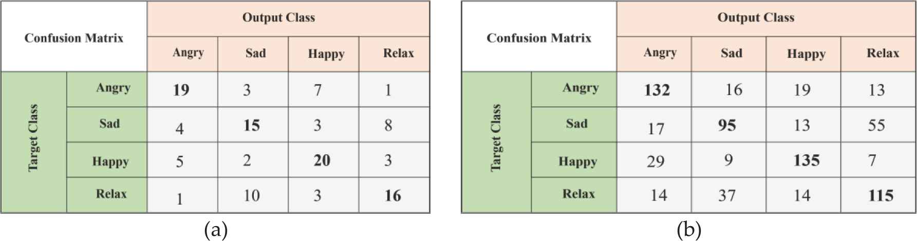
Conv5 layer—Confusion matrix (a) Confusion matrix before data augmentation, (b) Confusion matrix after data augmentation.
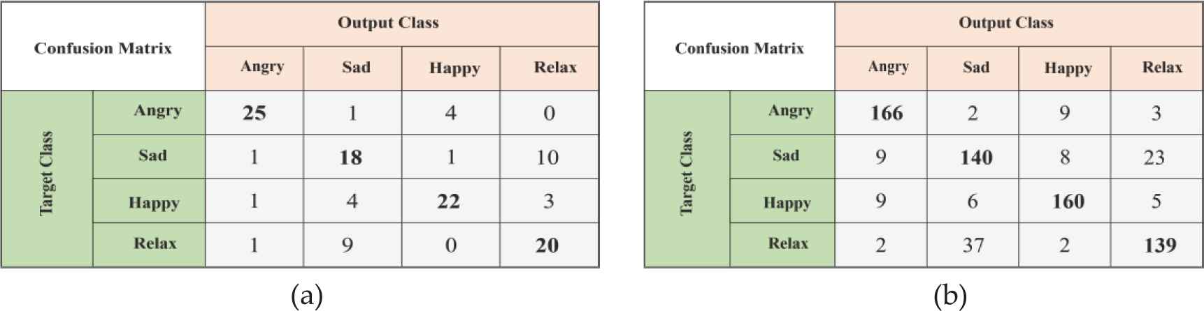
The classification results of the “Fc6” layer of the AlexNet are given in Table 5. As seen in Table 5, the highest classification success as a result of the division of the dataset for training and testing before data augment (70%–30%, respectively) was 74.2% with Softmax. After data augmentation, the highest classification success was obtained with SVM as 87.4% by dividing the dataset for training and testing (70%–30%, respectively). The Confusion matrices of the best classification results before and after data augmentation are given in Figure 8 for “Fc6” layer.
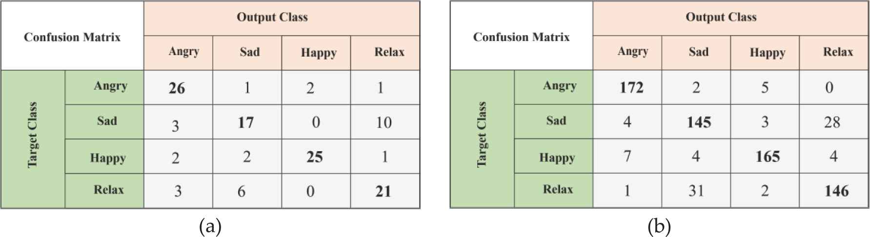
Fc6 layer—Confusion Matrix (a) Confusion matrix before data augmentation, (b) Confusion matrix after data augmentation.
The classification results for the “Fc7” layer of the AlexNet are given in Table 6. As seen in the data in Table 6, the highest classification success was obtained with Softmax at a rate of 73.3% by dividing the dataset for training and testing (70%–30%, respectively) before data augmentation. After the data augmentation, the highest classification success was obtained with SVM by dividing the dataset for training and testing (70%–30%, respectively) with SVM as 88.5%. The Confusion matrices of the best classification results before and after data augmentation are given in Figure 9 for “Fc7” layer.
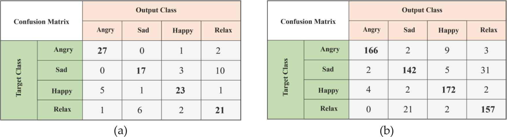
Fc7 layer—Confusion matrix (a) Confusion matrix before data augmentation, (b) Confusion matrix after data augmentation.
The classification results for the “Fc8” layer of the AlexNet are given in Table 7. As seen in the data in Table 7, the highest classification success was obtained with Softmax at a rate of 70.8% by dividing the dataset for training and testing (70%–30%, respectively) before data augmentation. The highest classification success was obtained with SVM by dividing the dataset for training and testing (70%–30%, respectively) after the data augmentation with 84.0%. The Confusion matrices of the best classification results before and after data augmentation are given in Figure 10 for “Fc8” layer.
Fc8 layer—Confusion matrix (a) Confusion matrix before data augmentation, (b) Confusion matrix after data augmentation.
The classification results obtained from each layer of AlexNet with the soundtrack data set are given in Table 8. The highest classification success was obtained from Fc6 layer with Softmax at a rate of 46.3% by dividing the dataset for training and testing (70%–30%, respectively) before data augmentation. The highest classification success was obtained from Fc6 layer with SVM by dividing the dataset for training and testing (70%–30%, respectively) after the data augmentation with 74.4%.
The classification results for all layers of VGG-16 on the our dataset and soundtracks dataset are given in Tables 9 and 10, respectively. According to the results in Table 9, the highest classification success was obtained from Fc6 layer with Softmax at a rate of 76.0% by dividing the dataset for training and testing (70%–30%, respectively) before data augmentation. The highest classification success was obtained from Fc6 layer with Softmax by dividing the dataset for training and testing (70%–30%, respectively) after the data augmentation with 89.2%.
| Layer | Classifier | Training–Testing Data Splitting | Accuracy Before Augmentation (%) | Accuracy After Augmentation (%) |
|---|---|---|---|---|
| Conv5_3 | SVM | 50%–50% | 54.8 | 61.3 |
| Conv5_3 | SVM | 60%–40% | 58.2 | 62.8 |
| Conv5_3 | SVM | 70%–30% | 61.6 | 66.1 |
| Conv5_3 | Softmax | 50%–50% | 55.7 | 64.3 |
| Conv5_3 | Softmax | 60%–40% | 55.9 | 65.2 |
| Conv5_3 | Softmax | 70%–30% | 58.3 | 69.0 |
| Fc6 | SVM | 50%–50% | 72.3 | 83.5 |
| Fc6 | SVM | 60%–40% | 74.7 | 87.2 |
| Fc6 | SVM | 70%–30% | 78.6 | 88.0 |
| Fc6 | Softmax | 50%–50% | 70.0 | 81.4 |
| Fc6 | Softmax | 60%–40% | 71.8 | 85.8 |
| Fc6 | Softmax | 70%–30% | 76.0 | 86.7 |
| Fc7 | SVM | 50%–50% | 69.0 | 83.1 |
| Fc7 | SVM | 60%–40% | 69.4 | 86.0 |
| Fc7 | SVM | 70%–30% | 73.2 | 89.2 |
| Fc7 | Softmax | 50%–50% | 68.0 | 80.7 |
| Fc7 | Softmax | 60%–40% | 70.0 | 81.4 |
| Fc7 | Softmax | 70%–30% | 73.3 | 83.2 |
| Fc8 | SVM | 50%–50% | 64.0 | 82.4 |
| Fc8 | SVM | 60%–40% | 67.5 | 84.6 |
| Fc8 | SVM | 70%–30% | 70.0 | 85.0 |
| Fc8 | Softmax | 50%–50% | 65.5 | 79.2 |
| Fc8 | Softmax | 60%–40% | 67.5 | 79.6 |
| Fc8 | Softmax | 70%–30% | 72.5 | 81.4 |
The classification results for each layers of the VGG-16 on our dataset.
| Layer | Classifier | Training–Testing Data Splitting | Accuracy Before Augmentation (%) | Accuracy After Augmentation (%) |
|---|---|---|---|---|
| Conv5_3 | SVM | 50%–50% | 24.2 | 47.8 |
| Conv5_3 | SVM | 60%–40% | 25.8 | 49.4 |
| Conv5_3 | SVM | 70%–30% | 30.4 | 50.2 |
| Conv5_3 | Softmax | 50%–50% | 25.0 | 42.5 |
| Conv5_3 | Softmax | 60%–40% | 29.3 | 43.8 |
| Conv5_3 | Softmax | 70%–30% | 32.0 | 47.6 |
| Fc6 | SVM | 50%–50% | 30.2 | 72.4 |
| Fc6 | SVM | 60%–40% | 37.6 | 74.7 |
| Fc6 | SVM | 70%–30% | 38.9 | 75.5 |
| Fc6 | Softmax | 50%–50% | 33.3 | 71.3 |
| Fc6 | Softmax | 60%–40% | 37.7 | 72.5 |
| Fc6 | Softmax | 70%–30% | 42.5 | 73.8 |
| Fc7 | SVM | 50%–50% | 30.0 | 67.3 |
| Fc7 | SVM | 60%–40% | 37.5 | 70.8 |
| Fc7 | SVM | 70%–30% | 40.8 | 71.2 |
| Fc7 | Softmax | 50%–50% | 31.3 | 65.0 |
| Fc7 | Softmax | 60%–40% | 36.7 | 68.4 |
| Fc7 | Softmax | 70%–30% | 39.0 | 72.7 |
| Fc8 | SVM | 50%–50% | 34.2 | 62.3 |
| Fc8 | SVM | 60%–40% | 35.7 | 66.7 |
| Fc8 | SVM | 70%–30% | 37.0 | 68.2 |
| Fc8 | Softmax | 50%–50% | 30.8 | 61.2 |
| Fc8 | Softmax | 60%–40% | 34.6 | 63.4 |
| Fc8 | Softmax | 70%–30% | 40.2 | 68.1 |
The classification results for each layers of the VGG-16 on soundtracks dataset.
According to the results in Table 10, the highest classification success was obtained from Fc6 layer with Softmax at a rate of 42.5% by dividing the dataset for training and testing (70%–30%, respectively) before data augmentation. The highest classification success was obtained from Fc6 layer with SVM by dividing the dataset for training and testing (70%–30%, respectively) after the data augmentation with 75.5%.
In order to evaluate the performance of the proposed method better, the Soundtracks dataset, that is used in the context music information retrieval, is tested with the proposed method, and results are compared with the results gained from other methods used in the literature. Both results acquired from different methods and the proposed method are shown in Table 11.
| Approach | Accuracy |
|---|---|
| Ren et al. [18] | 43.56 |
| Panagakis and Kotropoulos [36] | 39.44 |
| Mo and Niu [37] | 44.68 |
| Proposed System (Before Data Augmentation) | 46.3 |
| Proposed System (After Data Augmentation) | 75.5 |
Performance comparison with other approaches on the soundtracks dataset.
It is clear from the Table 11 that the proposed method, in which data augmentation is applied, has a way better performance than those of other three methods used in the literature. In light of this evidence, it is seen that the proposed architecture can be used effectively for the task of recognizing emotions in music.
Moreover, the Wilcoxon Rank Sum test is administered for experimental results obtained by different methods and these results are given in Table 12. According to Wilcoxon Rank Sum test, “P” < 0.05 is required for a meaningful relationship between the results obtained by different methods. As can be seen in the data in Table 12, “P” value is generally close to zero as a result of the comparison of diverse methods. In this case, it shows us that there is a significant relationship between the results.
| Compared Results | P Value for Our Data Set | P Value for Soundtracks Data Set |
|---|---|---|
| AlexNet + Before Augmentation & AlexNet + After Augmentation |
≈ 0 | ≈ 0 |
| VGG-16 + Before Augmentation & VGG-16 + After Augmentation |
≈ 0 | ≈ 0 |
| AlexNet & VGG-16 (Before Augmentation) |
0.002 | 0.909 |
| AlexNet & VGG-16 (After Augmentation) |
0.141 | ≈ 0 |
Wilcoxon rank sum test results.
6. CONCLUSION
In this study, a new method for music emotion recognition that used pre-trained deep network, which is the application of deep learning models, is presented. Deep learning technique is applied to a pre-trained network by using data augmented the chroma spectrograms that are obtained from musical data, and the classification success rate of music emotion recognition is increased by using deep visual features that are extracted from the chroma spectrograms. For this purpose, the pre-trained network model, AlexNet architecture and VGG-16, are used. With the dataset that is prepared for this study and soundtracks dataset, deep visual features are extracted from different layers of the AlexNet and VGG-16. These deep visual features are used to train and test SVM and Softmax classifiers. The best classification success before data augmentation is obtained from the “Fc6” layer of the VGG-16 with Softmax classifier with 76% on our dataset. After the data augmentation, the best classifier success was obtained from the “Fc7” layer of the VGG-16 with the SVM classifier with 89.2% on our dataset. The accuracy rate increased after the data augmentation, which is an expected situation. According to the results, it is determined that pre-trained deep learning model can be used for music emotion recognition problem; and in addition, it is also determined that pre-trained deep neural networks are very effective method even if the original training data is limited. It is recommended for future studies that these networks are pre-trained with existing datasets, and music emotion recognition is investigated by using different pre-trained deep network architecture models.
CONFLICT OF INTEREST
Authors have no conflict of interest to declare.
Funding Statement
There is no funding for this project.
AUTHORS' CONTRIBUTIONS
Author contributions are equal and same 50%.
REFERENCES
Cite this article
TY  - JOUR
AU  - Mehmet Bilal Er
AU  - Ibrahim Berkan Aydilek
PY  - 2019
DA  - 2019/12/20
TI  - Music Emotion Recognition by Using Chroma Spectrogram and Deep Visual Features
JO  - International Journal of Computational Intelligence Systems
SP  - 1622
EP  - 1634
VL  - 12
IS  - 2
SN  - 1875-6883
UR  - https://doi.org/10.2991/ijcis.d.191216.001
DO  - 10.2991/ijcis.d.191216.001
ID  - BilalEr2019
ER  -