
A Statistical Approach to Provide Explainable Convolutional Neural Network Parameter Optimization
- DOI
- 10.2991/ijcis.d.191219.001How to use a DOI?
- Keywords
- Optimization; Convolutional neural network; Hyperparameter; Design of experiment; Taguchi; Deep learning
- Abstract
Algorithms based on convolutional neural networks (CNNs) have been great attention in image processing due to their ability to find patterns and recognize objects in a wide range of scientific and industrial applications. Finding the best network and optimizing its hyperparameters for a specific application are central challenges for CNNs. Most state-of-the-art CNNs are manually designed, while techniques for automatically finding the best architecture and hyperparameters are computationally intensive, and hence, there is a need to severely limit their search space. This paper proposes a fast statistical method for CNN parameter optimization, which can be applied in many CNN applications and provides more explainable results. The authors specifically applied Taguchi based experimental designs for network optimization in a basic network, a simplified Inception network and a simplified Resnet network, and conducted a comparison analysis to assess their respective performance and then to select the hyperparameters and networks that facilitate faster training and provide better accuracy. The results show that up to a 6% increase in classification accuracy can be achieved after parameter optimization.
- Copyright
- © 2019 The Authors. Published by Atlantis Press SARL.
- Open Access
- This is an open access article distributed under the CC BY-NC 4.0 license (http://creativecommons.org/licenses/by-nc/4.0/).
1. INTRODUCTION
Convolutional neural networks (CNNs) have been widely used for image recognition [1], including hyperspectral data classification [2] and video classification [3]. Reducing the architecture size of CNNs, in term of their particular task and dataset, makes them more attractive for use in mobile phones and embedded systems, where less power consumption and overall cost reduction are crucial factors [4–8]. To date, designing state-of-the-art CNN algorithms for specific datasets, such as images, has been time-consuming (manually engineered) and computationally intensive [8–13]. Some techniques have been proposed for automatically designing CNNs, however, these techniques either require huge computational resources or do not match manually-engineered accuracies [14–18]. In addition, for many applications, the complexity of automatically designed CNN algorithms render them neither interpretable nor explainable enough to be used safely [19,20]. Using a statistical approach to optimize the performance of CNN models not only helps build optimum networks according to required criteria, but also makes models more explainable. Statistical experimental designs have been widely applied to various optimization problems [21–23] including parameter optimization of perceptron neural networks [24–26]. However, for proper optimization of the hyperparameters of deep learning networks, the design of experiment (DOE) is powerful technique, and, to our knowledge, this has never been investigated. In this paper, we propose DOE algorithms based on applying Taguchi statistical methods [27] for optimizing CNN parameters, whereby spectral agricultural data is evaluated using three simplified CNN architectures. Finally, to validate our new approach the results are compared with award-winning CNN architectures.
2. EXPERIMENTAL METHODS
The proposed primitive cells that are the building blocks of the proposed CNN network, are described and compared with those used in current state-of-the-art conventional CNN network architectures. Next, the Taguchi method is introduced with four experiments conducted to optimize the various parameters of the CNN network.
2.1. The Convolutional Neural Network Primitives
Most CNNs require huge memory and computational resources. Therefore, the size of the CNN becomes important for applications running on limited resources (e.g., limited speed and memory of mobile phones). In this study, in order to build up an efficient CNN network, primitive blocks from well-known CNN architectures have been adapted and used, namely, the VGG network, the Inception network, and the Resnet network [10,11,13].
2.1.1. Simple primitive block
The simple primitive block of the proposed CNN was designed to include a convolutional layer with batch normalization, Rectified Linear Unit (ReLu) function, and max pooling. The advantage of using ReLu instead of traditional neural network functions, like sigmoid or hyperbolic functions, is that training is typically faster. The ReLu formula is f(x) = max (0, x) [27]. The batch normalization, which is normalization of the network's weights in each layer, has many advantages, including faster learning rate convergence, efficient weight initialization, and additional regularization, all of which result in faster training with lower overfitting [28]. Max pooling reduces the computation by extracting the most important features from a kernel, thereby producing a smaller feature representation [29,30].
2.1.2. The Inception primitive blocks
The Inception network is based on the concept that many activations in deep convolution layers are either excessive (zero value) or redundant (highly correlated). Therefore, instead of going deeper in the CNN network, the balance between network width and depth should be maintained in order to provide optimal performance. The necessity of having efficient dimension reduction leads to a sparse network with various filter sizes. As a result, the required computational reduction leads to bottleneck convolution [31] Szegedy, Vanhoucke [13] have suggested that replacing
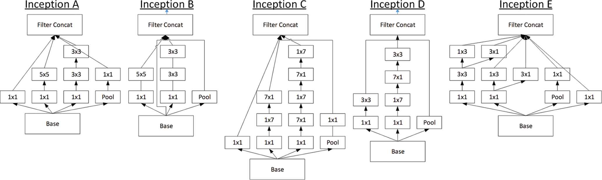
Five asymmetric configurations used Inception blocks for primitive blocks.
2.1.3. The Resnet primitive blocks
The Resnet network was designed to address the challenge of overcoming the vanishing gradient problem in order to build deeper CNNs [11]. Instead of simply stacking layers, the middle layer learns the residual mapping of the input. This is done by adding a residual block as the identity connection from previous layers, thus allowing the residual mapping to be trained [11] as illustrated in Figure 2.

Illustration of a residual block where the middle layer learns the residual mapping of the input, thus allowing the residual mapping to be trained [11].
2.2. Taguchi Method
The Taguchi method is a statistically robust technique, proposed by Geninchi Taguchi [32], which fulfils two main roles, namely, finding factors that provide more variation in responses and finding the best levels of these factors that optimize CNN response. In the Taguchi method, initially a decision is made on which factors can be effective for the required response. Then, the levels of those factors are set. In Figure 3, the Taguchi process block diagram is shown, where the initial process of finding the effective factors is depicted as the preparation block.

The process of implementation of Taguchi design.
The next step in the Taguchi procedure is designing the experiment. This is based on the orthogonal matrix, determining in each run the levels of the control factors that must be taken. In statistical experimental design, orthogonality involves providing a matrix of runs that have statistically independent factors in their columns, where the levels in the columns of the independent factors are orthogonal to one another. Consequently, if the factor levels are considered as a vector, the inner product of mutual factor vectors in an orthogonal array must be zero [33].
Another property of the orthogonal matrix is that all the levels in each column must appear the same number of times. The above-mentioned two properties effectively reduce the number of experiments from full factorial design into a minimal number of runs, which still can provide enough knowledge in describing the effect of factors on the CNN performance. The minimum number of experiments needed to conduct the Taguchi method can be calculated based on the following equation:
The orthogonal matrices in a standard Taguchi design are predefined based on the number of controlling factors and levels. Consequently, the experiment is run according to the defined orthogonal array in order to determine and prepare the CNN responses for analysis. This step is shown as “design a new experiment” in Figure 3. The relative percentage difference (RPD) in accuracy was used as the CNN response indicator that enables better understanding of the impact of the factors on the performance of the CNN architecture. For the generated results, the RPD was calculated as follows:
The results were analysed by comparing the mean controlling factors and signal-to-noise ratios, as well as evaluating the analysis of variance (ANOVA), in order to investigate the significant factors. The preliminary design of the experiment was slightly changed after analysing the results mainly to determine the best controlling factor or the best levels of the controlling factors. After obtaining acceptable RPD results, the optimum level of each factor was implemented to obtain the best CNN according to defined objectives.
2.3. Design of Experiment
Before determining the factors and levels for designing the CNNs, a few preliminary designs were run to evaluate some hyperparameters. Two controlling factors, namely batch size with level values 8, 16, 32, and number of epochs with level values 5, 10, 20, were examined. It was found that neither the batch size nor the number of epochs affected the RPD accuracy. Their p-values in the ANOVA were 0.23 and 0.71, respectively. However, it was necessary to define their values in the network. As the larger batch size resulted in faster training and less over fitting, the selected batch size value was 32. Smaller values for the number of epochs typically led to faster running of the whole procedure of learning. Therefore, the chosen number of epochs was 5.
The following hyperparameters were selected as the factors in our search space: learning rate, augmentation types, number of filters, and size of kernel.
Learning rate: In order to have fast network convergence during training, the optimum selection of the learning rate was essential. When the chosen learning rate was too small, training took too long to converge or the optimizer became trapped in local minima, hence the loss function could not be updated to generalize the network. When the chosen learning rate was too large, the network did not always converge as it might have overpassed the minimum loss function, and hence, made the loss function worse.
Augmentation: Large data in deep learning normally yields better performance; however, it is not always possible to have large data. As neural networks have invariance characteristics, data augmentation can generate more data without the need for additional data collection. In order to select the type of data augmentation, it is necessary to consider the nature of the data. In the proposed study, the implemented data was linear spectrum reflectance. According to the nature of the data, flipping (horizontal and vertical) and normalization were the most suitable transformations for data augmentation.
Number of filters and kernel sizes: In the first two layers of the first design, two simple primitive blocks were used. In the first layer, lower levels for the number of filters were used (4, 8, 16, 32), since the network typically extracts basic features in this layer. The larger levels for the number of filters were selected in the second layer (32, 64, 128, 256), because this layer combines the basic features and produces more complex features for classification. The next factors investigated in the proposed study were the kernel sizes. The levels of 3 and 5 were selected for the investigation.
Four experiments were designed, based on (i) simplified primitive cells, (ii) modified Inception cells, (iii) modified Resnet cells, and (iv) an experiment comparing the performances of all three primitive cells. The pytorch deep learning library [34] was used for all trainings. GeForce GTX 1080Ti Nvidia GPU was the hardware platform for data processing, which has a 11 GB memory, a 352-bit interface used in conjunction with an Intel
2.3.1. First design of experiment
Two simple structures were suggested for the first design, as shown in Figure 4. The first structure had one fully connected classification output layer with soft max activation. The second structure had an extra fully connected layer with a ReLu activation.

Two different convolutional neural networks (CNN) structures comprising simple primitive blocks.
The effect plot and accuracy versus the size of the middle connected layer, which are the results of the preliminary experiment that was designed to choose the number of nodes in the extra fully connected layer, are shown in Figure 5.
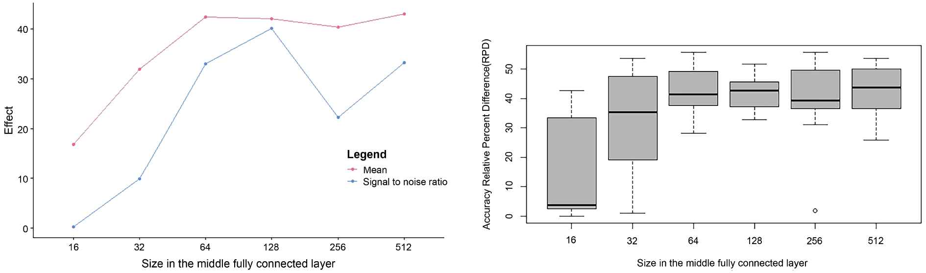
Preliminary experiment results for determining the value of middle fully connected layer in the first design. A) Effect and B) accuracy versus the size of the middle connected layer.
According to the Bonferroni post-hoc test, which measures the significance of the pairwise differences between factor levels, there was no significant difference between the levels with values of 32, 64, 128, and 256 (Table 1). Therefore the 128 value was selected based on the best signal-to-noise-ratio performance. With this result, the first DOE was designed as illustrated in Table 2.
| Df | Sum Sq | Mean Sq | F value | Pr( |
|
|---|---|---|---|---|---|
| Fully connected size | 1 | 2388.6 | 2388.6 | 10.803 | 0.001457** |
| Residuals | 88 | 19457.7 | 221.11 |
Signif. codes: 0 ‘***’ 0.001 ‘**’ 0.01 ‘*’ 0.05 ‘.’ 0.1 ‘ ’ 1.
Analysis of variance for comparing the different number of nodes in the middle fully connected layer, the response was the relative percentage difference in accuracy.
| Control Factor | Learning Rate | Type of Augmentation | Filters in the First Layer | Filters in the Second Layer | Kernel Size in Layer 1 | Kernel Size in Layer 2 | Type of Network |
|---|---|---|---|---|---|---|---|
| Level 1 | 0.00001 | No Augmentation | 4 | 32 | 3 | 3 | Without intermediate fully connected layer |
| Level 2 | 0.0001 | Horizontal | 8 | 64 | 5 | 5 | |
| Level 3 | 0.001 | Vertical | 16 | 128 | |||
| Level 4 | 0.01 | Horizontal and Vertical | 32 | 256 | With intermediate fully connected layer |
The design of experiment for the simple convolution network.
2.3.2. Second design of experiment
The next DOEs were designed to examine the effect of using various Inception networks. The same controlling factors were selected for the Inception networks, however, they were chosen in three levels, except the type of network, which was selected according to the various Inception design. These levels are shown in Table 3.
| Control Factor | Learning Rate | Type of Augmentation | Filters in the First Layer | Filters in the Second Layer | Kernel Size in Layer 1 | Kernel Size in Layer 2 | Type of Network |
|---|---|---|---|---|---|---|---|
| Level 1 | 0.00001 | Horizontal and vertical | 4 | 32 | 3 | 3 | Inception A |
| Level 2 | 0.0001 | Vertical | 8 | 64 | 5 | 5 | Inception B |
| Level 3 | 0.001 | Vertical and normalize | 16 | 128 | 7 | 7 | Inception C |
| Level 4 | Inception D | ||||||
| Level 5 | Inception E |
The design of experiment for the Inception convolution networks.
2.3.3. Third design of experiment
Another design introduced here, was based on the Resnet network. This included two simple primitive blocks following two primitive residual layers. Each residual layer can downsample from its previous layer and produce the required number of residual blocks. The learning rate was used in exactly the same way as the previous design, where there were two residual layers. In each residual layer, the number of blocks and the number of filters in each block and its kernel size were investigated to determine how effective they are and what are their optimum values for the current network and dataset. Various types of augmentation were also investigated, namely horizontal, vertical, and vertical and normalized augmentation, as illustrated in Table 4.
| Control Factor | Learning Rate | Resnet Blocks Used in Both Resnet Layers | Type of Augmentation | Filters in the First Resnet Layer | Filters in the Second Resnet Layer | Kernel Size in Layer 1 | Kernel Size in Layer 2 |
|---|---|---|---|---|---|---|---|
| Level 1 | 0.00001 | 1 | Horizontal | 8 | 32 | 3 | 3 |
| Level 2 | 0.0001 | 2 | Vertical | 16 | 64 | 5 | 5 |
| Level 3 | 0.001 | 3 | Horizontal and vertical | 32 | 128 | 7 | 7 |
| Level 4 | 4 | ||||||
| Level 5 | 5 | ||||||
| Level 6 | 6 |
The design of experiment for the residual convolution network.
2.3.4. Fourth design of experiment
The last DOE was designed to compare the simple network, the Inception network, and Resnet. According to our previous investigation, the most effective levels for the learning rate were chosen to be (0.01, 0.001, 0.0001). Additionally, the appropriate number of filters in each layer and kernel sizes were selected accordingly. All types of augmentation introduced in the previous designs were researched in this design as well. All the factors that lead to the design are shown in Table 5.
| Control Factor | Learning Rate | Type of Augmentation | Filters in the First Layer | Filters in the Second Layer | Kernel Size in Layer 1 | Kernel Size in Layer 2 | Type of Network |
|---|---|---|---|---|---|---|---|
| Level 1 | 0.00001 | Horizontal | 8 | 32 | 3 | 3 | Simple Net |
| Level 2 | 0.0001 | Vertical | 16 | 64 | 5 | 5 | Inception Net |
| Level 3 | 0.001 | Vertical and normalize | 32 | 128 | 7 | 7 | ResNet |
| Level 4 | Horizontal and normalize | ||||||
| Level 5 | Horizontal and vertical | ||||||
| Level 6 | Horizontal and vertical and normalize |
Design of experiment for comparison of Resnet, Inception, and simple network.
According to the number of factors and levels, the orthogonal array L16 was chosen for the first Design since it has four factors with four levels, and three factors with two levels. The orthogonal array L18 was chosen for the following designs because it has six factors with one three levels and one factor with six levels. In order to significantly reduce the possibility of random results, all the designs were run with five replications. The replication was produced by using a random seed to ensure the same results are produced in future runs. All the DOEs and results were designed and analysed in Software R, Version 3.5.1 (2018-07-02).
3. RESULTS AND DISCUSSIONS
3.1. Evaluation Metrics
Since for an orthogonal array the design is balanced, the factor levels are weighed equally, making the effects of factors independent from one another. Therefore, each factor can be assessed independently, hence reducing the time and cost of the experiment. This characteristic helps to easily compare the mean of each level in a particular factor to determine how effective each level is in changing the response. This characteristic can typically be displayed through the mean in the effect plot. Similarly, the signal-to-noise ratio is another metric that can evaluate the factor levels. In the current study, the aim was not to only determine which factor levels were effective in producing better accuracy, but also to ensure stable factor levels in order to generalize these factors for future classification problems. Therefore, the nominal-the-best approach was chosen to measure the signal-to-noise ratio as it evaluates the levels around the mean and considers changing other factors according to the orthogonal array. The signal-to-noise ratio can be calculated as follows:
If we consider the data to be
Finally, ANOVA was used to analyse the results. Since the aim of the proposed study was to reduce the computational cost while improving the accuracy, if a factor was significantly important, the level that produced the best accuracy was selected. Similarly, if the factor was not statistically significant, the optimum level of the factor was selected from the effect plots in order to reduce the computational cost.
3.2. Designs Evaluation
3.2.1. Design 1
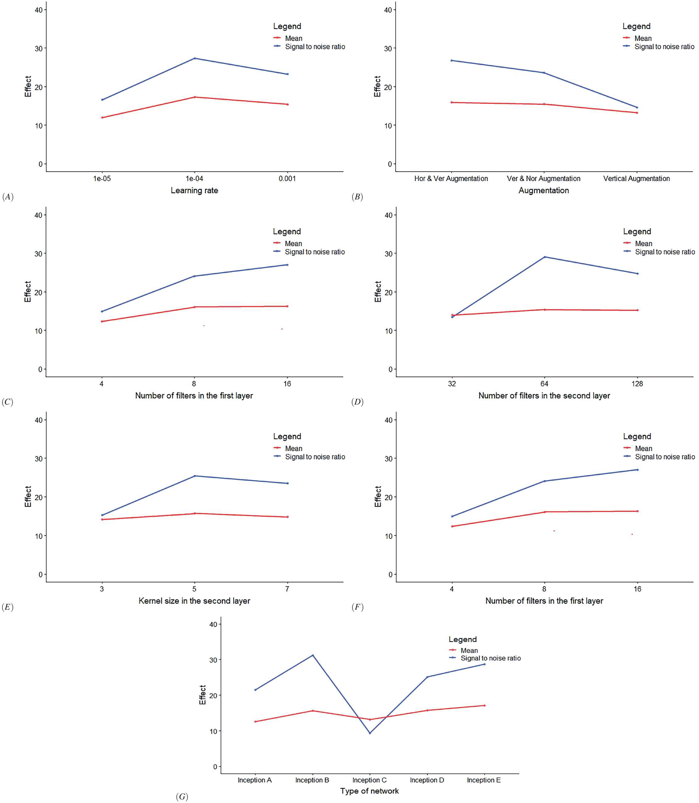
Figure 6 shows the effect plots of mean and signal-to-noise ratio of controlling variables introduced in the first design (DOE for the simple CNN). The first controlling factor was the learning rate. Since the aim of learning rate is to control and adjust the network weights to reduce network loss, having appropriate initial learning rate helps the network to converge faster, hence reducing the computation time. According to the ANOVA, the effect of the learning rate was significant. Similarly, the effect plots demonstrated that the best level of learning rate was 0.0001. For the rest of the DOEs, the best obtained leaning rate was still 0.0001.

Effect plots of mean and signal-to-noise ratio for seven controlling factors of the simple convolutional neural network (CNN) used in the first design. Each plot is for one of the controlling factors, namely: A) Learning rate, B) Type of augmentation, C) Number of filters in the first simple primitive block, D) Number of filters in the second simple primitive block, E) Convolution kernel size in the first block, F) Convolution kernel size in the second block, G) Type of network (Net1 represent the simple CNN without middle fully connected layer and Net2 represent simple CNN with middle fully connected layer).
The next factor investigated was the augmentation type. In the first design, four types of augmentation were selected; vertical, horizontal, vertical and horizontal, and no augmentation. These augmentations were chosen according to the nature of the data. The data applied in the current study were three spectral laser reflectance values (at three different wavelengths) collected by the plant discrimination unit (PDU), PDU collects linearly three laser reflectance values [35]. Accumulation of these linear responses resulted in three layers of two-dimensional inputs. Wild leaf plants (Canola and Radish) were considered as two input classes. Two hundred plants were grown. 2400 spectral data were collected for each plant stage. Data were collected in five different stages, three days after early germination for five consecutive weeks. A total of 12000 data were generated for each class. Sixty percent of the data set was kept for training and the rest was equally divided for validation and testing. Training, validation, and testing plants were kept strictly separated to ensure the generalization of the study. A sample data set used for training is shown in Figure 7. Vertical augmentation changed the order of the laser beams from end to beginning. The horizontal augmentation changed the direction of 2D arrays of data. The results show that the combination of horizontal and vertical augmentation significantly changed the value RPD accuracy.

A sample data used as combination of three-layer laser spectral reflectance.
The role of filters in the first layer was to help learning the basic features and in the following layer and combine these features to produce deep learning according to more complex features. When there were not much basic features in the data, the number of filters in the first layer could be reduced to minimize the computational cost. Results showed that with 16 or 32 filters in the first layer and 128 or 256 filters in the second layer, better RPD accuracy could be obtained. While the difference between the number of filters in the first layer and second layer were not statistically significant, the interaction between the filters in these two layers provided significant differences in RPD accuracy.
The next two controlling factors introduced were the kernel sizes. According to effect plots, there was slight improvement using
In the last controlling factor, the two simple CNNs shown in Figure 4 were compared. One CNN was with two simple blocks and a fully connected layer for classification, while the other CNN with an extra middle fully connected layer, to be able to combine all the extracted feature for classification following ReLu function. The results show that there was no significant difference between these factors, with the CNN without the middle fully connected layer providing better RPD accuracy. This is due to the low number of features in our selected dataset, meaning that when a dataset is simpler according to its number of features, there is no need to make the network more complex and increase the computational expenses.
3.2.2. Design 2
Figure 8 shows effect plots of the means and signal-to-noise ratios for the factors of the second design. As can be seen from Figure 8, the 0.0001 value was still the best for initialization of learning rate. In this design, three types of augmentation were investigated, namely vertical, vertical and normalized, and horizontal and vertical augmentation. Figure 8 clearly shows that using horizontal and vertical augmentation still provided significantly better RPD accuracy in terms of both mean plot and signal-to-noise ratio.
The effect plot of mean and signal-to-noise ratio for the second design. The effect plot of seven variable investigated in here. A) Learning rate, B) Type of augmentation, C) Number of filters used in the first layer, D) Number of filters use in the second layer, E) Convolution kernel size in the first layer, F) Convolution kernel size in the second layer, G) Type of Inception block used in the Inception layer.
Note that while only the number of filters used in the first layer significantly changed the RPD accuracy, the results show that the interaction of the number of filters used in the first layer and the number of filters used in the second were significantly important in the second design based on the use of Inception primitive blocks. This shows that in the second DOE, the combination of features made the second layer more effective in achieving higher accuracy. The optimum number of filters in the first and second layers according to effect plot were 16 and 64, respectively.
According to the mean of effect plots, the best kernel size was
The best RPD accuracy was obtained by the network that used the Inception B block (shown in Table 1), which had the simplest Inception block structure with minimum combination of
3.2.3. Design 3
Figure 9 shows effect plots of the means and signal-to-noise ratios for the factors of the third design. Consistent with previous results, the best learning rate in the third designed network was 0.0001. The augmentation types selected were horizontal, vertical, and horizontal and vertical augmentation. The combination of horizontal and vertical augmentation provided significantly better RPD accuracy since it provided more scenarios for the network learning process.

The effect plot of mean and signal-to-noise ratio for the third design. The variable investigated were A) Learning rate, B) Number of blocks used in the Resnet layers, C) Type of augmentation, D) Number of filters used in the first Resnet layer, E) Number of filters used in the second Resnet layer, F) Convolution kernel size in the first Resnet layer, G) Convolution kernel size in the second Resnet layer.
In each residual layer, the effects of using various numbers of residual blocks were investigated to determine the importance of going deeper for classification. The results showed that the best mean RPD accuracy was obtained by using four blocks, while the difference of using various blocks were not statistically significant. The other insignificant parameters here were the number of filters and kernel sizes. As can be seen from Figure 9, the difference between the means of RPD accuracy was insignificant. This is because when the residual layer can learn from the previous layer and possesses a low number of features, it does not required more filters. Instead, one can go deeper and use the residual layers, which make the effect of number of filters and kernel sizes less important for a dataset of low features. Therefore, in this case, the minimum level of filters can be selected to reduce the computational cost.
3.2.4. Design 4
Figure 10 shows effect plots of the means and signal-to-noise ratios for the factors of the comparison design. In the last DOE, three designed CNNs were compared. The best learning rate obtained was 0.0001, which was in accordance with the previous results. The variations between using various augmentations were slight, while the vertical and horizontal augmentation resulted in an acceptable signal-to-noise ratio and a mean effect plot. According to the effect plots, a suitable number of filter size can be chosen, 16 for the first layer and 64 for the second layer. While the impact of each filter was not statistically significant, the interaction between them showed that in order to have proper feature extraction, the interaction between filters is important. Based on the effect plots, the optimum kernel sizes was
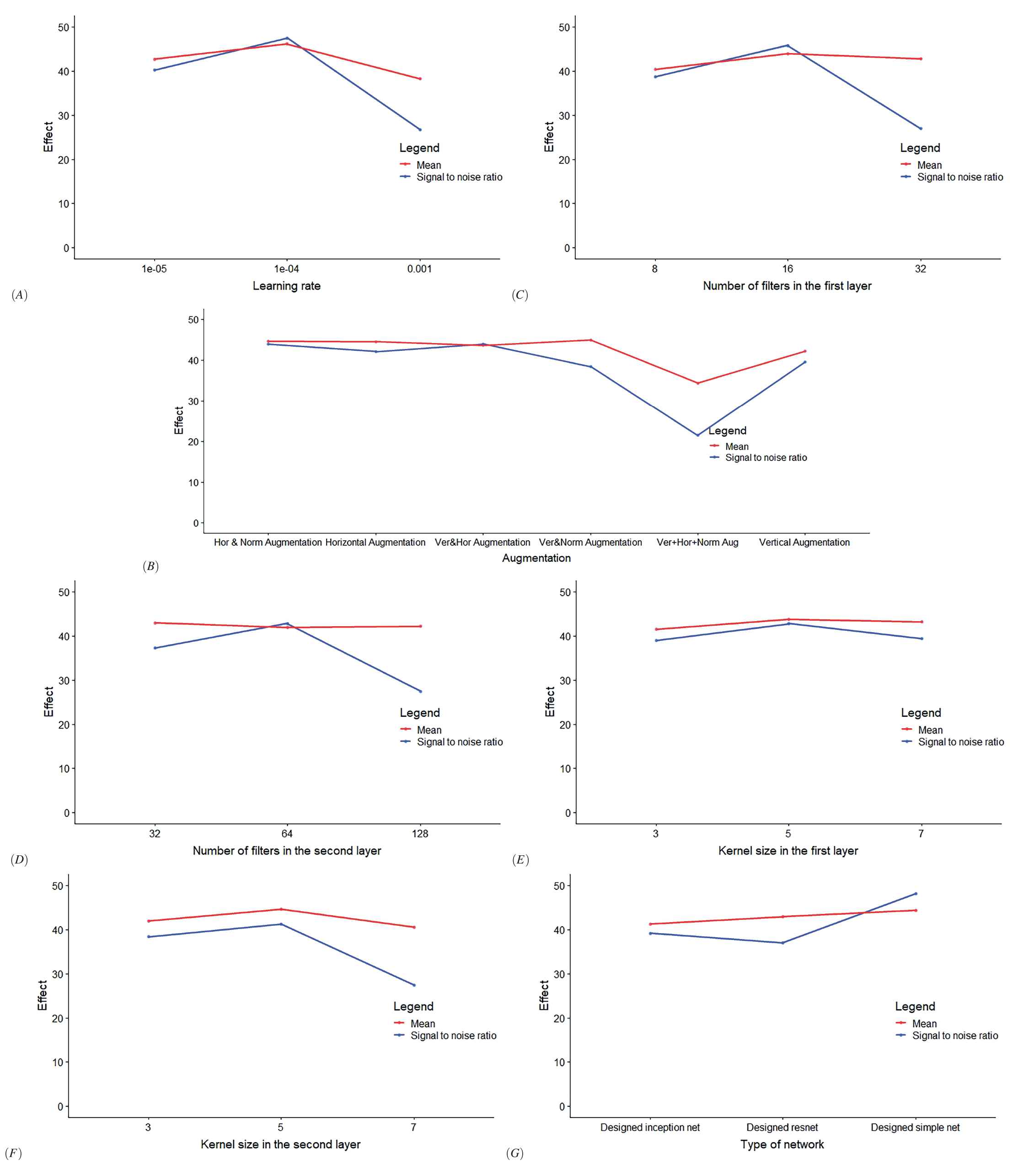
The effect plots of mean and signal-to-noise ratio of the fourth design for comparison of designed simple convolutional neural network (CNN), designed Inception net, and designed Resnet. Each plot belong to one of the controlling variable namely: A) Learning rate, B) Type of augmentation, C) Number of filters in the first primitive block, D) Number of filters in the second primitive block, E) Convolution kernel size in the first block, F) Convolution kernel size in the second block, G) Type of network (designed Inception, designed Resnet, designed simple net).
3.3. Comparison of CNNs with and without Optimizations
The aim of the last investigation was to introduce an approach that determines the simplest network that could be classified as efficient as the manually-engineered network. The previously-discussed agricultural dataset was also chosen to evaluate the optimization procedure. The designed CNNs were compared based on their testing accuracies before and after parameter optimization. In order to have better comparison, the network was activated with five various seeds, namely cuda and pytorch random seeds. Figure 11 shows the average testing accuracies of the investigated CNNs activated with five different random seeds. The comparison results show that, for all the cases, there were improvements in the testing accuracy. Generally, there was a correlation between the number of significant controlling factors in the optimization process and the amount of improvement in accuracy. The Inception network had five significant controlling factors, resulting in the highest improvement in accuracy, while the Resnet network had only three significant factors, displaying the lowest improvement in accuracy Tables 6–9.

Average testing accuracies of the convolutional neural networks (CNNs) activated with five different random seed.
| Df | Sum Sq | Mean Sq | F value | Pr( |
|
|---|---|---|---|---|---|
| Learning rate | 1 | 21387.0 | 21387.0 | 240.3860 | |
| Augmentation | 1 | 1201.2 | 400.4 | 4.5005 | 0.006079 ** |
| Number of filters in the first block | 1 | 524.0 | 524.0 | 5.8902 | 0.017841 * |
| Number of filters in the second block | 1 | 33.1 | 33.1 | 0.3722 | 0.543827 |
| Kernel size in block 1 | 1 | 8.0 | 8.0 | 0.0895 | 0.765775 |
| Kernel size in block 2 | 1 | 100.4 | 100.4 | 1.1282 | 0.291857 |
| Type of network | 1 | 2.3 | 2.3 | 0.0264 | 0.871462 |
| Interaction between filters | 1 | 556.4 | 556.4 | 6.2541 | 0.014769 * |
| Residuals | 69 | 6138.9 | 88.96 |
DOE = design of experiment; Signif. codes; 0 ‘***’ 0.001 ‘**’ 0.01 ‘*’ 0.05 ‘.’ 0.1 ‘ ’ 1.
Analysis of variance for comparing factors according to the first DOE, the response was the relative percentage difference in accuracy.
| Df | Sum Sq | Mean Sq | F value | Pr( |
|
|---|---|---|---|---|---|
| Learning rate | 1 | 24.53 | 24.53 | 1.5470 | 0.217459 |
| Augmentation | 2 | 123.43 | 61.71 | 3.8914 | 0.024664 * |
| Number of filters in the first block | 1 | 175.63 | 175.63 | 11.0742 | 0.001358 ** |
| Number of filters in the second block | 1 | 14.73 | 14.73 | 0.9290 | 0.338209 |
| Kernel size in block 1 | 1 | 71.95 | 71.95 | 4.5366 | 0.036458 * |
| Kernel size in block 2 | 1 | 6.71 | 6.71 | 0.4231 | 0.5173687 |
| Type of network | 1 | 221.46 | 44.29 | 2.7928 | 0.022859 * |
| Interaction between filters | 1 | 120.34 | 120.34 | 7.5881 | 0.007369 ** |
| Residuals | 75 | 1189.45 | 15.86 |
DOE = design of experiment; Signif. codes: 0 ‘***’ 0.001 ‘**’ 0.01 ‘*’ 0.05 ‘.’ 0.1 ‘ ’ 1.
Analysis of variance for comparing factors according to the second DOE, the response was the relative percentage difference in accuracy.
| Df | Sum Sq | Mean Sq | F value | Pr( |
|
|---|---|---|---|---|---|
| Learning rate | 1 | 5655.7 | 5655.7 | 50.4665 | 4.245e-10 *** |
| Augmentation | 2 | 974.0 | 487.0 | 4.3456 | 0.01612 * |
| Number of filters in the first block | 1 | 12.0 | 12.0 | 0.1067 | 0.74481 |
| Number of filters in the second block | 1 | 72.9 | 72.9 | 0.6504 | 0.42232 |
| Kernel size in block 1 | 1 | 22.2 | 22.2 | 0.1978 | 0.65772 |
| Kernel size in block 2 | 1 | 361.8 | 361.8 | 3.2281 | 0.07611 |
| Resnet blocks | 1 | 20.0 | 20.0 | 0.1783 | 0.67392 |
| Residuals | 81 | 9077.5 | 112.1 |
DOE = design of experiment; Signif. codes: 0 ‘***’ 0.001 ‘**’ 0.01 ‘*’ 0.05 ‘.’ 0.1 ‘ ’ 1.
Analysis of variance for comparing factors according to the third DOE, the relative percentage difference in accuracy was considered as response.
| Df | Sum Sq | Mean Sq | F value | Pr( |
|
|---|---|---|---|---|---|
| Learning rate | 1 | 689.74 | 689.74 | 22.4571 | 9.973e-06 *** |
| Augmentation | 5 | 1234.51 | 246.90 | 8.0388 | 4.122e-06 *** |
| Number of filters in the first block | 1 | 57.39 | 57.39 | 1.8685 | 0.175736 |
| Number of filters in the second block | 1 | 3.45 | 3.45 | 0.1123 | 0.738422 |
| Kernel size in block 1 | 1 | 43.93 | 43.93 | 1.4304 | 0.234546 |
| Kernel size in block 2 | 1 | 30.04 | 30.04 | 0.9780 | 0.325866 |
| Type of network | 2 | 439.45 | 219.72 | 7.1539 | 0.001434 ** |
| Interaction between filters | 1 | 250.80 | 250.80 | 8.1659 | 0.005522 ** |
| Residuals | 75 | 2303.52 | 30.71 |
DOE = design of experiment; Signif. codes: 0 ‘***’ 0.001 ‘**’ 0.01 ‘*’ 0.05 ‘.’ 0.1 ‘ ’ 1.
Analysis of variance for comparing factors according to the fourth DOE, the relative percentage difference in accuracy was considered as response.
4. CONCLUSION
In this paper, four main DOE have been proposed and investigated to determine and optimize the significant factors that affect the performance of three simplified CNN architectures, namely, the VGG network, the Inception network, and the Resnet network. DOE algorithms based on utilizing Taguchi statistical methods have been developed for optimizing CNN parameters, and then tested using spectral agricultural data. Results have shown that, for all investigated CNN architectures, there was measurable improvement in accuracy in comparison with un-optimized CNNs, and that the Inception network yields the highest improvement (
CONFLICT OF INTEREST
Authors have no conflict of interest to declare.
ACKNOWLEDGMENTS
The research is supported by Edith Cowan University, the Grains Research and Development Corporation (GRDC), Australian Research Council, Photonic Detection Systems Pty. Ltd, Australia, and Pawsey Supercomputing Centre.
REFERENCES
Cite this article
TY  - JOUR
AU  - Saman Akbarzadeh
AU  - Selam Ahderom
AU  - Kamal Alameh
PY  - 2019
DA  - 2019/12/23
TI  - A Statistical Approach to Provide Explainable Convolutional Neural Network Parameter Optimization
JO  - International Journal of Computational Intelligence Systems
SP  - 1635
EP  - 1648
VL  - 12
IS  - 2
SN  - 1875-6883
UR  - https://doi.org/10.2991/ijcis.d.191219.001
DO  - 10.2991/ijcis.d.191219.001
ID  - Akbarzadeh2019
ER  -