
Enhanced Particle Swarm Optimization Based on Reference Direction and Inverse Model for Optimization Problems
- DOI
- 10.2991/ijcis.d.200127.001How to use a DOI?
- Keywords
- Particle swarm optimization; Reference direction; Non-dominated sorting; Inverse model; Neural networks optimization
- Abstract
While particle swarm optimization (PSO) shows good performance for many optimization problems, the weakness in premature convergence and easy trapping into local optimum, due to the ignorance of the diversity information, has been gradually recognized. To improve the optimization performance of PSO, an enhanced PSO based on reference direction and inverse model is proposed, RDIM-PSO for short reference. In RDIM-PSO, the reference particles which are used as reference directions are selected by non-dominated sorting method according to the fitness and diversity contribution of the population. Dynamic neighborhood strategy is introduced to divide the population into several sub-swarms based on the reference directions. For each sub-swarm, the particles focus on exploitation under the guidance of local best particle with a good guarantee of population diversity. Moreover, Gaussian process-based inverse model is introduced to generate equilibrium particles by sampling the objective space to further achieve a good balance between exploration and exploitation. Experimental results on CEC2014 test problems show that RDIM-PSO has overall better performance compared with other well-known optimization algorithms. Finally, the proposed RDIM-PSO is also applied to artificial neural networks and the promising results on the chaotic time series prediction show the effectiveness of RDIM-PSO.
- Copyright
- © 2020 The Authors. Published by Atlantis Press SARL.
- Open Access
- This is an open access article distributed under the CC BY-NC 4.0 license (http://creativecommons.org/licenses/by-nc/4.0/).
1. INTRODUCTION
With the development of science and technology, there are more and more optimization problems encountered in science and engineering fields. Without loss of generality, a numerical optimization problem can be defined as follows.
Evolution-based, physics-based and swarm intelligence-based methods [3] are three main categories for nature-inspired optimization algorithms. Genetic algorithm (GA) [4], genetic programming (GP) [5], differential evolution (DE) [6] and derandomized evolution strategy with covariance matrix adaptation (CMA-ES) [7], can be seen as evolution-based optimization algorithms because they are inspired by the laws of biological evolutionary process. Simulated annealing (SA) [8], chemical reaction optimization (CRO) [9], fireworks algorithm (FA) [10] and brain storm optimization (BSO) [11], can be seen as physics-based optimization algorithms because they imitate the physical or natural phenomena in the universe. Particle swarm optimization (PSO) [12], artificial bee colony (ABC) [13], teaching–learning-based optimization (TLBO) [14] and whale optimization algorithm (WOA) [3], can be seen as swarm intelligence-based methods because they mimic the social behavior of all kinds of animals.
In 1995, Kennedy and Eberhart [12] introduced an effective optimizer called PSO. The algorithm mimics the flocking behavior of birds. The PSO method is successfully applied in solving real-world engineering problems because of its better computational efficiency. However, rapid convergence and diversity loss make traditional PSO encounter premature convergence for solving complex optimization problems [15]. Moreover, how to achieve a fine balance between exploration and exploitation remains a big challenge. Over the past decades, a number of methods have been developed for speeding up convergence and alleviate premature convergence. Recently, the popular methods are inverse modeling, reference directions, cooperative approach [16], social learning approach [17], etc. The inverse modeling approach [18] creates offspring by sampling the objective space to improve the search performance of the algorithm. The reference direction method splits the objective space into a number of independent subregions, helping guide the search toward the optimal solution with a good guarantee of population diversity [19]. To our knowledge, inverse modeling approach and the reference direction method are mainly used to solve multiobjective optimization problems. Therefore, this paper attempts to apply inverse model and reference direction to improve the performance of PSO (RDIM-PSO) for solving single-objective optimization problems.
The main contributions of this paper are summarized as follows:
Non-dominated sorting mechanism which takes into account the population fitness and diversity contribution is introduced to select reference particles during optimization search. The main purpose of doing so is to construct a dynamic neighborhood model which encourages the RDIM-PSO to explore the local optimum area and the sparse region.
Inverse model is introduced to produce equilibrium particles at each generation, which helps the population balance the exploration and exploitation abilities effectively.
A new velocity updating strategy is proposed, whose major role is to achieve fast and accurate convergence.
Systematic experiments conducted to compare RDIM-PSO with seven state-of-the-art evolutionary algorithms (EAs) on CEC2014 test problems and three application problems of artificial neural network (ANN) are described. The experimental results show that the proposed method is promising for solving optimization problems.
The remainder of this paper is organized as follows. In Section 2, the basic idea of PSO and related work are reviewed. In Section 3, the proposed RDIM-PSO is presented in detail. Section 4 reports and discusses the experimental results. In Section 5, RDIM-PSO is applied to three application problems of ANN. Finally, the conclusions and possible future research are drawn up in Section 6.
2. PSO AND RELATED WORK
2.1. PSO Algorithm
In PSO algorithm, each particle i represents a potential solution. The velocity
To restrict the change of velocities, Shi and Eberhart introduced an inertia weight [20].
The inertia weight ω is computed as follows:
Algorithm 1: Particle Swarm Optimization (PSO)
1: Initialize parameters and population
2: Evaluate the population
3: Compute pbesti (i = 1,2,…, PopSize) and gbest
4: while the termination criteria are not met do
5: for i = 1 to PopSize do
6: Update vi and xi
7: Evaluate xi
8: Update pbesti and gbest
9: end for
10: end while
Output: the particle with the smallest objective function value in the population.
2.2. Related Work
Traditional PSO cannot effectively solve complex optimization problems. Then, variants of modified PSOs are proposed to improve the performance of PSO. The improvements can be divided into three categories.
Improvements of the control parameters [20–24]. Inertia weight is introduced in [20] to restrict the change of velocities and control the scope of search. To guarantee convergence and encourage exploration, PSO with constriction factor (PSOcf) is designed in [21]. Nobile et al. [22] introduces fuzzy self-turning PSO (FST-PSO) which uses fuzzy logic to obtain the control parameters used by each particle. Multiple adaptive methods are introduced into PSO in [23] to adaptively control the parameters. A chaotic map and dynamic weight are introduced in PSO to modify the search process [24].
Improvements of the evolutionary learning strategy [25–31]. The learning strategy algorithm (CLPSO) is designed to adjust the velocity of the particles and solve premature in [25]. To guide the particles to fly in better directions, a much promising and efficient exemplar is constructed by introducing orthogonal learning strategy (OLPSO) in [26]. Quyang et al. [27] presents the idea of an improved global-best-guided (IGPSO) to enhance the exploitation ability of the algorithm. In IGPSO, optimization strategies include the global neighborhood strategy, the local learning strategy, stochastic learning strategy and opposition based learning strategy are employed to improve the optimization potential of PSO. Two kinds of PSO, namely a surrogate-assisted PSO and a surrogated-assisted social learning-based PSO, worked together to search the global optimum [28]. To ensure the swarm diversity and fast convergence, the idea of all-dimension-neighborhood-based and randomly selected neighbors learning strategy is introduced in PSO (ADN-RSN-PSO) [29]. For updating particle velocity, Wang et al. employed a dynamic tournament topology strategy [30] while Jensi et al. introduced a levy flight method [31].
Neighborhood-based strategies [32–38]. Neighborhood strategy has been widely used because it can effectively improve the performance of EAs. An index-based neighborhood strategy is employed in fully informed PSO [32]. The neighborhood operator, which is used to adjust the local neighborhood size, is introduced in [33]. A dynamic neighborhood learning strategy (DNLPSO), proposed by Nasir et al., is introduced in [34]. In DNLPSO, the exemplar particle is selected from a neighborhood, and the learner particle learns the historical information from its neighborhood. The idea of multi-swarm and dynamic learning strategy (PSO-DLS) is introduced in [35]. In PSO-DLS, the population is divided into several sub-swarms. In each sub-swarm, the task of ordinary particles is to search a better lbest. The cyclic neighborhood topology strategy (CNT-CPSO), proposed by Maruta et al., is introduced in [36]. Specifically, the cyclic-network topology is employed to construct neighborhood structure for each particle. The idea of cluster is employed to enhance the performance of PSO (pkPSO) in [37]. In [37], the particles, which are clustered on the Euclidean spatial neighborhood structure, explore the promising areas and obtain better solutions. A hybrid PSO algorithm (DNSPSO), which employs two strategies, namely diversity enhancing strategy and neighborhood strategy, is proposed in [38]. A trade-off between exploration and exploitation abilities is achieved with the two strategies.
3. ENHANCED PSO BASED ON REFERENCE DIRECTION AND INVERSE MODEL
It is known that better optimization performance can be achieved by the proper balance between global exploration and local exploitation. In order to further improve the performance of PSO, three major changes are proposed in RDIM-PSO. The first change is the construction of the dynamic neighborhood model. The diversity and the fitness of the particle are considered as a two-objective problem. Then, the non-dominated sorting mechanism is employed to select the reference particles which are considered as the reference directions. Next, the population is partitioned into several independent sub-swarms (neighborhood) with reference particles. The second change is the utilization of the inverse model. The samples are generated with reference particles in the objective space. The inverse models are employed to map the samples back to the decision space. The equilibrium particles which are generated by the inverse models can balance the exploration and exploitation. The last change is the introduction of a new velocity update strategy which is used to improve the performance of the proposed algorithm.
3.1. Dynamic Neighborhood Strategy
In the classical PSO, the personal best experience (pbest) and the global best experience (gbest) are used to adjust the flying trajectory of each particle. However, if the current gbest is far from the global optimum, particles may easily get trapped in a local optimum because of misleading from the current gbest [25]. In order to achieve better performance, PSO should establish a good balance between exploration and exploitation. Related works show that the multi-swarm can discourage premature convergence and maintain the diversity in some extent [16,34,39]. There are various types of topology can be used for the implementation of the neighborhood, such as star, wheel, circular, pyramid and 4-clusters [21]. The division of sub-swarm is usually based on index or fitness values [24,35,40,41]. In RDIM-PSO, non-dominated sorting procedure which comes from non-dominated sorting genetic algorithm II (NSGA-II) [42] is employed to realize the dynamic division of neighborhood.
NSGA-II is a classical multiobjective optimization algorithm. It is necessary to note that the conflicting objectives are the prerequisite for the multiobjective optimization problems. The major problem of the optimization algorithm is the balance between the exploration and exploitation. However, the exploration and the exploitation are the conflicting objectives. Generally, the exploration efficiency is depended on the distribution of particles, namely population diversity, while the exploitation efficiency is associated with the fitness of particles. Then, diversity and fitness can be used to indirectly measure the exploration and exploitation, respectively. In view of this idea, NSGA-II can be employed after constructing two objectives, diversity and fitness.
The diversity measures reported in the literature can be largely classified into two categories, namely the diversity contribution measure on whole population level and on individual level, respectively. Here, the diversity for a single particle to whole population is defined based on Euclidean distance.
As mentioned before, two conflicting objectives should be constructed before employing non-dominated sorting procedure. The better the diversity of population is, the stronger the ability of exploration is. The better the fitness of the population is, the stronger the exploitation ability is. In this paper, population diversity is directly proportional to the diversity value, while population fitness is inversely proportional to the objective function value. In order to utilize the non-dominated sorting procedure, the objective functions are transformed into the minimization optimization problem. In addition, in order to ensure that the values of the fitness and the diversity are in the same range, two objectives, fitness and diversity, associated with each particle in the population can be calculated as
The reference particles are selected by non-dominated sorting procedure. The motivation behind the idea of applying the selective strategy on the reference particles is that diversity and fitness can be employed to achieve a trade-off between exploration and exploitation [43]. Details of the fast-non-dominated-sort algorithm can be found in [42]. Figure 1 shows the output of non-dominated sorting procedure. The particles in the lowest layer belong to front 1. The reference particles
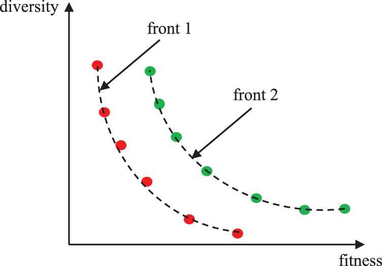
Output of the non-dominated sorting procedure.
In RDIM-PSO, the reference particles which have a good guarantee of population diversity are employed to divide the population into several independent sub-swarms, namely neighborhoods. Each particle is associated with a specific reference particle according to its positions in the search space. More exactly, an arbitrary particle

Relation between a particle and a reference particle.
3.2. Equilibrium Particles Generation Strategy
As mentioned above, the reference particles have a good guarantee of population diversity. Then, a Gaussian process-based inverse model [18] is constructed to map all reference particles found so far from the objective space to the decision space at every generation. Like reference particles, the mapped particles which called equilibrium particles have better fitness and diversity. At each generation, randomly selected particles are replaced by the equilibrium particles. In doing so, the exploration and exploitation abilities can be balanced effectively.
Details of Gaussian process-based inverse model can be found in [18]. First, the reference particles are used for training two groups of inverse models. The training data set for training the inverse model
Second, the test input
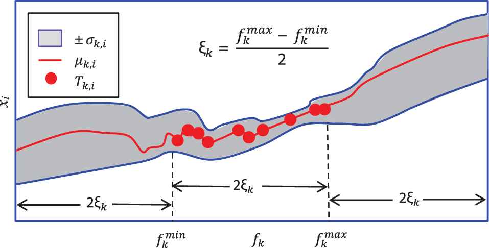
Gaussian process-based inverse model.
Finally, the test input
3.3. Velocity Update Strategy
As mentioned above, the dynamic neighborhood strategy based on reference particles is employed to divide the population into different sub-swarms. The sub-swarm guided by the reference particle which has better fitness but worse diversity undertakes the task of exploitation. The sub-swarm guided by the reference particle which has worse fitness but better diversity is responsible for the exploration task. The sub-swarm guided by the reference particle which has medium fitness and diversity contributes to balancing between exploration and exploitation. The velocity of RDIM-PSO is updated according to the following equation:
3.4. Complexity Analysis of RDIM-PSO
In RDIM-PSO, the computational costs involve the initialization (Ti), evaluation (Te), non-dominated sorting procedure (Ts), velocity (Tv), Gaussian process-based inverse model (Tgp) and position (Tp), for each particle. As mentioned in [43], the time complexity of the non-dominated sorting procedure is O(M × N2), where M is the number of objectives and N is the population size. Therefore, the total time complexity of RDIM-PSO can be estimated as follows:
D represents the dimension of the search space. Therefore, the time complexity of the proposed algorithm is
Based on the above explanation, the pseudo-code of the RDIM-PSO algorithm is illustrated in Algorithm 2. rand denotes a random number from (0, 1]. rand (K) denotes K random numbers from (0, 1]. x* denotes a particle reproduced with inverse model.
Algorithm 2: RDIM-PSO algorithm
1: Initialize D(number of dimensions), N
2: Initialize position xi, velocity vi of the N particles (i = 1, 2, …, N)
3: Compute the objective function value and diversity of each particle according to (8) and (9)
4: Set pbesti and gbest of the N particles (i = 1, 2, …, N)
5: Find the particles in the first non-dominated front with the non-dominated sorting procedure
6: Compute reference particles according to (10)
7: Partition the population by K reference particles according to (11)
8: Inverse Modeling: build inverse models and training a Gaussian process for each inverse model according to (12) and (13)
9: Reproduction: reproduce K particles by sampling the objective space and mapping them back to the decision space using the inverse models according to (14)
10: while the termination criteria are not met do
11: Compute inertia weight ω according to (5)
12: Set nbestj of the K sub-swarms (j = 1, 2,…, K)
13: for i = 1 to N do
14: Update the velocity vi according to (15)
15: Update the position xi according to (3)
16: end for
17: if rand <= 1/N
18: index =
19:
20: end if
21: Calculate objective function value of each particle
22: for i = 1 to N do
23: if xi is better than pbesti
24: pbesti = xi
25: end if
26: if xi is better than gbest
27: gbest = xi
28: end if
29: end for
30: Compute the diversity of each particle according to (9)
31: Find the particles in the first non-dominated front with the non-dominated sorting procedure
32: Compute reference particles according to (10)
33: Partition the population by K reference particles according to (11)
34: Inverse Modeling: build inverse models and training a Gaussian process for each inverse model according to (12) and (13)
35: Reproduction: reproduce K particles by sampling the objective space and mapping them back to the decision space using the inverse models according to (14)
36: end while
Output: the particle with the smallest objective function value in the population.
To evaluate the performance of several components introduced in RDIM-PSO, RDIM-PSO is compared with PSO-N, PSO-NV and PSO-w on f3, f4, f17 and f29 with D = 30. Based on PSO-w, we introduce dynamic neighborhood strategy to achieve PSO-N. Based on PSO-N, we introduce velocity update strategy to achieve PSO-NV. Based on PSO-NV, we introduce Gaussian process-based inverse model to achieve RDIM-PSO. Four representative problems including unimodal problem (f3), simple multimodal problem (f4), hybrid problem (f17) and the composite problem (f29) are selected. The convergence curves in Figure 4 illustrate mean errors (in logarithmic scale) in 30 independent simulations of PSO-w, PSO-N, PSO-NV and RDIM-PSO. The mean error is defined as f(x)-f(x*). f(x) is the best fitness value and f(x*) is the real global optimization value. The termination criterion is decided by the maximal number of function evaluations (MaxFES), which is set to 30,000.
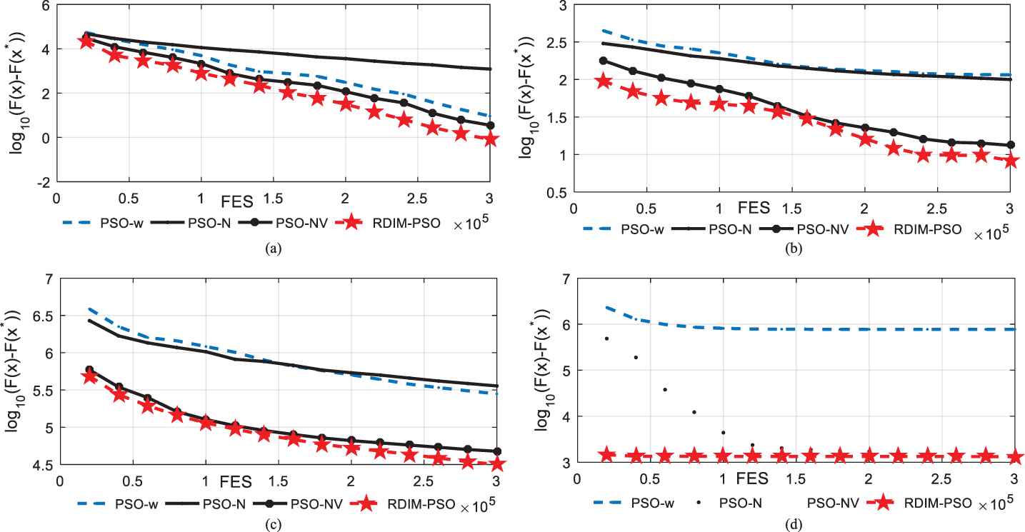
Evolution of the mean function error values derived from PSO-w, PSO-N, PSO-NV and RDIM-PSO versus the number of FES on four test problems with D = 30. (a) f3; (b) f4; (c) f17; (d) f29.
Figure 4 shows that PSO-N performs worse on unimodal problem compared PSO-w, while it performs better on simple multimodal problem and composite problem. The reason is that the neighborhood strategy is suitable for solving these problems. The velocity update strategy can improve the convergence rate. Then, PSO-NV converge faster than PSO-N and PSO-w on f3, f4, f17 and f29. Gaussian process-based inverse model is helpful for balancing the exploration and exploitation. Then, RDIM-PSO performs better than these compared algorithms because of introducing three improvement strategies into PSO.
4. EXPERIMENTS AND DISCUSSIONS
In this section, CEC2014 contest benchmark problems, which are widely adopted in numerical optimization methods, are used to verify the performance of RDIM-PSO. The general experimental setting is explained in Section 4.1. The experimental results and comparison with other algorithms are explained in Section 4.2.
4.1. General Experimental Setting
Thirty benchmark problems proposed in the special session on real-parameter optimization of CEC2014 [35] are used to evaluate the performance of RDIM-PSO in our experiments. The search ranges of all the test problems are [−100, 100]D. CEC2014 contest benchmark problems are divided into four groups according to their diverse characteristics. In this paper, fi denotes the ith benchmark problem, that is, optimization function. The first group includes three unimodal problems f1– f3. The second group includes 13 simple multimodal problems f4– f16. The third group includes six hybrid problems f17– f22. The fourth group includes eight composite problems f23– f30. The details of these benchmark problems can be found in [35]. In this paper, seven algorithms are selected to compare with the proposed algorithm. These algorithms can be divided into three categories. PSO-w, SLPSO belongs to the category of improving the control parameters. CLPSO, TLBO, CSO and Jaya belong to the category of improving the evolutionary learning strategy. CPSO-H belongs to the category of neighborhood-based strategies.
The compared algorithms and parameters settings are listed below:
PSO with inertia weight (PSO-w) [20];
Cooperative particle swarm optimizer (CPSO-H ) [16];
Comprehensive learning particle swarm optimizer (CLPSO) [25];
Social learning PSO (SLPSO) [17];
Teaching–learning-based optimization (TLBO) [14];
Competitive swarm optimizer (CSO) [44];
Jaya (a Sanskrit word meaning victory) algorithm [45];
RDIM-PSO.
The performance of the algorithm can be affected by its population size. Generally, larger population is needed to enhance exploration at the beginning of the search, while at the end of the search, smaller population is needed to enhance exploitation. However, it is well-known that the loss of population diversity may result into premature convergence while and excessive diversity may cause stagnation [46]. In this paper, the population size of each compared algorithm is refer to the original paper. For PSO-w, CPSO-H and SLPSO, the population size is set to 20 [16,17,20]. For CLPSO, Jaya and RDIM-PSO, the population size is set to 40 [25,45]. For TLBO and CSO, the population size is set to 100 [14,44]. To make a fair comparison, the termination criterion for all algorithms is decided by the maximal number of function evaluations (MaxFES), which is set to D × 10,000. The dimension (D) is set to 30, 50 and 100, respectively.
Furthermore, the metrics, such as Fmean (mean value), SD (standard deviation), Max (maximum value) and Min (minimum value) of the solution error measure [47], are used to appraise the performance of each algorithm. The solution error measure is defined as f(x)–f(x*). f(x) is the best fitness value and f(x*) is the real global optimization value. The smaller the solution error is, the better the solution quality is. To make a clear comparison, the error is assumed to be 0 when the value f(x)–f(x*) is less than 10−8. In view of statistics, the Wilcoxon signed-rank test [48] at the 5% significance level is used to compare RDIM-PSO with other compared algorithms. “≈”, “
To obtain an unbiased comparison, all the experiments are run on a PC with an Intel Core i7-3770 3.40 GHz CPU and 4 GB memory. All experiments were run 30 times, and the codes are implemented in Matlab R2013a.
4.2. Comparison with Eight Optimization Algorithms
Before comparing with other algorithms, f1 is used as an example to show the major process of the proposed algorithm. We select the first two dimensions of the particles for clarity. First, initialize the population. For each generation cycle, we sort the population according to the fitness and diversity of each particle using the non-dominated sorting procedure. The reference particles is generated according to formula (10). Figure 5(a) shows the first two dimensions of reference particles. Next, the population is divided into several neighborhoods by these reference particles. The neighborhood size is equal to the number of the reference particles. The inverse models are built and a Gaussian process is trained for each inverse model. For each reference particle, an offspring is reproduced by sampling the objective space and mapping them back to the decision space using the inverse model. Figure 5(b) shows the offspring generated by the inverse model. In addition, for each sub-swarm, the best particle is selected as nbest. Then, the velocity and the position of each particle are updated. When the given criteria is satisfied, the randomly selected particles are replaced by the offspring which are generated by the inverse models. Next, the pbest for each particle and the gbest are updated. Figure 5(c) shows the updated particle (pbest). The optimal solution is achieved when the termination criteria are met.
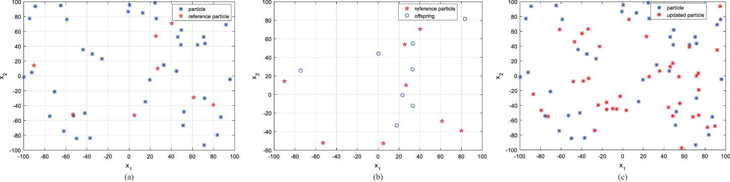
Major optimization process of RDIM-PSO.
(1) Unimodal problems f1–f3
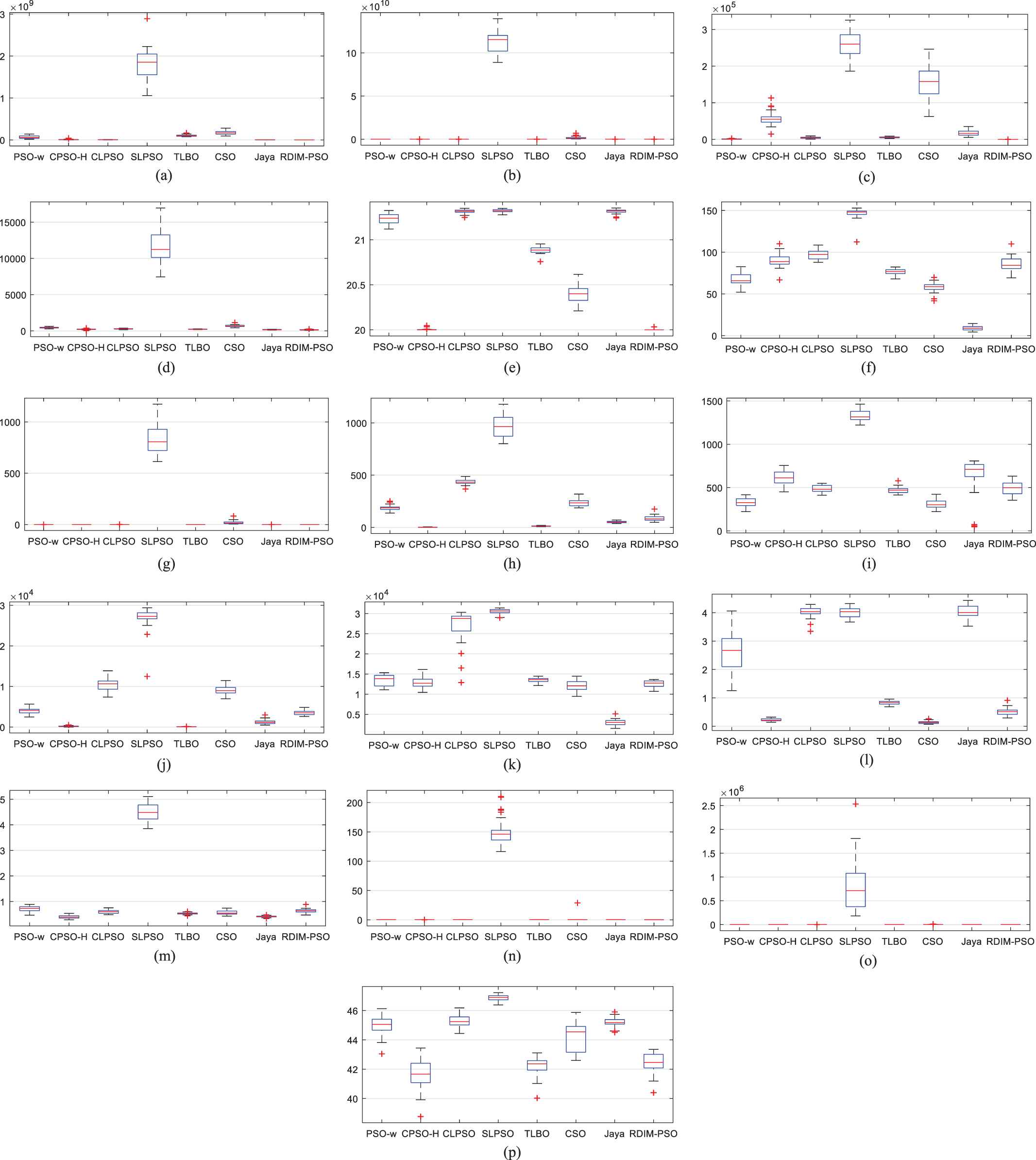
From the statistical results of Table 1, we can see that RDIM-PSO performs well on f1–f3 when D = 30. In case of f1–f3, the results show that RDIM-PSO significantly outperforms PSO-w, CPSO-H, CLPSO, SLPSO, TLBO, CSO and Jaya on 2, 3, 3, 3, 3, 3 and 3 test problems, respectively. The overall Wilcoxon ranking sequences for the test problems are RDIM-PSO, PSO-w, TLBO, CSO, CPSO-H (CLPSO), SLPSO and Jaya in a descending direction. The average rank of CPSO-H is the same as that of CLPSO. Table 2 shows that RDIM-PSO achieves better results on f1–f3 under D = 50. RDIM-PSO outperforms PSO-w, CPSO-H, CLPSO, SLPSO, TLBO, CSO and Jaya on 3, 3, 3, 3, 3, 3 and 3 test problems, respectively. The overall Wilcoxon ranking sequences for the test problems are RDIM-PSO, TLBO (CSO), PSO-w, CPSO-H, CLPSO, SLPSO and Jaya in a descending direction. The average rank of TLBO is the same as that of CSO. Table 3 shows that RDIM-PSO outperforms PSO-w, CPSO-H, CLPSO, SLPSO, TLBO, CSO and Jaya on 2, 2, 2, 3, 2, 2 and 3 test problems under D = 100, respectively. The overall Wilcoxon ranking sequences for the test problems are RDIM-PSO, TLBO, PSO-w (CSO), CPSO-H (CLPSO), SLPSO and Jaya in a descending direction. The average rank of PSO-w is the same as that of CSO. The average rank of CPSO-H is the same as that of CLPSO. For solving unimodal problems, more exploitation is beneficial. RDIM-PSO employs the reference directions to divide the population into several sub-swarms. Each sub-swarm effectively employs neighborhood information to improve local exploitation ability. Thus, RDIM-PSO can find better results for unimodal problems compared with other optimization algorithms.
| F | PSO-w | CPSO-H | CLPSO | SLPSO | TLBO | CSO | Jaya | RDIM-PSO | |
|---|---|---|---|---|---|---|---|---|---|
| Compare/rank | f1 | −/4 | −/5 | −/6 | −/7 | −/3 | −/2 | −/8 | |
| f2 | ≈/1 | −/5 | −/6 | −/7 | −/3 | −/4 | −/8 | ||
| f3 | −/2 | −/6 | −/4 | −/7 | −/3 | −/5 | −/8 | ||
| −/≈/+ | 2/1/0 | 3/0/0 | 3/0/0 | 3/0/0 | 3/0/0 | 3/0/0 | 3/0/0 | ||
| Avg-rank | 2.33 | 5.33 | 5.33 | 7.00 | 3.00 | 3.67 | 8.00 | 1.00 |
Experimental results of PSO-w, CPSO-H, CLPSO, SLPSO, TLBO, CSO, Jaya and RDIM-PSO on f1–f3 with D = 30.
| F | PSO-w | CPSO-H | CLPSO | SLPSO | TLBO | CSO | Jaya | RDIM-PSO | |
|---|---|---|---|---|---|---|---|---|---|
| Compare/rank | f1 | −/4 | −/5 | −/6 | −/7 | −/3 | −/2 | −/8 | |
| f2 | −/5 | −/4 | −/6 | −/7 | −/3 | −/2 | −/8 | ||
| f3 | −/2 | −/6 | −/4 | −/7 | −/3 | −/5 | −/8 | ||
| −/≈/+ | 3/0/0 | 3/0/0 | 3/0/0 | 3/0/0 | 3/0/0 | 3/0/0 | 3/0/0 | ||
| Avg-rank | 3.67 | 5.00 | 5.33 | 7.00 | 3.00 | 3.00 | 8.00 | 1.00 |
Experimental results of PSO-w, CPSO-H, CLPSO, SLPSO, TLBO, CSO, Jaya and RDIM-PSO on f1–f3 with D = 50.
| F | PSO-w | CPSO-H | CLPSO | SLPSO | TLBO | CSO | Jaya | RDIM-PSO | |
|---|---|---|---|---|---|---|---|---|---|
| Compare/rank | f1 | −/5 | −/4 | −/6 | −/7 | −/3 | −/2 | −/8 | |
| f2 | ≈/1 | ≈/1 | ≈/1 | −/7 | ≈/1 | ≈/1 | −/8 | ||
| f3 | −/2 | −/6 | −/4 | −/7 | −/3 | −/5 | −/8 | ||
| −/≈/+ | 2/1/0 | 2/1/0 | 2/1/0 | 3/0/0 | 2/1/0 | 2/1/0 | 3/0/0 | ||
| Avg-rank | 2.67 | 3.67 | 3.67 | 7.00 | 2.33 | 2.67 | 8.00 | 1.00 |
Experimental results of PSO-w, CPSO-H, CLPSO, SLPSO, TLBO, CSO, Jaya and RDIM-PSO on f1–f3 with D = 100.
(2) Simple multimodal problems f4–f16
Regarding the simple multimodal problems f4–f16 when D = 30, Table 4 and Figure 6 show that the proposed RDIM-PSO outperforms other compared algorithms on f4, f14 and f16. In addition, RDIM-PSO performs similarly to CPSO-H and CSO on f5 and f7, respectively. CPSO-H shows the best performances on f8 and f10. SLPSO obtains the best result on f12. CSO takes first place on f6, f9, f11, f13 and f15. RDIM-PSO wins PSO-w, CPSO-H, CLPSO, SLPSO, TLBO, CSO and Jaya on 9, 9, 13, 12, 12, 5 and 13 test problems, respectively. The overall Wilcoxon ranking sequences for the test problems are RDIM-PSO, CSO, PSO-w, CPSO-H, CLPSO (TLBO), SLPSO and Jaya in a descending direction. The average rank of CLPSO is the same as that of TLBO. Table 5 shows that RDIM-PSO wins PSO-w, CPSO-H, CLPSO, SLPSO, TLBO, CSO and Jaya on 10, 7, 12, 9, 12, 6 and 13 test problems under D = 50, respectively. The overall Wilcoxon ranking sequences for the test problems are RDIM-PSO, CSO, CPSO-H, CLPSO, PSO-w, SLPSO, TLBO and Jaya in a descending direction. Table 6 shows that RDIM-PSO wins PSO-w, CPSO-H, CLPSO, SLPSO, TLBO, CSO and Jaya on 10, 7, 6, 8, 11, 6 and 13 test problems under D = 100, respectively. The overall Wilcoxon ranking sequences for the test problems are RDIM-PSO, CPSO-H, CLPSO, CSO, PSO-w (SLPSO), TLBO and Jaya in a descending direction. The average rank of PSO-w is the same as that of SLPSO. The results demonstrate that employing the non-dominated sorting procedure based on fitness and diversity can enhance exploration and mitigate the premature convergence problem.
| F | PSO-w | CPSO-H | CLPSO | SLPSO | TLBO | CSO | Jaya | RDIM-PSO | |
|---|---|---|---|---|---|---|---|---|---|
| Compare/rank | f4 | −/6 | −/4 | −/5 | −/7 | −/3 | −/2 | −/8 | |
| f5 | −/5 | +/1 | −/4 | −/3 | −/7 | −/8 | −/6 | ||
| f6 | ≈/2 | −/7 | −/6 | −/4 | −/5 | +/1 | −/8 | ||
| f7 | −/3 | −/5 | −/6 | −/7 | −/4 | ≈/1 | −/8 | ||
| f8 | −/4 | +/1 | −/5 | −/6 | −/7 | ≈/2 | −/8 | ||
| f9 | ≈/2 | −/6 | −/7 | −/5 | ≈/2 | +/1 | −/8 | ||
| f10 | ≈/3 | +/1 | −/5 | −/7 | −/6 | +/2 | −/8 | ||
| f11 | −/3 | −/4 | −/6 | −/5 | −/7 | +/1 | −/8 | ||
| f12 | −/5 | +/2 | −/4 | +/1 | −/8 | −/6 | −/7 | ||
| f13 | ≈/2 | −/6 | −/4 | −/7 | −/5 | +/1 | −/8 | ||
| f14 | −/4 | −/5 | −/3 | −/7 | −/2 | −/6 | −/8 | ||
| f15 | −/3 | −/5 | −/6 | −/8 | −/4 | +/1 | −/7 | ||
| f16 | −/4 | −/3 | −/5 | −/7 | −/6 | −/2 | −/8 | ||
| −/≈/+ | 9/4/0 | 9/0/4 | 13/0/0 | 12/0/1 | 12/1/0 | 5/2/6 | 13/0/0 | ||
| Avg-rank | 3.54 | 3.85 | 5.08 | 5.69 | 5.08 | 2.62 | 7.69 | 1.85 |
Experimental results of PSO-w, CPSO-H, CLPSO, SLPSO, TLBO, CSO, Jaya and RDIM-PSO on f4–f16 with D = 30.
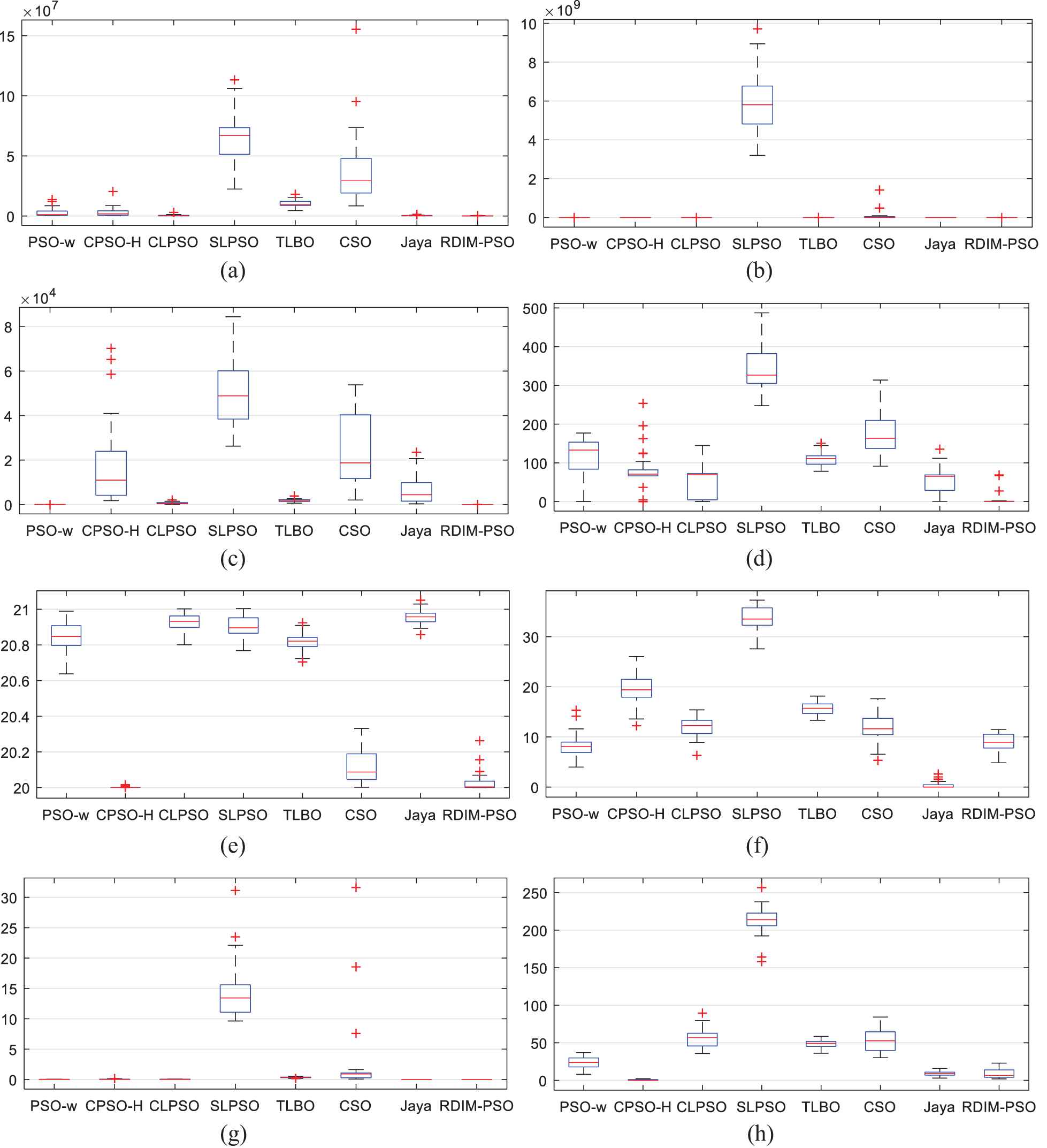

Box-plot of function error values derived from PSO-w, CPSO-H, CLPSO, SLPSO, TLBO, CSO, Jaya and RDIM-PSO on 16 test problems with D = 30. (a) f1; (b) f2; (c) f3; (d) f4; (e) f5; (f) f6; (g) f7; (h) f8; (i) f9; (j) f10; (k) f11; (l) f12; (m) f13; (n) f14; (o) f15; (p) f16.
| F | PSO-w | CPSO-H | CLPSO | SLPSO | TLBO | CSO | Jaya | RDIM-PSO | |
|---|---|---|---|---|---|---|---|---|---|
| Compare/rank | f4 | −/6 | −/2 | −/4 | −/7 | −/5 | −/3 | −/8 | |
| f5 | −/5 | −/2 | −/4 | −/3 | −/7 | −/8 | −/6 | ||
| f6 | +/2 | −/7 | −/5 | +/3 | −/6 | +/1 | −/8 | ||
| f7 | −/3 | −/4 | −/5 | −/7 | −/6 | +/1 | −/8 | ||
| f8 | −/5 | +/1 | −/4 | −/6 | −/7 | +/2 | −/8 | ||
| f9 | +/2 | −/7 | −/6 | +/3 | +/4 | +/1 | −/8 | ||
| f10 | −/5 | +/1 | +/3 | −/7 | −/6 | +/2 | −/8 | ||
| f11 | ≈/2 | ≈/2 | −/6 | ≈/2 | −/7 | +/1 | −/8 | ||
| f12 | −/5 | +/2 | −/4 | +/1 | −/6 | −/7 | −/8 | ||
| f13 | −/5 | ≈/2 | −/4 | −/7 | −/6 | +/1 | −/8 | ||
| f14 | −/7 | −/5 | −/2 | −/6 | −/4 | −/3 | −/8 | ||
| f15 | −/3 | −/6 | −/4 | −/7 | −/5 | −/2 | −/8 | ||
| f16 | −/5 | ≈/1 | −/3 | −/7 | −/6 | −/4 | −/8 | ||
| −/≈/+ | 10/1/2 | 7/3/3 | 12/0/1 | 9/1/3 | 12/0/1 | 6/0/7 | 13/0/0 | ||
| Avg-rank | 4.23 | 3.23 | 4.15 | 5.08 | 5.77 | 2.77 | 7.85 | 2.31 |
Experimental results of PSO-w, CPSO-H, CLPSO, SLPSO, TLBO, CSO, Jaya and RDIM-PSO on f4–f16 with D = 50.
| F | PSO-w | CPSO-H | CLPSO | SLPSO | TLBO | CSO | Jaya | RDIM-PSO | |
|---|---|---|---|---|---|---|---|---|---|
| Compare/rank | f4 | −/6 | −/4 | −/3 | −/7 | −/5 | −/2 | −/8 | |
| f5 | −/5 | −/2 | −/4 | −/3 | −/6 | −/7 | −/8 | ||
| f6 | −/3 | −/6 | −/4 | −/2 | −/7 | −/1 | −/8 | ||
| f7 | −/4 | −/5 | −/3 | −/7 | −/6 | ≈/1 | −/8 | ||
| f8 | −/5 | +/1 | +/2 | −/6 | −/7 | +/3 | −/8 | ||
| f9 | +/2 | −/6 | ≈/3 | +/1 | ≈/3 | −/7 | −/8 | ||
| f10 | −/5 | +/2 | +/1 | −/6 | −/7 | +/3 | −/8 | ||
| f11 | −/5 | −/4 | −/6 | +/2 | −/7 | +/1 | −/8 | ||
| f12 | −/5 | +/2 | −/4 | +/1 | −/7 | −/8 | −/6 | ||
| f13 | −/7 | +/1 | +/3 | +/4 | ≈/5 | +/2 | −/8 | ||
| f14 | −/4 | −/2 | −/6 | −/7 | −/3 | −/5 | −/8 | ||
| f15 | +/1 | ≈/2 | ≈/2 | −/7 | −/6 | ≈/2 | −/8 | ||
| f16 | −/5 | +/1 | ≈/2 | −/4 | −/7 | −/6 | −/8 | ||
| −/≈/+ | 10/0/3 | 7/1/5 | 6/3/4 | 8/0/5 | 11/2/0 | 6/2/5 | 13/0/0 | ||
| Avg-rank | 4.38 | 2.92 | 3.31 | 4.38 | 5.85 | 3.69 | 7.85 | 2.69 |
Experimental results of PSO-w, CPSO-H, CLPSO, SLPSO, TLBO, CSO, Jaya and RDIM-PSO on f4–f16 with D = 100.
(3) Hybrid problems f17–f22
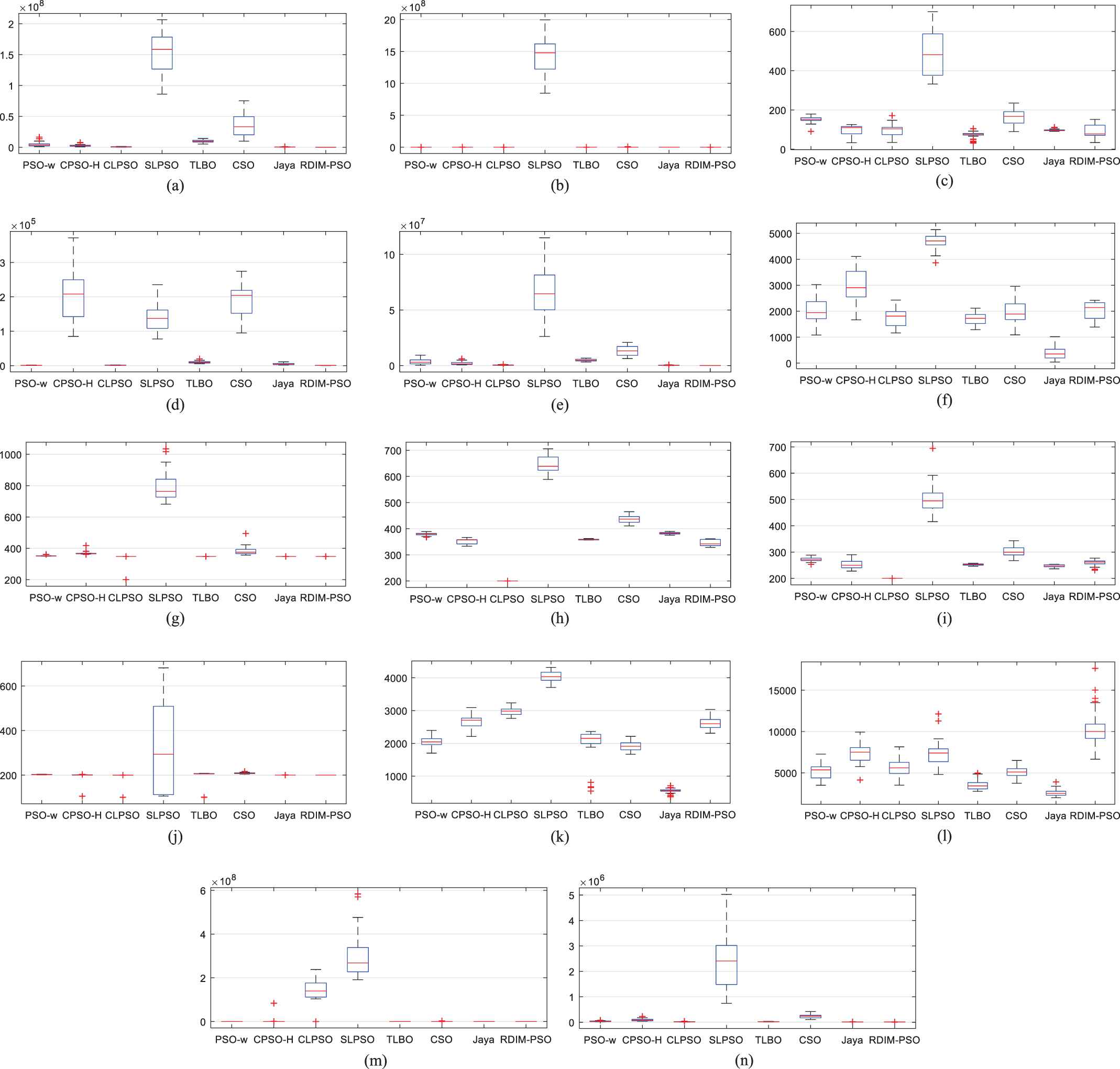
With regard to the hybrid problems f17–f22 when D = 30, the results in Table 7 and Figure 7 show that the proposed RDIM-PSO outperforms other algorithms on f17 and f21. CSO gets the best results on f18, f19 and f22. PSO-w ranks first on f20. RDIM-PSO outperforms PSO-w, CPSO-H, CLPSO, SLPSO, TLBO, CSO and Jaya on 4, 6, 5, 6, 5, 3 and 6 test problems, respectively. The overall Wilcoxon ranking sequences for the test problems are RDIM-PSO, CSO, PSO-w, TLBO, CLPSO, CPSO-H (SLPSO) and Jaya in a descending direction. The average rank of CPSO-H is the same as that of SLPSO. Table 8 shows that RDIM-PSO outperforms PSO-w, CPSO-H, CLPSO, SLPSO, TLBO, CSO and Jaya on 4, 5, 4, 5, 4, 3 and 6 test problems under D = 50, respectively. The overall Wilcoxon ranking sequences for the test problems are RDIM-PSO, CSO, TLBO, PSO-w, CLPSO, CPSO-H, SLPSO and Jaya in a descending direction. Table 9 shows that RDIM-PSO outperforms PSO-w, CPSO-H, CLPSO, SLPSO, TLBO, CSO and Jaya on 5, 5, 3, 5, 3, 3 and 6 test problems under D = 100, respectively. The overall Wilcoxon ranking sequences for the test problems are RDIM-PSO, CSO, TLBO, CLPSO, PSO-w, CPSO-H, SLPSO and Jaya in a descending direction.
| F | PSO-w | CPSO-H | CLPSO | SLPSO | TLBO | CSO | Jaya | RDIM-PSO | |
|---|---|---|---|---|---|---|---|---|---|
| Compare/rank | f17 | −/4 | −/6 | −/5 | −/7 | −/3 | −/2 | −/8 | |
| f18 | −/6 | −/7 | −/3 | −/5 | −/4 | +/1 | −/8 | ||
| f19 | −/3 | −/6 | −/4 | −/7 | −/5 | +/1 | −/8 | ||
| f20 | ≈/1 | −/7 | −/4 | −/8 | −/3 | −/6 | −/5 | ||
| f21 | −/2 | −/6 | −/4 | −/7 | −/3 | −/5 | −/8 | ||
| f22 | +/4 | −/8 | +/2 | −/6 | +/3 | +/1 | −/7 | ||
| −/≈/+ | 4/1/1 | 6/0/0 | 5/0/1 | 6/0/0 | 5/0/1 | 3/0/3 | 6/0/0 | ||
| Avg-rank | 3.33 | 6.67 | 3.67 | 6.67 | 3.50 | 2.67 | 7.33 | 2.00 |
Experimental results of PSO-w, CPSO-H, CLPSO, SLPSO, TLBO, CSO, Jaya and RDIM-PSO on f17–f22 with D = 30.
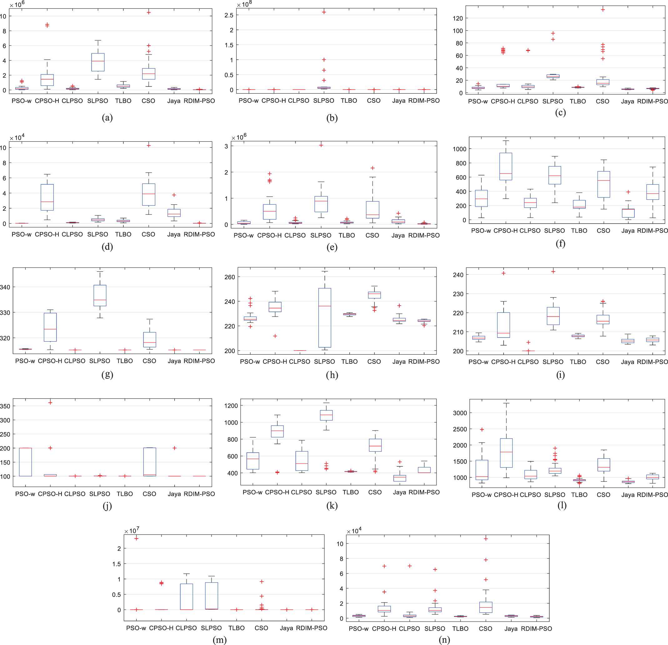
Box-plot of function error values derived from PSO-w, CPSO-H, CLPSO, SLPSO, TLBO, CSO, Jaya and RDIM-PSO on 14 test problems with D = 30. (a) f17; (b) f18; (c) f19; (d) f20; (e) f21; (f) f22; (g) f23; (h) f24; (i) f25; (j) f26; (k) f27; (l) f28; (m) f29; (n) f30.
| F | PSO-w | CPSO-H | CLPSO | SLPSO | TLBO | CSO | Jaya | RDIM-PSO | |
|---|---|---|---|---|---|---|---|---|---|
| Compare/rank | f17 | −/4 | −/5 | −/6 | −/7 | −/3 | −/2 | −/8 | |
| f18 | ≈/1 | ≈/1 | ≈/1 | −/7 | ≈/1 | ≈/1 | −/8 | ||
| f19 | −/6 | −/5 | −/3 | −/7 | −/4 | +/1 | −/8 | ||
| f20 | −/2 | −/8 | −/4 | −/7 | −/3 | −/5 | −/6 | ||
| f21 | −/4 | −/5 | −/6 | −/7 | −/3 | −/2 | −/8 | ||
| f22 | +/4 | −/7 | +/2 | ≈/5 | +/3 | +/1 | −/8 | ||
| −/≈/+ | 4/1/1 | 5/1/0 | 4/1/1 | 5/1/0 | 4/1/1 | 3/1/2 | 6/0/0 | ||
| Avg-rank | 3.50 | 5.17 | 3.67 | 6.67 | 2.83 | 2.00 | 7.67 | 1.83 |
Experimental results of PSO-w, CPSO-H, CLPSO, SLPSO, TLBO, CSO, Jaya and RDIM-PSO on f17–f22 with D = 50.
| F | PSO-w | CPSO-H | CLPSO | SLPSO | TLBO | CSO | Jaya | RDIM-PSO | |
|---|---|---|---|---|---|---|---|---|---|
| Compare/rank | f17 | −/5 | −/4 | −/6 | −/7 | −/3 | −/2 | −/8 | |
| f18 | −/5 | −/6 | +/1 | −/7 | ≈/3 | +/2 | −/8 | ||
| f19 | −/6 | ≈/1 | ≈/1 | −/7 | ≈/1 | ≈/1 | −/8 | ||
| f20 | −/2 | −/8 | −/5 | −/7 | −/3 | −/4 | −/6 | ||
| f21 | −/5 | −/4 | −/6 | −/7 | −/3 | −/2 | −/8 | ||
| f22 | ≈/4 | +/7 | +/2 | ≈/4 | +/3 | +/1 | +/8 | ||
| −/≈/+ | 5/1/0 | 5/1/0 | 3/1/2 | 5/1/0 | 3/2/1 | 3/1/2 | 6/0/0 | ||
| Avg-rank | 4.50 | 5.00 | 3.50 | 6.50 | 2.67 | 2.00 | 7.67 | 1.83 |
Experimental results of PSO-w, CPSO-H, CLPSO, SLPSO, TLBO, CSO, Jaya and RDIM-PSO on f17–f22 with D = 100.
(4) Composite problems f23–f30
Concerning the hybrid problems f23–f30 when D = 30, Table 10 and Figure 7 present that PSO-w, CLPSO, TLBO, CSO and RDIM-PSO achieve similar results on f23. CLPSO, TLBO, Jaya and RDIM-PSO achieve similar results on f26. TLBO ranks first on f24 and f25. CSO is the winner on f27 and f28. RDIM-PSO surpasses all other algorithms on f29 and f30. RDIM-PSO performs better than PSO-w, CPSO-H, CLPSO, SLPSO, TLBO, CSO and Jaya on 8, 8, 5, 8, 5, 3 and 8 test problems, respectively. The overall Wilcoxon ranking sequences for the test problems are RDIM-PSO, CSO, CLPSO, TLBO, PSO-w, SLPSO and CPSO-H (Jaya) in a descending direction. The average rank of CPSO-H is the same as that of Jaya. Table 11 shows that RDIM-PSO performs better than PSO-w, CPSO-H, CLPSO, SLPSO, TLBO, CSO and Jaya on 4, 5, 2, 6, 4, 2 and 7 test problems under D = 50, respectively. The overall Wilcoxon ranking sequences for the test problems are CLPSO (CSO), TLBO (RDIM-PSO), PSO-w (CPSO-H), SLPSO and Jaya in a descending direction. The average rank of CLPSO is the same as that of CSO. The average rank of TLBO is the same as that of RDIM-PSO. The average rank of PSO-w is the same as that of CPSO-H. Table 12 shows that RDIM-PSO performs better than PSO-w, CPSO-H, CLPSO, SLPSO, TLBO, CSO and Jaya on 6, 5, 4, 6, 3, 5 and 7 test problems under D = 100, respectively. The overall Wilcoxon ranking sequences for the test problems are CSO, CLPSO, RDIM-PSO, TLBO, CPSO-H, PSO-w, SLPSO and Jaya in a descending direction.
| F | PSO-w | CPSO-H | CLPSO | SLPSO | TLBO | CSO | Jaya | RDIM-PSO | |
|---|---|---|---|---|---|---|---|---|---|
| Compare/rank | f23 | −/5 | −/7 | −/4 | −/6 | ≈/1 | ≈/1 | −/8 | |
| f24 | −/4 | −/7 | −/5 | −/8 | +/1 | ≈/2 | −/6 | ||
| f25 | −/4 | −/6 | −/5 | −/7 | +/1 | ≈/2 | −/8 | ||
| f26 | −/8 | −/6 | −/3 | −/7 | −/2 | −/5 | −/4 | ||
| f27 | −/5 | −/7 | +/2 | −/6 | −/4 | +/1 | −/8 | ||
| f28 | −/5 | −/8 | +/2 | −/7 | −/4 | +/1 | −/6 | ||
| f29 | −/5 | −/6 | −/2 | −/4 | −/7 | −/3 | −/8 | ||
| f30 | −/4 | −/7 | ≈/1 | −/8 | −/5 | −/3 | −/6 | ||
| −/≈/+ | 8/0/0 | 8/0/0 | 5/1/2 | 8/0/0 | 5/1/2 | 3/3/2 | 8/0/0 | ||
| Avg-rank | 5.00 | 6.75 | 3.00 | 6.63 | 3.13 | 2.25 | 6.75 | 1.75 |
Experimental results of PSO-w, CPSO-H, CLPSO, SLPSO, TLBO, CSO, Jaya and RDIM-PSO on f23–f30 with D = 30.
| F | PSO-w | CPSO-H | CLPSO | SLPSO | TLBO | CSO | Jaya | RDIM-PSO | |
|---|---|---|---|---|---|---|---|---|---|
| Compare/rank | f23 | −/5 | −/6 | −/4 | −/7 | −/3 | ≈/1 | −/8 | |
| f24 | ≈/3 | ≈/3 | +/2 | −/7 | +/1 | ≈/3 | −/8 | ||
| f25 | +/5 | +/3 | +/4 | −/7 | +/1 | +/2 | −/8 | ||
| f26 | −/7 | −/4 | ≈/1 | −/8 | ≈/1 | −/5 | −/6 | ||
| f27 | +/3 | −/7 | +/2 | +/4 | −/6 | +/1 | −/8 | ||
| f28 | +/5 | ≈/7 | +/2 | +/6 | +/3 | +/1 | +/4 | ||
| f29 | −/6 | −/5 | −/2 | −/4 | −/7 | −/3 | −/8 | ||
| f30 | −/6 | −/5 | +/1 | −/7 | −/4 | ≈/2 | −/8 | ||
| −/≈/+ | 4/1/3 | 5/2/1 | 2/1/5 | 6/0/2 | 4/1/3 | 2/3/3 | 7/0/1 | ||
| Avg-rank | 5.00 | 5.00 | 2.25 | 6.25 | 3.25 | 2.25 | 7.25 | 3.25 |
Experimental results of PSO-w, CPSO-H, CLPSO, SLPSO, TLBO, CSO, Jaya and RDIM-PSO on f23–f30 with D = 50.
| F | PSO-w | CPSO-H | CLPSO | SLPSO | TLBO | CSO | Jaya | RDIM-PSO | |
|---|---|---|---|---|---|---|---|---|---|
| Compare/rank | f23 | −/5 | −/6 | −/4 | −/7 | +/1 | −/3 | −/8 | |
| f24 | −/5 | −/3 | −/4 | −/7 | +/1 | −/6 | −/8 | ||
| f25 | −/6 | ≈/4 | +/3 | −/7 | +/1 | +/2 | −/8 | ||
| f26 | −/6 | +/1 | +/2 | −/7 | +/3 | −/5 | −/8 | ||
| f27 | +/4 | −/6 | +/3 | +/2 | −/7 | +/1 | −/8 | ||
| f28 | +/4 | +/6 | +/2 | +/3 | +/5 | +/1 | +/7 | ||
| f29 | −/4 | −/6 | −/3 | −/5 | −/7 | −/2 | −/8 | ||
| f30 | −/5 | −/6 | −/4 | −/7 | −/3 | −/2 | −/8 | ||
| −/≈/+ | 6/0/2 | 5/1/2 | 4/0/4 | 6/0/2 | 3/0/5 | 5/0/3 | 7/0/1 | ||
| Avg-rank | 4.88 | 4.75 | 3.13 | 5.63 | 3.50 | 2.75 | 7.88 | 3.38 |
Experimental results of PSO-w, CPSO-H, CLPSO, SLPSO, TLBO, CSO, Jaya and RDIM-PSO on f23–f30 with D = 100.
Overall, compared with these seven popular optimization algorithms when D = 30, the results based on Wilcoxon's rank-sum test in Table 13 shows the proposed RDIM-PSO is the winner in most cases. Compared with PSO-w, TLBO, SLPSO and Jaya, RDIM-PSO wins on 23, 25, 29 and 30 problems, respectively. Compared with CPSO-H and CLPSO, RDIM-PSO wins on 26 problems. Compared with CSO, RDIM-PSO wins on 14 problems and loses on 11 problems. The overall Wilcoxon ranking sequences for the test problems are RDIM-PSO, CSO, PSO-w, TLBO, CLPSO, CPSO-H, SLPSO and Jaya in a descending direction. RDIM-PSO performs better than PSO-w, CPSO-H, CLPSO, SLPSO, TLBO, CSO and Jaya on 21, 20, 21, 23, 23, 14 and 29 test problems under D = 50, respectively. The overall Wilcoxon ranking sequences for the test problems are RDIM-PSO, CSO, CLPSO, PSO-w (TLBO), CPSO-H, SLPSO and Jaya in a descending direction. The average rank of PSO-w is the same as that of TLBO. RDIM-PSO performs better than PSO-w, CPSO-H, CLPSO, SLPSO, TLBO, CSO and Jaya on 23, 19, 15, 22, 19, 16 and 29 test problems under D = 100, respectively. The overall Wilcoxon ranking sequences for the test problems are RDIM-PSO, CSO, CLPSO, CPSO-H, TLBO, PSO-w, SLPSO and Jaya in a descending direction.
| D | PSO-w | CPSO-H | CLPSO | SLPSO | TLBO | CSO | Jaya | RDIM-PSO | |
|---|---|---|---|---|---|---|---|---|---|
| 30 | −/≈/+ | 23/6/1 | 26/0/4 | 26/1/3 | 29/0/1 | 25/2/3 | 14/5/11 | 30/0/0 | |
| Avg-rank | 3.77 | 5.33 | 4.27 | 6.27 | 4.03 | 2.63 | 7.40 | 1.77 | |
| 50 | −/≈/+ | 21/3/6 | 20/6/4 | 21/2/7 | 23/2/5 | 23/2/5 | 14/4/12 | 29/0/1 | |
| Avg-rank | 4.23 | 4.27 | 3.67 | 5.90 | 4.23 | 2.50 | 7.67 | 2.33 | |
| 100 | −/≈/+ | 23/2/5 | 19/4/7 | 15/5/10 | 22/1/7 | 19/5/6 | 16/4/10 | 29/0/1 | |
| Avg-rank | 4.37 | 3.90 | 3.33 | 5.40 | 4.23 | 3.00 | 7.83 | 2.53 |
Comparison of RDIM-PSO with PSO-w, CPSO-H, CLPSO, SLPSO, TLBO, CSO and Jaya on the CEC2014 benchmark problems (D = 30, D = 50 and D = 100 dimensions).
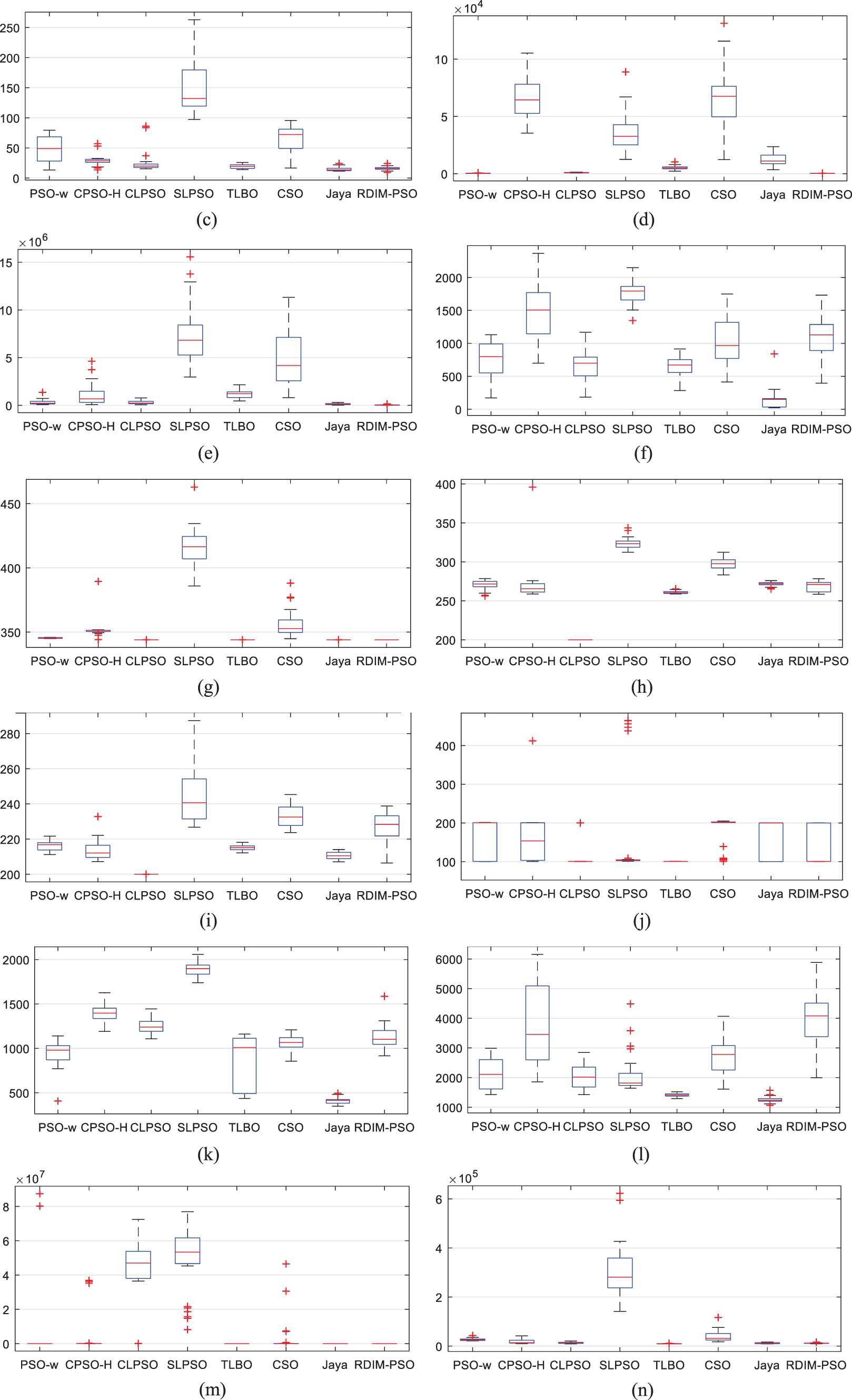
Figures 6–11 show the Box-plot of function error values derived from PSO-w, CPSO-H, CLPSO, SLPSO, TLBO, CSO, Jaya and RDIM-PSO on 30 test problems with D = 30, D = 50 and D = 100, respectively. Generally, the global search and local search abilities always contradict each other. The performance of optimization algorithm relies heavily on the good balance between exploration and exploitation. In the early stage, more exploration is beneficial, while more exploitation is beneficial in the later stage. The proposed RDIM-PSO considers both fitness and diversity information during the optimization process, where the fitness is related to exploitation and the diversity is associated with exploration. In addition, the particles are attracted to different regions (neighborhoods) by the reference directions, which allow more promising neighborhoods to be more intensively searched. Finally, the promising particles are generated by the Gaussian process-based inverse model, which can further improve the performance of RDIM-PSO.
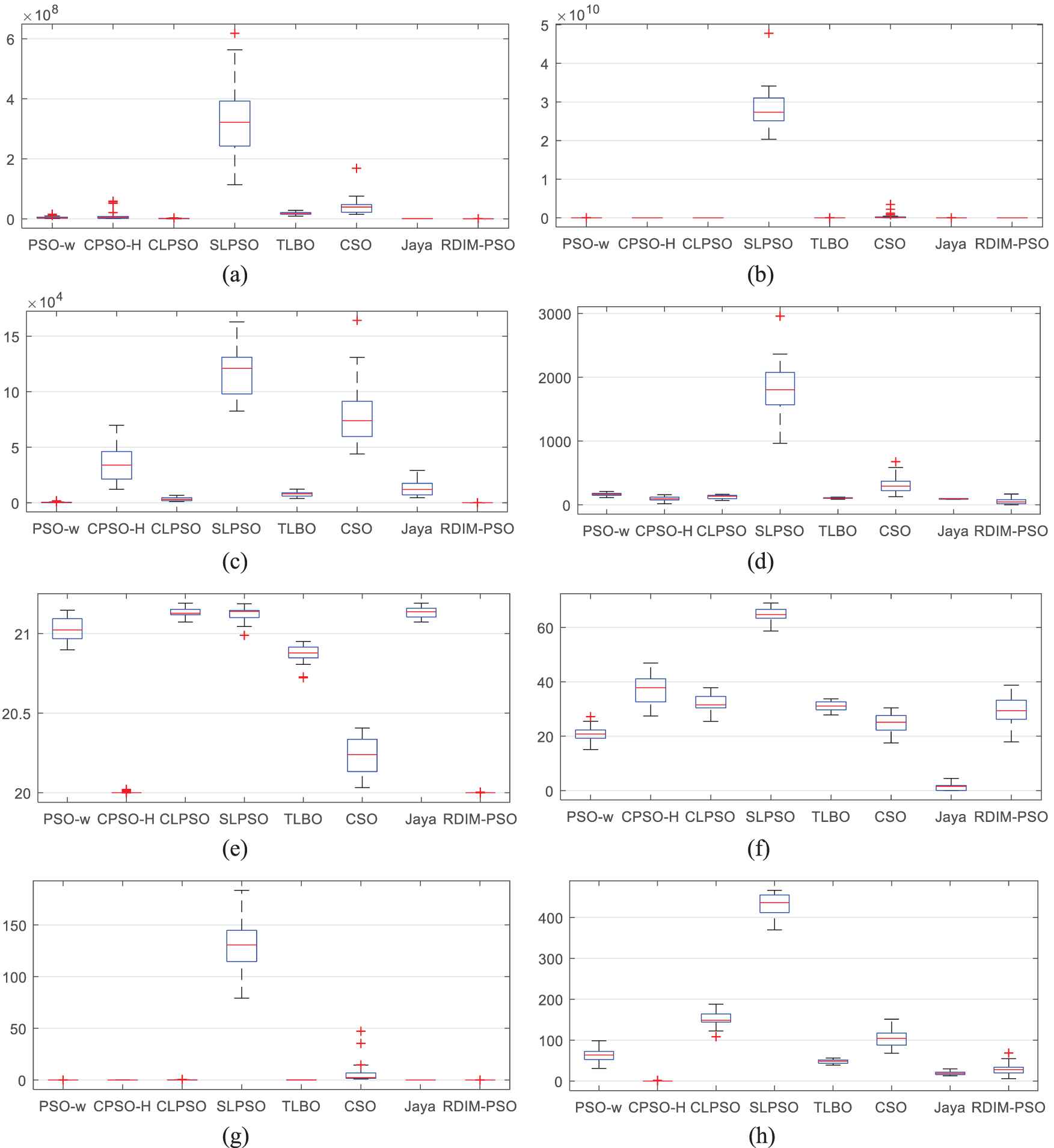

Box-plot of function error values derived from PSO-w, CPSO-H, CLPSO, SLPSO, TLBO, CSO, Jaya and RDIM-PSO on 16 test problems with D = 50. (a) f1; (b) f2; (c) f3; (d) f4; (e) f5; (f) f6; (g) f7; (h) f8; (i) f9; (j) f10; (k) f11; (l) f12; (m) f13; (n) f14; (o) f15; (p) f16.

Box-plot of function error values derived from PSO-w, CPSO-H, CLPSO, SLPSO, TLBO, CSO, Jaya and RDIM-PSO on 14 test problems with D = 50. (a) f17; (b) f18; (c) f19; (d) f20; (e) f21; (f) f22; (g) f23; (h) f24; (i) f25; (j) f26; (k) f27; (l) f28; (m) f29; (n) f30.
Box-plot of function error values derived from PSO-w, CPSO-H, CLPSO, SLPSO, TLBO, CSO, Jaya and RDIM-PSO on 16 test problems with D = 100. (a) f1; (b) f2; (c) f3; (d) f4; (e) f5; (f) f6; (g) f7; (h) f8; (i) f9; (j) f10; (k) f11; (l) f12; (m) f13; (n) f14; (o) f15; (p) f16.
Box-plot of function error values derived from PSO-w, CPSO-H, CLPSO, SLPSO, TLBO, CSO, Jaya and RDIM-PSO on 14 test problems with D = 100. (a) f17; (b) f18; (c) f19; (d) f20; (e) f21; (f) f22; (g) f23; (h) f24; (i) f25; (j) f26; (k) f27; (l) f28; (m) f29; (n) f30.
In order to test the statistical significance of the eight compared algorithms, the Wilcoxon's test at the 5% significance level, which is implemented by using KEEL software [49], is employed based on the PR values. Tables 14–19 summarizes the statistical test results. It can be seen from Tables 14, 16, and 18 that RDIM-PSO provides higher R+ values than R− values compared with PSO-w, CPSO-H, CLPSO, SLPSO, TLBO, CSO and Jaya. Furthermore, the p values of PSO-w, CPSO-H, SLPSO, TLBO and Jaya are less than 0.05, which means that RDIM-PSO is significantly better than these competitors. The p values of CSO is greater than 0.05, which means that the performance of RDIM-PSO is not different from that of CSO. Similarly, the p values of CLPSO is greater than 0.05 when D = 50 and D = 100, which means that the performance of CLPSO is not different from that of CSO. To further determine the ranking of the eight compared algorithms, the Friedman's test, which is also implemented by using KEEL software, is conducted. As shown in Table 15, the overall ranking sequences for the test problems are RDIM-PSO, CSO, PSO-w, TLBO, CLPSO, CPSO-H, SLPSO and Jaya. Table 17 shows the overall ranking sequences for the test problems are RDIM-PSO, CSO, CLPSO, TLBO, PSO-w, CPSO-H, SLPSO and Jaya. Table 19 shows the overall ranking sequences for the test problems are RDIM-PSO, CSO, CLPSO, CPSO-H, TLBO, PSO-w, SLPSO and Jaya. Therefore, it can be concluded that the improvement strategies are effective.
| VS | R+ | R– | Exact p-Value | Asymptotic p-Value |
|---|---|---|---|---|
| PSO-w | 390.0 | 45.0 | ≥0.2 | 0.000183 |
| CPSO-H | 404.0 | 31.0 | ≥0.2 | 0.00005 |
| CLPSO | 411.5 | 53.5 | ≥0.2 | 0.000222 |
| SLPSO | 462.0 | 3.0 | ≥0.2 | 0.000002 |
| TLBO | 417.5 | 47.5 | ≥0.2 | 0.000131 |
| CSO | 278.0 | 187.0 | ≥0.2 | 0.344075 |
| Jaya | 435.0 | 0.0 | ≥0.2 | 0.000002 |
Results obtained by the Wilcoxon test for algorithm RDIM-PSO with D = 30.
| Algorithm | Ranking |
|---|---|
| RDIM-PSO | 2.0167 |
| PSO-w | 3.7667 |
| CPSO-H | 5.3667 |
| CLPSO | 4.2833 |
| SLPSO | 6.2667 |
| TLBO | 4.15 |
| CSO | 2.75 |
| Jaya | 7.4 |
Average ranking of the algorithms (Friedman) with D = 30.
| VS | R+ | R– | Exact p-Value | Asymptotic p-Value |
|---|---|---|---|---|
| PSO-w | 361.0 | 104.0 | ≥0.2 | 0.00781 |
| CPSO-H | 392.5 | 72.5 | ≥0.2 | 0.000963 |
| CLPSO | 284.0 | 151.0 | ≥0.2 | 0.147406 |
| SLPSO | 377.0 | 88.0 | ≥0.2 | 0.00286 |
| TLBO | 352.0 | 83.0 | ≥0.2 | 0.00351 |
| CSO | 264.0 | 171.0 | ≥0.2 | 0.309491 |
| Jaya | 447.0 | 18.0 | ≥0.2 | 0.00001 |
Results obtained by the Wilcoxon test for algorithm RDIM-PSO with D = 50.
| Algorithm | Ranking |
|---|---|
| RDIM-PSO | 2.65 |
| PSO-w | 4.4833 |
| CPSO-H | 4.5667 |
| CLPSO | 3.6167 |
| SLPSO | 5.9 |
| TLBO | 4.3833 |
| CSO | 2.7 |
| Jaya | 7.7 |
Average ranking of the algorithms (Friedman) with D = 50.
| VS | R+ | R– | Exact p-Value | Asymptotic p-Value |
|---|---|---|---|---|
| PSO-w | 366.5 | 98.5 | ≥0.2 | 0.005544 |
| CPSO-H | 332.0 | 103.0 | ≥0.2 | 0.012895 |
| CLPSO | 238.0 | 197.0 | ≥0.2 | 0.649766 |
| SLPSO | 371.0 | 94.0 | ≥0.2 | 0.00425 |
| TLBO | 333.5 | 131.5 | ≥0.2 | 0.036343 |
| CSO | 238.5 | 196.5 | ≥0.2 | 0.642004 |
| Jaya | 448.0 | 17.0 | ≥0.2 | 0.000009 |
Results obtained by the Wilcoxon test for algorithm RDIM-PSO with D = 100.
| Algorithm | Ranking |
|---|---|
| RDIM-PSO | 3.0833 |
| PSO-w | 4.5667 |
| CPSO-H | 4.1833 |
| CLPSO | 3.3833 |
| SLPSO | 5.4 |
| TLBO | 4.4167 |
| CSO | 3.1667 |
| Jaya | 7.8 |
Average ranking of the algorithms (Friedman) with D = 100.
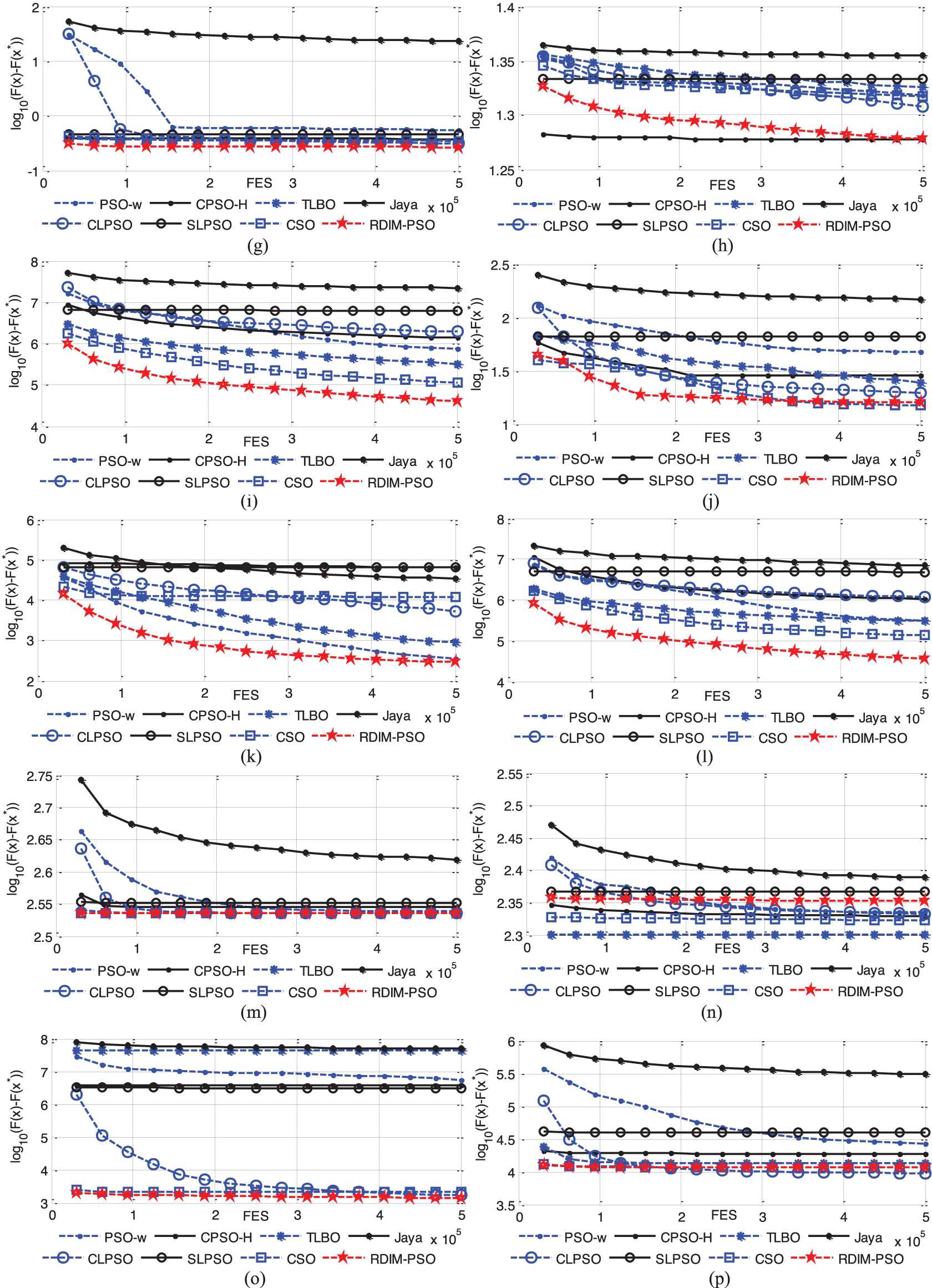
To illustrate the convergence speed of the proposed RDIM-PSO, the convergence curves on 30-dimensional, 50-dimensional and 100-dimensional CEC2014 benchmark problems are presented in Figures 12–14, respectively. There are 16 representative problems including 2 unimodal problems, 6 multimodal problems, 4 hybrid problems and 4 composite problems. The curves illustrate mean errors (in logarithmic scale) in 30 independent simulations of PSO-w, CPSO-H, CLPSO, SLPSO, TLBO, CSO, Jaya and RDIM-PSO. As mentioned above, the curves indicate that, in most problems, RDIM-PSO either achieves a fast convergence or behaves similarly to it.
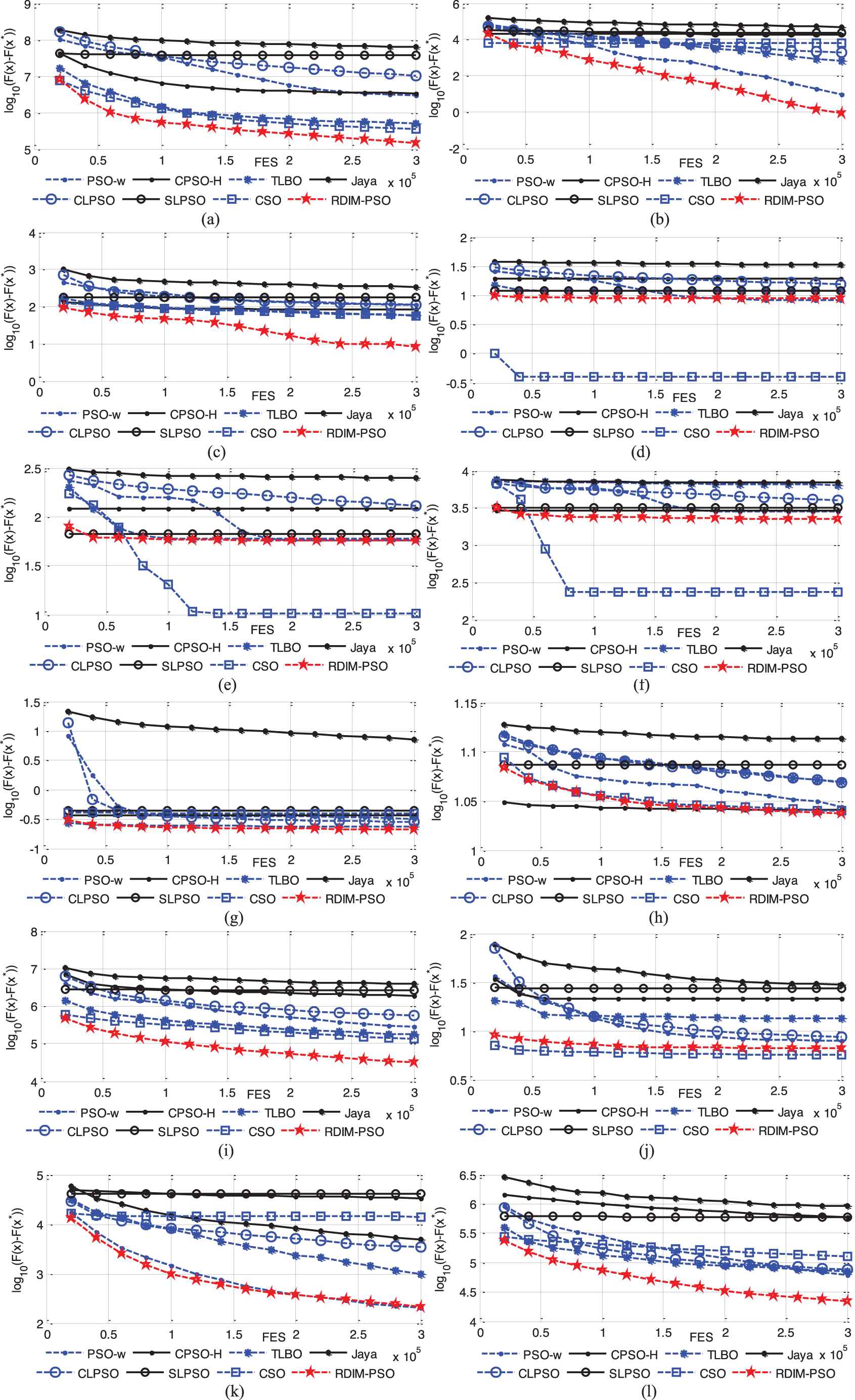
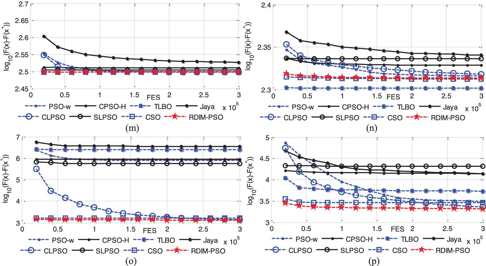
Evolution of the mean function error values derived from PSO-w, CPSO-H, CLPSO, SLPSO, TLBO, CSO, Jaya and RDIM-PSO versus the number of FES on 16 test problems with D = 30. (a) f1; (b) f3; (c) f4; (d) f6; (e) f9; (f) f11; (g) f14; (h) f16; (i) f17; (j) f19; (k) f20; (l) f21; (m) f23; (n) f25; (o) f29; (p) f30.

Evolution of the mean function error values derived from PSO-w, CPSO-H, CLPSO, SLPSO, TLBO, CSO, Jaya and RDIM-PSO versus the number of FES on 16 test problems with D = 50. (a) f1; (b) f3; (c) f4; (d) f6; (e) f9; (f) f11; (g) f14; (h) f16; (i) f17; (j) f19; (k) f20; (l) f21; (m) f23; (n) f25; (o) f29; (p) f30.


Evolution of the mean function error values derived from PSO-w, CPSO-H, CLPSO, SLPSO, TLBO, CSO, Jaya and RDIM-PSO versus the number of FES on 16 test problems with D = 100. (a) f1; (b) f3; (c) f4; (d) f6; (e) f9; (f) f11; (g) f14; (h) f16; (i) f17; (j) f19; (k) f20; (l) f21; (m) f23; (n) f25; (o) f29; (p) f30.
5. THE REAL-WORLD OPTIMIZATION PROBLEM
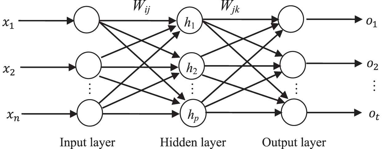
To test the performance of the proposed RDIM-PSO algorithm on solving the real-world problem, time series prediction with the ANN is chosen as the testing objective. The ANN is fit for solving the problems of chaotic time series prediction and functions approximation. It is an effective way that verify the effectiveness of algorithm by training the parameters of ANN. Various heuristic optimization algorithms have been used to do this, such as PSO [50], DE [51], GAs [52], Ant colony algorithm [53], hybrid particle swarm optimization and gravitational search algorithm (PSOGSA) [54], etc. To deeply verify the effectiveness of the RDIM-PSO, a three-layer feed-forward network which includes input units, hidden units and output units is selected for chaotic time series prediction and function approximation. The three-layer ANN is depicted in Figure 15.
Structure of a three-layer feed forward neural network.
In Figure 15, X = (x1, x2, …, xi, …xn)T is input layer, O = (o1, o2, …, ok, …ot)T is output layer. Wij and Wjk is the weight between the I–H (input layer and hidden layer) and H–O (hidden layer and output layer), respectively. i = 1, 2, …, n. j = 1, 2, …, p, k = 1, 2, …, t. The aim of neural network training is to find a set of weights with the smallest error measure. Therefore, the mean sum of squared errors (MSE) is selected as an evaluation indicator of optimization algorithms, shown as follows:
5.1. SISO Nonlinear Function Approximation
In this example, there are one input units, five hidden units and one output units in the three-layer feed-forward ANN. The SISO nonlinear system used in this experiment is given as follows [55]:
In this experiment, the number (dimension) of the variables is 16. Moreover, 200 pairs of data are chosen from Eq. (19) as the training samples. Eight optimization algorithms are used to optimize the neural network. NP (population size) = 50; FES (maximal number of function evaluations) = 10,000. The other parameters of the different algorithms are the same as those used in CEC2014. Experiments introduce 30db additive with Gaussian noise to assess the performance of each algorithm in noise. For each algorithm, 30 independent runs are performed. Here, “Mean” (average best value of the MSE) and “Std” (standard deviation of MSE) are used as evaluation indicators.
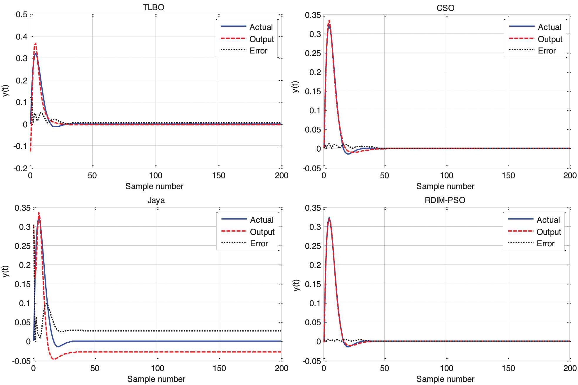
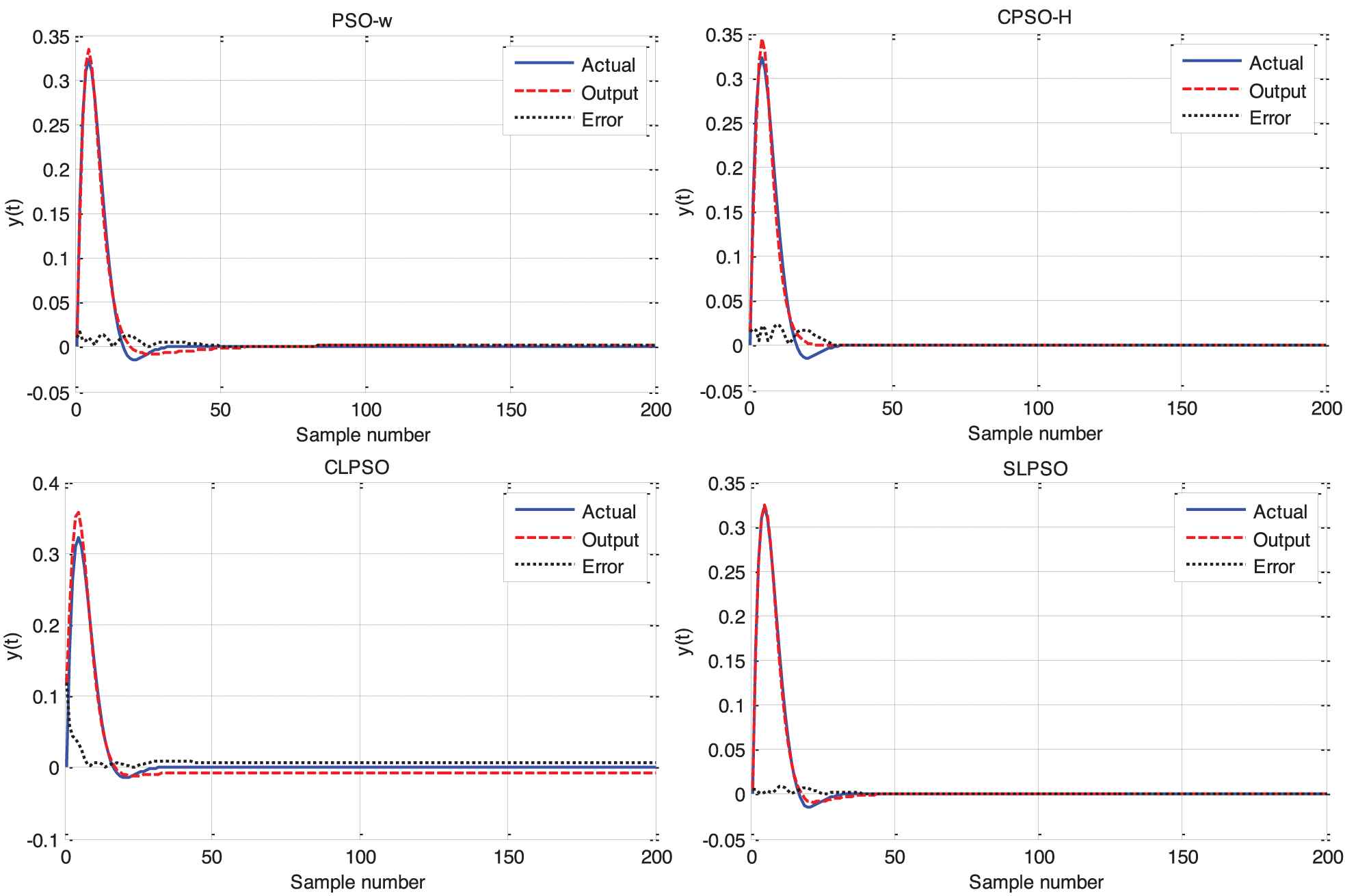
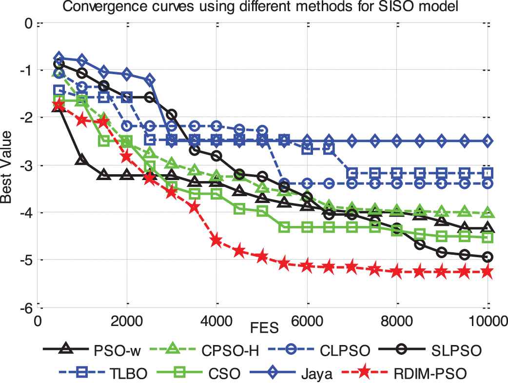
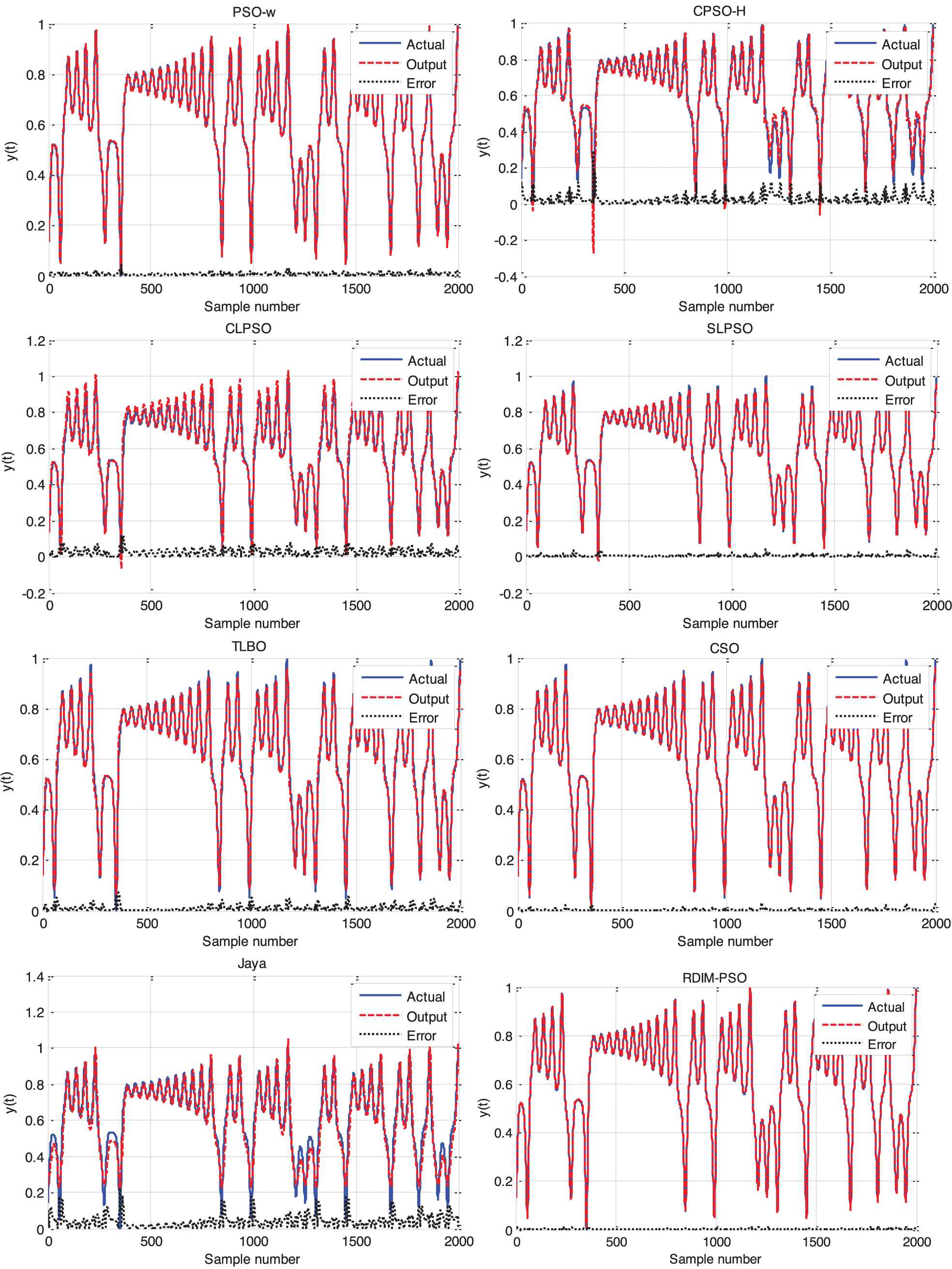
Table 20 shows that mean MSE of RDIM-PSO is the smallest, and the Testing Error Std of RDIM-PSO is the smallest of the eight algorithms. In the case of Training Error Std, SLPSO performs best and RDIM-PSO ranks second. To show the modeling effectiveness of different optimization algorithms, the modeling curves for training and test are shown in Figure 16, and the absolute errors are also displayed in the corresponding curves for the algorithms. Figure 16 indicates that RDIM-PSO outperforms other algorithms for the testing error of ANN. The convergence process according to FES is shown in Figure 17, which shows that the convergence speed of RDIM-PSO is faster than that of the other algorithms.
| Algorithm | Training Error |
Testing Error |
||
|---|---|---|---|---|
| Mean | Std | Mean | Std | |
| PSO-w | 2.0497e-004 | 1.3639e-004 | 6.2057e-003 | 3.1014e-002 |
| CPSO-H | 9.8596e-004 | 1.0796e-003 | 2.9835e-002 | 6.2301e-002 |
| CLPSO | 5.9241e-003 | 4.5272e-003 | 3.4094e-003 | 2.9087e-003 |
| SLPSO | 6.8686e-005 | 2.9278e-005 | 7.9149e-005 | 2.5779e-004 |
| TLBO | 3.7084e-003 | 2.1537e-003 | 3.2755e-003 | 7.3220e-003 |
| CSO | 1.0683e-004 | 5.5269e-005 | 1.6601e-004 | 4.9784e-004 |
| Jaya | 1.5481e-002 | 1.0563e-002 | 8.4399e-003 | 6.8823e-003 |
| RDIM-PSO | 4.5627e-005 | 3.0486e-005 | 6.8852e-005 | 2.2011e-004 |
Comparisons between PSO-w, CPSO-H, CLPSO, SLPSO, TLBO, CSO, Jaya and RDIM-PSO on MSE.
The model and absolute error of different algorithms for SISO system.
The average fitness curves of eight algorithms for SISO system.
5.2. Lorenz Chaotic Time Series Prediction
The Lorenz chaotic system [56] is described as follows:
Our task of this study is to use the earlier three points x(t − 6), x(t − 3) and x(t) to predict the next point x(t + 1). The goal of this experiment is to build the single-step-ahead prediction model of chaotic time series of Lorenz, shown as follows [56]:
To predict the Lorenz model, there are three input units, five hidden units and one output units in the three-layer feed-forward ANN. Like the experiment of Section 5.1, NP = 50, FES = 10,000. The 10,000 data are selected from the model, in which the first 8000 data are discarded. The rest 2000 data are normalized and divided into two groups. One group has 1500 points which act as the training samples, and the other group has 500 points which act as the testing samples. MSE is chosen as the fitness function of all algorithms. The merits in terms of Mean and Std of the training and testing process are shown in Table 21. These results come from 30 independent runs of each of the eight algorithms.
| Algorithm | Training Error |
Testing Error |
||
|---|---|---|---|---|
| Mean | Std | Mean | Std | |
| PSO-w | 4.5861e-004 | 3.4699e-004 | 4.7360e-004 | 3.6247e-004 |
| CPSO-H | 1.2946e-002 | 1.8885e-002 | 1.3313e-002 | 1.8970e-002 |
| CLPSO | 5.2244e-003 | 2.1412e-003 | 5.3556e-003 | 2.1398e-003 |
| SLPSO | 2.8744e-004 | 2.6103e-004 | 3.0806e-004 | 2.7996e-004 |
| TLBO | 5.0261e-003 | 3.0655e-003 | 5.1453e-003 | 3.1560e-003 |
| CSO | 1.9086e-004 | 1.5304e-004 | 2.0688e-004 | 1.6889e-004 |
| Jaya | 1.3970e-002 | 6.4265e-003 | 1.4490e-002 | 6.8396e-003 |
| RDIM-PSO | 1.6213e-004 | 1.7993e-004 | 1.6839e-004 | 1.8640e-004 |
Comparisons between PSO-w, CPSO-H, CLPSO, SLPSO, TLBO, CSO, Jaya and RDIM-PSO on MSE.
Table 21 shows that RDIM-PSO outperformed the other algorithms. The mean deviation of the training error and testing error obtained by RDIM-PSO is ranked first of the eight algorithms. Concerning the standard deviation of the training error and testing error, CSO performs best and RDIM-PSO ranks second. The training and testing curves for 2000 samples are shown in Figure 18. The convergence process of the average MSE for all algorithms is displayed in Figure 19. The figure shows that the convergence speed of RDIM-PSO is faster than that of the other algorithms for Lorenz system. The experimental results indicate that the approximate accuracy of RDIM-PSO is high.
The model and absolute error of different algorithms for Lorenz system.

The average fitness curves of eight algorithms for Lorenz system.
5.3. Box–Jenkins Chaotic Time Series
The third problem is the Box–Jenkins gas furnace (Box–Jenkins) prediction. The Box–Jenkins gas furnace dataset was recorded from a combustion process of a methane–air mixture. There are originally 296 data points (x(t), u(t)), from t = 1 to t = 296. x(t) is the output CO2 concentration and u(t) is the input gas flowing rate.
Our task of this study is to use the earlier points u(t − 4) and x(t − 1) to predict the value of the time series at the point x(t + 1). Our experimental aim is to build the single-step-ahead prediction model of chaotic time series, shown as followings [57,58]:
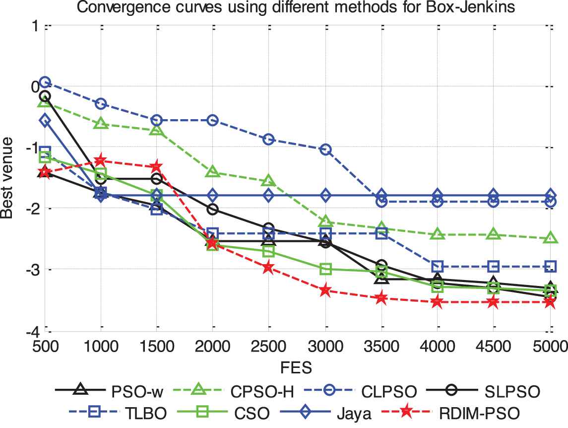
To predict the Box–Jenkins model, there are two input units, five hidden units and one output units in the three-layer feed-forward ANN. 292 data pairs are selected from the real model. The data are divided into two groups. One group has 142 data pairs which act as the training samples. The other group has 150 data pairs which act as the testing samples. Like the experiment of Section 5.1, NP = 50, FES = 5000. The merits in terms of the mean optimum solution (Mean) and the standard deviation of the solutions (Std) in the training and testing process are shown in Table 16. These results come from 30 independent runs of each of the eight algorithms.
From Table 22, it is observed that RDIM-PSO outperformed other seven algorithms in the mean MSE and std MSE in both training and testing cases. Figures 20 and 21 represent the training and testing curves and the convergence process of the average MSE for all algorithms, respectively. The figure shows that the convergence speed of RDIM-PSO is faster than that of the other algorithms for Box–Jenkins system. Then, it can be concluded that RDIM-PSO is the most effective learning algorithm for training the model.
| Algorithm | Training Error |
Testing Error |
||
|---|---|---|---|---|
| Mean | Std | Mean | Std | |
| PSO-w | 2.7440e-003 | 2.6438e-003 | 4.2470e-003 | 3.9781e-003 |
| CPSO-H | 7.9915e-002 | 7.8607e-002 | 1.2020e-001 | 1.1165e-001 |
| CLPSO | 4.3867e-002 | 2.8976e-002 | 4.4900e-002 | 3.0854e-002 |
| SLPSO | 7.8569e-004 | 5.8067e-004 | 1.7505e-003 | 1.4053e-003 |
| TLBO | 3.1100e-003 | 2.2400e-003 | 4.0338e-003 | 2.8770e-003 |
| CSO | 1.2168e-003 | 9.2267e-004 | 2.4789e-003 | 1.2699e-003 |
| Jaya | 1.2345e-001 | 8.9826e-002 | 1.3974e-001 | 1.2677e-001 |
| RDIM-PSO | 6.6152e-004 | 5.0912e-004 | 1.4904e-003 | 1.0095e-003 |
Comparisons between PSO-w, CPSO-H, CLPSO, SLPSO, TLBO, CSO, Jaya and RDIM-PSO on MSE.

The model and absolute error of different algorithms for Box–Jenkins system.
The average fitness curves of eight algorithms for Box–Jenkins system.
6. CONCLUSIONS
This paper presents an enhanced PSO based on reference direction and inverse model. In the proposed algorithm, the reference particles are first selected according to their fitness and diversity contribution with non-dominated sorting. The dynamic neighborhood strategy is employed to divide the population into several sub-swarms with the reference directions. Next, Gaussian process-based inverse model are introduced to generate equilibrium particles by sampling the objective space. Finally, the velocity update strategy is utilized to improve the convergence of the algorithm. Since fitness and diversity information is simultaneously considered to select the best particle in the dynamic neighborhood, a good balance between exploration and exploitation can be ensured. Based on the results of the eight algorithms on CEC2014 test problems and chaotic time series prediction problems, it can be concluded that RDIM-PSO significantly improves the performance of the original PSO algorithm when compared with seven other optimization algorithms.
Future work will extend the application domain of RDIM-PSO, such as Radial basis function networks, Kohonen networks, etc. In addition, we will focus on making full use of the problem landscape information to design a stronger exploration strategy because RDIM-PSO cannot find the global optimum for some composite problems. Finally, RDIM-PSO will be expected to solve the multiobjective optimization problems and constrained optimization problems.
DATA AVAILABILITY STATEMENT
The experimental data used to support the findings of this study are included within the article.
CONFLICT OF INTERESTS
The authors declare they have no conflicts of interest.
AUTHORS' CONTRIBUTIONS
All authors contributed to the work. All authors read and approved the final manuscript.
ACKNOWLEDGMENTS
This research is partly supported by the Doctoral Foundation of Xi'an University of Technology (112-451116017), National Natural Science Foundation of China under Project Code (61803301, 61773314) and the Scientific Research Foundation of the National University of Defense Technology (grant no. ZK18-03-43).
REFERENCES
Cite this article
TY  - JOUR
AU  - Wei Li
AU  - Yaochi Fan
AU  - Qingzheng Xu
PY  - 2020
DA  - 2020/02/03
TI  - Enhanced Particle Swarm Optimization Based on Reference Direction and Inverse Model for Optimization Problems
JO  - International Journal of Computational Intelligence Systems
SP  - 98
EP  - 129
VL  - 13
IS  - 1
SN  - 1875-6883
UR  - https://doi.org/10.2991/ijcis.d.200127.001
DO  - 10.2991/ijcis.d.200127.001
ID  - Li2020
ER  -