
A Multi-Criteria Group Decision-Making Approach Based on Improved BWM and MULTIMOORA with Normal Wiggly Hesitant Fuzzy Information
- DOI
- 10.2991/ijcis.d.200325.001How to use a DOI?
- Keywords
- Multi-criteria group decision-making (MCGDM); Normal wiggly hesitant fuzzy set (NWHFS); Best-worst method (BWM); MULTIMOORA method; Train selection; Spring Festival travel rush
- Abstract
Multi-criteria group decision-making (MCGDM) problems are widespread in real life. However, most existing methods, such as hesitant fuzzy set (HFS), hesitant fuzzy linguistic term set (HFLTS) and inter-valued hesitant fuzzy set (IVHFS) only consider the original evaluation data provided by experts but fail to dig the concealed valuable information. The normal wiggly hesitant fuzzy set (NWHFS) is a useful technique to depict experts’ complex evaluation information toward MCGDM issues. In this paper, on the basis of the score function of NWHFS, we propose the linear best-worst method (BWM)-based weight-determining models with normal wiggly hesitant fuzzy (NWHF) information to compute the optimal weights of experts and criteria. In addition, we present some novel distance measures between NWHFSs and discuss their properties. After fusing the individual evaluation matrices, the NWHF-ranking position method is put forward to develop the group MULTIMOORA method, which can be determined by the final decision results. Moreover, we investigate the Spring Festival travel rush phenomenon deeply and apply our methodology to solve the train selection problem during the Spring Festival period. Finally, the applicability and superiority of the proposed approach is demonstrated by comparing with traditional methods based on two aggregation operators of NWHFSs.
- Copyright
- © 2020 The Authors. Published by Atlantis Press SARL.
- Open Access
- This is an open access article distributed under the CC BY-NC 4.0 license (http://creativecommons.org/licenses/by-nc/4.0/).
1. INTRODUCTION
With the ever-increasing uncertainty in practical decision-making issues, one of the most popular methodology to describe the decision makers (DMs) evaluation information is the idea that using hesitant fuzzy set (HFS) [1,2]. Amounts of scholars devoted themselves to improving the HFS theory and meanwhile got many extensions. Rodríguez et al. [3] put forward the hesitant fuzzy linguistic term set (HFLTS), which is more in line with DMs’ expressions and cognitions. Chen et al. [4] defined the inter-valued hesitant fuzzy set (IVHFS) and then discussed in detail about the aggregation operators of IVHFS. When the membership degrees of hesitant fuzzy element (HFE) cannot be given as several crisp numbers, the triangular fuzzy hesitant fuzzy set (TFHFS) was proposed to remedy the shortcoming [5]. Although these extensions of HFS are widely applied in decision-making problems, we find that the expression forms become more and more complex to depict the whole evaluations of DMs. Besides, Rodríguez et al. [6] summarized the necessity of diverse extensions of HFS and provided the guidance that the extensions of HFS should follow. According to this line, in order to reflect the cognition and hesitation of DMs in real world context more realistic, Ren et al. [7] presented the normal wiggly hesitant fuzzy set (NWHFS), which maintains the original evaluation information in HFEs and dig the potential uncertain information automatically. Lately, Narayanamoorthy et al. [8] extended the NWHFS into the normal wiggly dual hesitant fuzzy sets (NWDHFS). As a matter of fact, the evaluation results will be more convinced by taking both original evaluations and concealed information into account.
Multi-criteria group decision-making (MCGDM) is a complex issue which happens frequently in daily life. Generally, the MCGDM problem can be divided into two types: DMs provide preference relations for pairwise comparisons over a set of alternatives or give their evaluations of alternatives with respect to criteria. The critical factor in dealing with MCGDM problem is to construct a reasonable consensus model. Labella et al. [9] analyzed multiple classical consensus models in large-scale group decision-making (LS-GDM), and Palomares and Martínez [10] designed a new consensus support system. Since the outstanding properties of HFS and its extension forms, many scholars have applied them in MCGDM problems. For instance, Liao et al. [11] introduced multiplicative consistency for hesitant fuzzy preference relations. Rodríguez et al. [12] proposed a novel consensus reaching process to cope with LS-GDM by using HFS. Wu et al. [13] investigated consistency and consensus processes to deal with hesitant fuzzy linguistic preference relations. Besides, Xia et al. [14], Yu et al. [15,16] explored aggregation methods to integrate personal evaluations under the hesitant fuzzy environment. Wang et al. [17] collected all of the evaluation values provided by DMs and produced multi-hesitant fuzzy linguistic term elements. Apart from that, many MCGDM problems were solved by using the ranking methods of HFS and its extension theory. Ahmad et al. [18] employed a hesitant fuzzy VIKOR method for energy project selection. Joshi and Kumar [19] applied TOPSIS in candidates selection problems and Galo et al. [20] presented ELECTRE TRI method combined with HFS in supplier categorization. However, the aforementioned researches did not take the concealed information relates to original evaluation values provided by DMs into account. Ren et al. [7] pointed out that DMs’ cognitive uncertainty can be seen as a normal distribution in a wiggly range centered on an evaluation value. Based on the original possible values in HFE, NWHFS uses the corresponding real preference degree function and wiggly function to reflect the DMs’ concealed attitudinal preferences. Therefore, compared with only considering the original information, tackling MCGDM problems under the normal wiggly hesitant fuzzy (NWHF) environment is more logical and reasonable.
Chen and Hwang believed that the critical step of solving MCGDM problems is to determine the weights of criteria [21]. Lots of work have been done to address the problem of weight-determining. Li et al. [22] focused on solving the MCGDM issues with incomplete weight information by utilizing Shapley function under the hesitant fuzzy environment. Gitinavard et al. [23] derived an extended maximizing deviation method with IVHFS theory to compute the optimal weights of criteria. Joshi et al. [24] constructed an entropy-based weighting model to calculate the criteria weights in the expansion of MCGDM problems. Ren et al. [25] obtained the corresponding weight values by using Analytic Hierarchy Process (AHP). Recently, Rezaei [26] presented a novel technique to do structured pairwise comparisons and determine the weights of criteria, named the best-worst method (BWM). The structured way is to compare the best and worst criteria with all the other criteria, whose times of pairwise comparisons are much less than AHP. Due to the advantages of BWM, it has attracted many scholars’ attention and been widely applied into the MCGDM problems. Hafezalkotob et al. [27,28] determined the expertise degrees and the weights of criteria via the BWM. What’s more, in order to depict the DMs’ evaluations more accurately, the BWM has been integrated with HFS theory. For example, Ali and Rashid [29] described the reference comparison of each criterion with the best and worst criteria by the linguistic terms expressed in HFEs. Mi and Liao [30] deduced a BWM-based weighting model with hesitant fuzzy information. In this paper, we extend the HFS into NWHFS to dig the deeper valuable information and combine it with BWM to derive the weight vectors of expert panel and criteria.
MULTIMOORA is well known as a robust ranking system that consists of three subordinate approaches, namely, the ratio system, the reference point approach and the full multiplicative form. It aggregates ranking results from the triple approaches by employing dominance theory [31]. The MULTIMOORA method has developed by integrating with various fuzzy sets theory [32], especially the HFS and its extension theories. Zeng et al. [33] and Li [34] applied the HFS-MULTIMOORA method to solve MCGDM problems. Liao et al. [35] proposed a new score function of HFLTS and combined with the MULTIMOORA method to derive decision results. Liu et al. [36] put forward a modified MULTIMOORA based on HFLTS and applied it to select the optimal robot. Luo and Li [37] extended the MULTIMOORA to accommodate possibility distribution hesitant fuzzy linguistic term circumstances. Moreover, this method has been utilized in many various real-life applications, such as the risk of failure modes evaluation [38,39], bike-sharing programs assessment [35,40] and vehicle selection [41].
Spring Festival travel rush is a unique traffic phenomenon in China. During the Spring Festival period, a large number of migrant workers and students travel hundreds of thousands of miles to be with their families. The holiday triggers what’s known as the largest annual human migration in the world. More than 400 million travelers chose to take trains during the Spring Festival 2019. Some scholars have focused their attention on the study of Spring Festival travel rush and traffic management. Zuo and Pan [42] investigated the decisive factors for students choosing railway travel. Furthermore, Pan [43] designed a choice experiment to illustrate which factors determine the students’ choice of train trips. Hu [44] investigated the population distribution and population migration center during the Spring Festival, and Yin et al. [45] explored the reverse migration phenomenon and its influences. What’s more, Chen et al. [46] put forward lots of suggestion for the development of Chinese high-speed rail. Sama et al. [47] dealt with the real-time train routing selection problem. In fact, choosing a suitable train to return home during the Spring Festival travel rush is restricted by multiple factors, hence, the train selection problem can be considered as a MCGDM issue. When the DMs in a group have difficulty in reaching a certain consensus to provide a crisp value of membership degree, and the weights of DMs and criteria are unknown, the train selection problem can be solved by integrating BWM and MULTIMOORA method with NWHF information. The main creative contributions of this paper are summarized as follows:
In order to consider both original evaluations and concealed valuable information of DMs, we try to solve the MCGDM problem under NWHF environment, which is a useful tool to dig the potential evaluation data automatically. Thus, the NWHFS gives a flexible way for DMs to express their evaluations without considering the uncertainty by themselves.
We improve the original BWM and derive linear models based on the score function of NWHFSs to describe evaluation information, thereby determining the weight vectors of expert panel and criteria.
Considering the characteristics of MCGDM issues, the MULTIMOORA with NWHF information is selected as the ranking method. For developing the MULTIMOORA method, some novel distance measures between NWHFSs are presented. Apart from that, a novel aggregation methodology, that is, the NWHF-ranking position method is employed to fuse the subordinate model rankings of MULTIMOORA.
We apply the proposed approach into the train selection during the Spring Festival travel rush, and then we compare with the existing methods to verify the validity of our approach.
The remainder of the paper is organized as follows: Section 2 reviews some brief introductions, score function and basic operations of NWHFS. In Section 3, we propose the improved BWM-based weight-determining approach with NWHF information to determine the weight vectors of expert panel and criteria, respectively. Section 4 presents some novel distances measures between NWHFSs. Besides, a novel NWHF-ranking position method is employed to develop the group MULTIMOORA method. In Section 5, the MCGDM algorithm based on the improved BWM and MULTIMOORA method with NWHF information is proposed to obtain the evaluation results. In Section 6, an illustrative case concerning the train selection during the Spring Festival travel rush is demonstrated the effectiveness of the proposed approach. Moreover, a comparison analysis between our method and the existing one [7] is presented. Finally, we draw some conclusions in Section 7.
2. PRELIMINARIES
Recently, Ren et al. [7] proposed the NWHFSs, which can dig deeper uncertain preferences of DMs. In this section, we first introduce the concept of HFS. Then we review some basic concepts of NWHFSs, as well as their score function and aggregation operators.
Definition 1.
[2]: Let X be a reference set, the HFS F on X returns a subject of [0, 1] can be defined as
Definition 2.
[7] The NWHFS on a reference set X can be denoted as
The wiggly function
Example 1.
For two HFEs
Then the graphical forms of two NWPHFEs are shown in Figures 1 and 2.
The normal wiggly hesitant fuzzy element (NWHFE) of the corresponding hesitant fuzzy element (HFE) (0.1, 0.2, 0.3). The normal wiggly hesitant fuzzy element (NWHFE) of the corresponding hesitant fuzzy element (HFE) (0.6, 0.8, 0.9).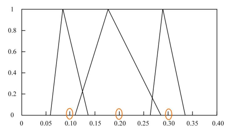
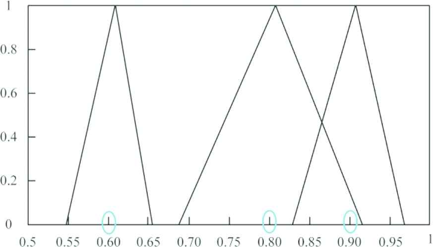
Figures 1 and 2 show that the normal fluctuation range of each possible value in HFE makes up a triangular region.
Example 1 illustrates the normal wiggly range is based on the assumption that DMs’ cognitive feelings fluctuate within the area of corresponding triangle. When the evaluation values provided by DMs less than 0.5, it means that they maintain pessimistic attitude toward the objects evaluated. On the contrary, optimistic DMs tend to give larger values to the objects. Over all, the NWHFSs can portray the deeper uncertain information hidden in DMs’ original evaluation values. Therefore, the NWHFS takes both original hesitant fuzzy information and potential concealed information into consideration.
Definition 3.
[7] Let
Definition 4.
[7] Let
Remark 1.
The score function of NWHFE in Ren et al. [7] neglected brackets and we correct it in Eq. (6).
Remark 2.
For any two NWHFEs
Definition 5.
[7] Let
In addition, the normal wiggly hesitant fuzzy weighted geometric (NWHFWG) operator can be defined as
3. IMPROVED BWM-BASED WEIGHT-DETERMINING APPROACH WITH NWHF INFORMATION
Usually, there may exist disagreements among the DMs, hence they shall make different assessments over the same objects based on their professional background. It is hard to represent their attitude by crisp evaluation values, consequently, HFS would be a good theory to reflect DMs’ hesitant decision information. However, if considering the concealed information of DMs, NWHFS could be used to dig the subjective preferences of them as well as contain the original information. In this paper, the BWM-based weight-determining approach can be divided into two parts. We can derive the weight vector of expert panel by BWM with NWHF information, and based on which, the optimal weights of criteria will be determined. Suppose there is an expert panel
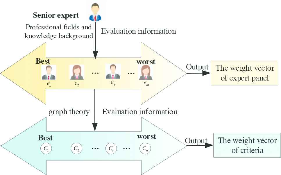
Improved best-worst method (BWM)-based weight-determining process with normal wiggly hesitant fuzzy (NWHF) information.
3.1. Construct the BWM-Based Weighting Model of Expert Panel
Motivated by [27] and [28], the weight vector of expert panel is determined by senior expert. In this paper, we describe the evaluation process in terms of NWHF information, which is different from the decision-making structure proposed by Hafezalkotob et al. [28]. We illustrate the steps as follows:
Step 1. For different decision-making problems, the senior expert selects the best and worst experts in the panel by analyzing their professional fields and knowledge background.
Step 2. In the improved BWM, the normal wiggly hesitant fuzzy best-to-others (NWHFBO) vector evaluated by senior expert can be represented in NWHFEs, which include a set of possible preference degrees in elements:
Step 3. The normal wiggly hesitant fuzzy others-to-worst (NWHFOW) vector can be represented as
Step 4. Inspired by [30], assuming that the multiple values in NWHFEs are evenly distributed, the score function could represent the most possible value, and can be used to reduce the computational complexity. Construct novel preference degrees by using Eq. (6) to convert the NWHFBO and NWHFOW vectors into the score-based NWHFBO and NWHFOW vectors, respectively. Therefore, the score-based NWHFBO and NWHFOW vectors can be denoted as follows:
Step 5. Suppose that the optimal weight vector of expert panel is
Then, we introduce the slack variable
Thus, if the slack variable
3.2. Construct the BWM-Based Weighting Model of Criteria
The weight vector of criteria is profoundly influenced by the expertise degrees of DMs. Therefore, along with the BWM-based weighting model of expert panel, we construct the weighting model of criteria as follows:
Step 1. Each expert in the panel picks out the best and worst criteria. In this regard, they could select the reference criteria based on the graph theory [49] with their professional knowledge and background.
Step 2. Experts give their NWHF preference degrees of the best criterion over each criterion i. The NWHFBO vector of criteria evaluated by the expert j can be represented as
Step 3. Experts give their NWHF preference degrees of the worst criterion over each criterion i. The NWHFOW vector of criteria evaluated by the expert j can be represented as
Step 4. Convert the NWHFBO and NWHFOW vectors of criteria into the score-based forms by using Eq. (6). Then the score-based NWHFBO and NWHFOW vectors of criteria evaluated by the expert j can be described as follows:
Step 5. Based on the multiplicative consistent relation, construct the BWM-based weighting model of criteria to calculate the optimal weight vector as follows:
Here, we can get the linear model (21) with the unique optimal weight vector
4. NOVEL DISTANCE MEASURES BETWEEN NWHFSs AND GROUP MULTIMOORA METHOD
In order to enhance the robustness of the evaluation results, we integrate a novel group MULTIMOORA method with NWHF information. However, to our best knowledge, no one has ever investigated the distance measures of NWHFSs, especially for integrating it with MULTIMOORA method. In this section, we put forward a various of novel distance measures between NWHFSs to develop the group MULTIMOORA method. In addition, we present a NWHF-ranking position method to aggregate the subordinate model ranking results of MULTIMOORA.
4.1. Novel Distances Measures between NWHFSs
Definition 6.
For a NWHFS in reference set X, the mean normal wiggly element (MNWE) can be denoted as
Definition 7.
Motivated by [48], let A and B be two NWHFSs on a reference set
It notes that the number of values in different NWHFEs may be different. For two NWHFSs A and B, in most cases,
Let C be any NWHFS, the NWHFEs of A, B and C have the same length
Definition 8.
For a reference set
The weighted Euclidean distance measure between A and B can be defined as
And the weighted generalized distance measure between A and B can be defined as
Remark 3.
NWE has the similar structure to hesitant triangular fuzzy element (HTFE). However, according to [51], when calculating the distance measures between HTFSs, it should be first converted to the corresponding HFSs. On the contrary, NWEs are mined from the original HFEs, therefore, it is not necessary to convert the NWEs into the corresponding HFEs.
4.2. The Group MULTIMOORA with NWHF-Ranking Position Method
Brauers and Zavadskas [31] first came up with the MULTIMOORA method to deal with the decision-making problem. Although MULTIMOORA is a good tool to investigate the real-life MCGDM problems, there is no research integrates the MULTIMOORA with NWHF information. In this paper, a group NWHF-MULTIMOORA theory is proposed. Besides, we put forward a NWHF-ranking position method to fuse the subordinate rankings. The group MULTIMOORA method involves following steps.
Step 1. Assuming that
Step 2. According to the NWHFWA operator, we can aggregate the NWHFEs provided by different experts into the following one:
Thus, the final group NWHF decision matrix can be denoted as

The aggregation process with normal wiggly hesitant fuzzy (NWHF) information.
Step 3. (Ratio system) The NWHFEs
The overall utility of the kth alternative based on the ratio system can be obtained as follows:
All of alternatives ranked by the descending order of
Step 4. (Reference point approach) We use the pessimistic principle to extend the shorter NWHFEs in the final NWHF decision matrix. Then, determining the reference point values according to the different types of criteria. The reference point values under the benefit type of criteria can be obtained as
And the reference point values under the cost type of criteria can be obtained as
Considering the weight vector of criteria, the NWHF weighted hamming distance
Then the NWHF evaluation values based on the reference point approach can be obtained as follows:
All the alternatives ranked by the ascending order of
Step 5. (Full multiplicative form) The NWHFEs
Then the NWHF evaluation values based on the full multiplicative form can be calculated as follows:
All of alternatives ranked by the descending order of
Step 6. Appropriate aggregation method could effectively ingrate the three subordinate ranking results, Luo and Li [37] recently proposed the improved ranking position method, which can combine the evaluation values and rankings into final evaluation values. In this paper, we present the NWHF-ranking position method to aggregate the subordinate utility values (
To use the NWHF-ranking position method, the evaluation values should be first normalized, that is,
By utilizing Eq. (38), all the alternatives ranked by the ascending order of
5. THE MCGDM ALGORITHM BASED ON BWM AND MULTIMOORA WITH NWHF INFORMATION
The framework of the proposed algorithm is shown in Figure 5, and details are illustrated in this section.
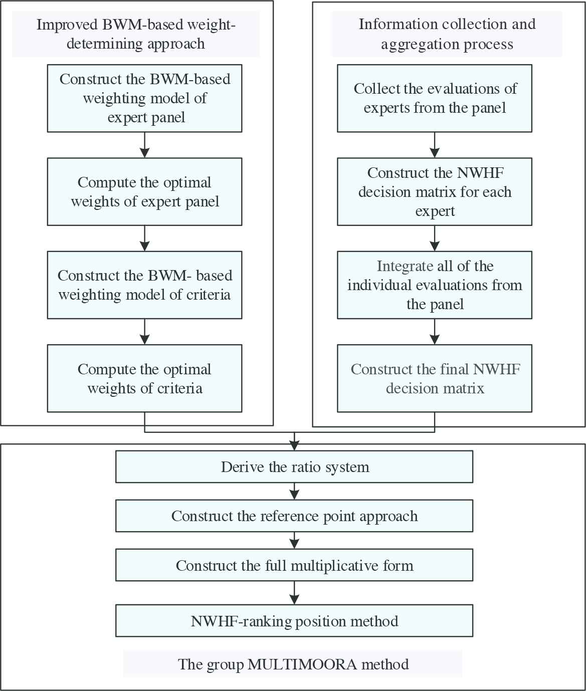
The framework of multi-criteria group decision-making algorithm.
Step 1. Select and identify the types of criteria, then determine the expert panel and senior expert.
Step 2. Construct the BWM-based weighting model of expert panel with NWHF information provided by senior expert. The optimal weights of expert can be obtained by the model (15).
Step 3. Based on the weights of experts, constructing the BWM-based weighting model of criteria with NWHF information provided by expert panel. Then the optimal weights of criteria can be computed by the model (21).
Step 4. Experts provide their evaluations for each alternative under criteria by NWHFEs and integrate them into the individual NWHF decision matrices by Eq. (25). Then, fuse all of the individual NWHF decision matrices into final group NWHF decision matrix by using NWHFWA operator.
Step 5. Determine the subordinate rankings of MULTIMOORA method by Eqs. (28), (32) and (36), and aggregate them by NWHF-ranking position method (38). Finally obtain the ranking result of alternatives and select the best one.
The MCGDM algorithm comprehensively reflects experts’ evaluation information, which includes original information and deeper potential preferences contained in the original hesitant fuzzy information. In addition, the improved BWM based on NWHF information could decrease the times of pairwise comparisons compared with AHP, that is to say, the redundant comparisons of AHP are eliminated. Moreover, MULTIMOORA includes three approaches, which means it is more robust than other multi-objective optimization systems. Apart from that, the NWHF-ranking position method provides a more reasonable way to integrate the subordinate rankings by taking account into both evaluation values and ranking results.
6. CASE STUDY: TRAIN SELECTION DURING THE SPRING FESTIVAL TRAVEL RUSH
The Spring Festival is one of the most important traditional festivals in China. Since many Chinese people study or work in the big cities, they return to their hometowns to reunite with their families during the period. The largest annual human migration that hundreds of millions of people joined in leads to a unique phenomenon, which is named as the Spring Festival travel rush. The official press released that approximately 2.98 billion people migrated during the 40-day Spring Festival travel rush in 2019. Meanwhile, for the intensive railway network and improving high-speed rail in China, most people tend to choose trains as their returning tool. However, the railway system of China also faces huge challenges during the peak period, which include the difficulty of buying tickets, high probability of delay and the heavy traffic congestion. Therefore, it is necessary for returning passengers to choose reasonable trains, and try to save time while taking the comfort of travel into account.
6.1. Improved BWM-MULTIMOORA Approach with NWHF Information for Train Selection Research
Taking the Spring Festival travel rush in 2019 as an example for analysis. By querying the official website database of China National Railway Group Co., Ltd. (see www.12306.cn), we select one of the most popular routes during the Spring Festival travel period, i.e., “Shanghai-Weinan Railway” as the research object. Weinan City is an important labor export area in Shaanxi Province, China. In 2019, the number of migrant workers in Weinan City reached 956000. Given the composition of this route, we consider a candidate alternative set containing two high-speed and two local trains. In this paper, the high-speed train is that whose number starts with H or D, while the number of local trains start with Z or K. Table 1 shows the background information of the four trains on January 30, 2019.
| Travel Scenario Number | Train Number | Ticket Price | Ticket Type | Travel Time | Arrival Time | Delay Time(min) | Ticket Sold-Out Time (s) |
|---|---|---|---|---|---|---|---|
| K2186 | ¥304.5 | Berth ticket | 20 h 59 min (cross the night) | 8:00 AM | 10 | 43 | |
| G1970 | ¥643.5 | Second class | 6 h 52 min | 1:00 PM | 0 | 32 | |
| Z92 | ¥177.5 | Hard-seat | 14 h 34 min (cross the night) | 8:30 PM | 4 | 50 | |
| D306 | ¥439.5 | Second class | 10 h 49 min (cross the night) | 9:30 PM | 0 | 37 |
Background information of the four trains on January 30, 2019.
Train selection during the Spring Festival travel rush is a MCGDM problem with respect of the quality and speed of travel. Therefore, this study can be conducted on the basis of the algorithm proposed in Section 5.
Step 1. In the process of choosing the most suitable train during the Spring Festival travel rush by passengers, many factors should be taken into account in order to make a reasonable decision. A comprehensive criteria system can help DMs get the scientific decision results. Thus, we construct a criteria set to evaluate the multiple alternative trains, which including total travel time
Total travel time
Total travel time is a significant criterion that should be extensively took into account. For instance, the high-speed train usually has higher speed and on-time performance than local train does, which can save passengers’ time during the process of returning hometowns. However, for the passengers with flexible schedules, since delay is already expected, they may have greater tolerance for delay. In general, along with the total travel time reducing, the satisfaction of those passengers who experience the crowded travel is increased gradually. Therefore,
Travel expenses
The travel expenses could profoundly affect passengers’ selection. Although taking local train lead to longer travel time, the lower ticket fare could attract some budget-conscious passengers. In addition, the cross-night local train service with berth ticket is more economical, because it provides the hard sleeper facilities which save the hotel rate for passengers one night. Overall, passengers are more likely to choose a cheaper way of travel under the same conditions, and thus,
Comfort
Passengers’ comfort is an important criterion for measuring trains. Comparing with the cross-night local train and high-speed train without sleeper facilities, the berth ticket of local train is more comfortable. Besides, for a day trip, there is no doubt that the hardware facilities of high-speed trains are more complete than those of local trains, which will bring a better travel experience. Therefore, we summarize this factor as the benefit criterion.
The difficulty of purchasing tickets
During the Spring Festival period when tickets are in short supply, the difficulty of purchasing tickets determines whether passengers can arrive their hometown on time. The shorter sold-out time means that one ticket for this train is difficult to be found. Hence,
| Criteria | Reference Information | Types |
|---|---|---|
| Travel time, arrival time and delay time | Cost | |
| Ticket price of trains | Cost | |
| Ticket types of trains | Benefit | |
| Ticket sold-out time | Benefit |
Reference information and types of criteria.
A panel with four experts, which include an operations researcher (
Step 2. The senior expert determines the weights of expert panel by NWHF preference degrees. The corresponding NWHF preference degrees considered by the senior expert are shown in Table 3. Indeed, Table 3 lists the NWHFBO and NWHFOW vectors of the experts’ weights. Then, construct the novel NWHF preferences by converting NWHFBO vectors and NWHFOW vectors into score-based forms by using Eq. (6). Table 4 shows the corresponding score-based NWHF preferences determined by the senior expert. The optimal weights of expert panel can be computed by solving model (15), and the results with respect to different level of confidence are shown in Table 5.
| Best: |
<(0.7, 0.8), {(0.67, 0.70, 0.73), (0.77, 0.80, 0.83)}> | <(0.6, 0.7, 0.8), {(0.33, 0.41, 0.47), (0.54, 0.73, 0.86), (0.70, 0.82, 0.91)}> | <(0.5), {(0.5, 0.5, 0.5)}> | <(0.8, 0.9), {(0.77, 0.80, 0.83), (0.87, 0.9, 0.93)}> |
| Worst: |
<(0.5, 0.7, 0.8), {(0.45, 0.51, 0.55), (0.58, 0.72, 0.82), (0.73, 0.81, 0.87}> | <(0.5, 0.8, 0.9), {(0.43, 0.51, 0.57), (0.64, 0.83, 0.96), (0.79, 0.92, 1)}> | <(0.8, 0.9), {(0.77, 0.80, 0.83), (0.87, 0.9, 0.93)}> | <(0.5), {(0.5, 0.5, 0.5)}> |
Senior expert’s normal wiggly hesitant fuzzy (NWHF)normal wiggly hesitant fuzzy preference degrees of the expert panel.
| Best and Worst Experts | |||||||||
|---|---|---|---|---|---|---|---|---|---|
| Best: Worst: |
0.1 | 0.734 | 0.684 | 0.5 | 0.843 | 0.638 | 0.686 | 0.843 | 0.5 |
| 0.3 | 0.733 | 0.670 | 0.5 | 0.834 | 0.617 | 0.659 | 0.834 | 0.5 | |
| 0.5 | 0.724 | 0.655 | 0.5 | 0.824 | 0.595 | 0.631 | 0.824 | 0.5 | |
| 0.7 | 0.714 | 0.640 | 0.5 | 0.814 | 0.574 | 0.604 | 0.814 | 0.5 | |
| 0.9 | 0.705 | 0.626 | 0.5 | 0.805 | 0.553 | 0.577 | 0.805 | 0.5 | |
NWHF, normal wiggly hesitant fuzzy; NWHFBO, normal wiggly hesitant fuzzy best-to-others; NWHFOW, normal wiggly hesitant fuzzy others-to-worst.
Senior expert’s score-based NWHF preference degrees of the expert panel.
| Optimal Weights of Experts |
|||||
|---|---|---|---|---|---|
| 0.1 | 0.0040 | 0.182 | 0.224 | 0.497 | 0.097 |
| 0.3 | 0.0079 | 0.18 | 0.228 | 0.486 | 0.106 |
| 0.5 | 0.0121 | 0.193 | 0.227 | 0.466 | 0.114 |
| 0.7 | 0.0164 | 0.202 | 0.227 | 0.449 | 0.122 |
| 0.9 | 0.0206 | 0.207 | 0.227 | 0.435 | 0.131 |
The optimal weights of expert panel.
In the following, we assume that the confidence level of all experts in original evaluation information is 0.5, i.e.,
Step 3. According to the improved BWM-based weighting model of criteria, four experts rate their NWHF preference degrees of criteria regarding to the best and worst criteria, respectively. The corresponding NWHF preferences considered by the expert panel are shown in Appendix A (Tables A1–A4). Tables A1–A4 list the NWHFBO and NWHFOW vectors of preference degrees of criteria. Then, we convert NWHFBO and NWHFOW vectors of criteria into score-base forms, as shown in Table 6.
| Experts | Criteria Types |
|||||||||
|---|---|---|---|---|---|---|---|---|---|---|
| Best | Worst | |||||||||
| 0.5 | 0.624 | 0.9 | 0.834 | 0.9 | 0.746 | 0.5 | 0.524 | |||
| 0.555 | 0.5 | 0.655 | 0.824 | 0.755 | 0.824 | 0.524 | 0.5 | |||
| 0.5 | 0.566 | 0.746 | 0.9 | 0.9 | 0.724 | 0.655 | 0.5 | |||
| 0.5 | 0.655 | 1 | 0.695 | 1 | 0.631 | 0.5 | 0.566 | |||
NWHF, normal wiggly hesitant fuzzy; NWHFBO, normal wiggly hesitant fuzzy best-to-others; NWHFOW, normal wiggly hesitant fuzzy others-to-worst.
Experts’ score-based NWHF preference degrees of the criteria (
Solving model (21), the optimal weights of criteria are 0.45, 0.354, 0.108 and 0.088, and the objective value
Step 4. Experts (
| <(0.66,…), {(0.61, 0.67, 0.71),…}> | <(0.25,…), {(0.19, 0.24, 0.31),…}> | <(0.48,…), {(0.45, 0.48, 0.51),…}> | <(0.38,…), {(0.32, 0.39, 0.44),…}> | |
| <(0.61,…), {(0.56, 0.62, 0.66),…}> | <(0.79,…), {(0.76, 0.79, 0.82),…}> | <(0.6,…), {(0.55, 0.6, 0.65),…}> | <(0.56,…), {(0.5, 0.57, 0.62),…}> | |
| <(0.24,…), {(0.16, 0.24, 0.32),…}> | <(0.44,…), {(0.4, 0.44, 0.48),…}> | <(0.63,…), {(0.55, 0.64, 0.71),…}> | <(0.27,…), {(0.16, 0.24, 0.38),…}> | |
| <(0.54,…), {(0.47, 0.55, 0.61),…}> | <(0.24,…), {(0.16, 0.22, 0.32),…}> | <(0.66,…), {(0.61, 0.66, 0.71),…}> | <(0.62,…), {(0.58, 0.62, 0.66),…}> |
NWHF, normal wiggly hesitant fuzzy; HFE, hesitant fuzzy element; NEW, normal wiggly element.
The final group NWHF decision matrix (only the first value in HFE and in NWE is shown).
Step 5. Table 8 lists the evaluation values and ranking results for the MULTIMOORA method, consisted of ratio system, reference point model and full multiplicative form, based on Eqs. (28), (32) and (36). By using Eq. (38),
| Trains | NWHFRT |
NWHFRP |
NWHFFMF |
|||
|---|---|---|---|---|---|---|
| 0.276 | 3 | 0.143 | 1 | 0.447 | 1 | |
| 0.471 | 1 | 0.397 | 4 | 0.283 | 2 | |
| 0.384 | 2 | 0.262 | 2 | 0.182 | 4 | |
| 0.070 | 4 | 0.392 | 3 | 0.233 | 3 | |
NWHFRT, normal wiggly hesitant fuzzy ratio system; NWHFRP, normal wiggly hesitant fuzzy reference point; NWHFFMF, normal wiggly hesitant fuzzy full multiplicative form.
Evaluation values and rankings of the subordinate models of group MULTIMOORA.
According to the weighting model of criteria, we can get the conclusion that DMs pay more attention to the impact of travel time on train selection. Therefore, most passengers are inclined to choose high-speed train as their return tool in order to rush home as soon as possible. It provides the guidance that the Chinese government should add more extra high-speed trains and increase their frequency of departures during the Spring Festival.
6.2. Comparison Analysis
To verify the advantages and feasibility of the proposed approach in this paper, we compare the proposed method with the normal wiggly hesitant fuzzy weighted averaging (NWHFWA) operator and the normal wiggly hesitant fuzzy weighted geometric (NWHFGA) operator. Ren et al. [7] takes advantage of different aggregation operators to integrate decision matrices, and then uses score function to characterize the pros and cons of the alternatives. In the decision-making method of [7], the decision matrices and the weights of criteria and experts are computed by the proposed method in this paper.
The rankings obtained by the three approaches are shown in Table 9. Evidently, ranking results computed by Ren et al. [7]’s method are roughly the same as the approach in this paper, which validates the efficiency of the proposed method. However, we find that the ranking of
| Trains | NWHFWA | Ranking | NWHFGA | Ranking | The Proposed Approach |
|---|---|---|---|---|---|
| 0.379 | 2 | 0.344 | 3 | 2 | |
| 0.392 | 1 | 0.427 | 1 | 1 | |
| 0.233 | 3 | 0.358 | 2 | 3 | |
| 0.212 | 4 | 0.274 | 4 | 4 |
NWHFWA, normal wiggly hesitant fuzzy weighted averaging; NWHFGA, normal wiggly hesitant fuzzy weighted geometric.
Ranking results of different approaches.
7. CONCLUSIONS
MCGDM problems are widespread in daily life. However, it is difficul for the DMs in reaching a certain consensus of a crisp value in membership degree. For purpose of avoiding loss evaluation data and digging the potential information related to original evaluations, we introduce the NWHFS theory, which can describe the feelings of DMs more comprehensively. In this paper, an integrated improved BWM and MULTIMOORA method under the NWHF environment has been proposed to solve MCGDM issues. For completing the approach, we construct an improved BWM based on the score function of NWHFS. Due to the weights of criteria is influenced by the expertise degrees of DMs, we derive a novel BWM-based weighting model of criteria on the basis of experts’ weight vector. Then we present some distance measures between NWHFSs and discuss their properties. According to these distance measures and NWHFWA operators, a group MULTIMOORA method with NWHF information is put forward. Then, a novel aggregation methodology, named NWHF-ranking position method, is employed the subordinate ranking results of MULTIMOORA method. Besides, we summarize the proposed method’s specific application steps, and apply it to the issue of train selection during the Spring Festival travel rush. The ranking results indicate that the government should increase the operation and construction of high-speed rail in order to provide enough trains during the Spring Festival. Finally, through the comparison analysis with Ren et al. [7]’s method, we demonstrate the validity and effectiveness of our approach.
The superiorities of this work can be manifested as follows: (1) Solving MCGDM problems by using NWHF information not only remains the original evaluation possible values in membership degree, but also digs the potential uncertain information. (2) The improved BWM based on the score function of NWHFS can obtain the weight vectors more conveniently. (3) The novel MULTIMOORA along with its NWHF-ranking position method make the final results more convincing by fusing the subordinate rankings and evaluation values. (4) We establish a comprehensive criteria system to evaluate the problem of train selection during the Spring Festival travel rush. And the proposed method is applied to a specific case, which can guide the Chinese government to formulate a reasonable response strategy.
In the future, we will focus on studying the extension of NWHFS so that the expression of DMs could be more accurate. Apart from that, we will investigate the deep psychological factors of passengers during the Spring Festival travel rush, so as to establish a set of more objective evaluation criteria.
CONFLICT OF INTEREST
The authors declare no conflicts of interest.
AUTHOR'S CONTRIBUTIONS
Chengxiu Yang: Conceptualization, methodology, investigation, data curation, writing—original draft preparation, writing—review and editing.
Qianzhe Wang: Conceptualization, writing—review and editing.
Weidong Peng: Methodology, investigation, supervision.
Jie Zhu: Software, investigation, funding acquisition.
ACKONWLEDGMENTS
This work was supported in part by the National Natural Science Foundation of China (NSFC) under Grant 61773197, and in part by the Shaanxi Province Lab. of Meta synthesis for Electronic and Information System.
APPENDIX A
Appendix A shows the normal wiggly hesitant fuzzy best-to-others (NWHFBO) and wiggly hesitant fuzzy others-to-worst (NWHFOW) vectors of preference degrees of criteria.
| Best criterion |
<(0.5), {(0.5, 0.5, 0.5)}> | <(0.6, 0.7), {(0.57, 0.60, 0.63), (0.67, 0.70, 0.73)}> | <(0.9), {(0.9, 0.9, 0.9)}> | <(0.8, 0.9), {(0.77, 0.80, 0.83), (0.87, 0.90, 0.93)}> |
| Worst criterion |
<(0.9), {(0.9, 0.9, 0.9)}> | <(0.7, 0.9), {(0.64, 0.71, 0.76), (0.84, 0.91, 0.96)}> | <(0.5), {(0.5, 0.5, 0.5)}> | <(0.5, 0.6), {(0.47, 0.50, 0.53), (0.57, 0.60, 0.63)}> |
Expert
| Best criterion |
<(0.5, 0.7, 0.8), {(0.45, 0.51, 0.55), (0.58, 0.71, 0.82), (0.73, 0.81, 0.87}> | <(0.5), {(0.5, 0.5, 0.5)}> | <(0.6, 0.7, 0.8), {(0.56, 0.60, 0.64), (0.62, 0.71, 0.78), (0.76, 0.80, 0.84)}> | <(0.8, 0.9), {(0.77, 0.80, 0.83), (0.87, 0.90, 0.93)}> |
| Worst criterion |
<(0.7, 0.8, 0.9), {(0.66, 0.70, 0.74), (0.72, 0.81, 0.88), (0.86, 0.90, 0.94)}> | <(0.8, 0.9), {(0.77, 0.80, 0.83), (0.87, 0.90, 0.93)}> | <(0.5, 0.6), {(0.47, 0.50, 0.53), (0.57, 0.60, 0.63)}> | <(0.5), {(0.5, 0.5, 0.5)}> |
Expert
| Best criterion |
<(0.5), {(0.5, 0.5, 0.5)}> | <(0.5, 0.8), {(0.41, 0.52, 0.59), (0.71, 0.82, 0.89)}> | <(0.7, 0.9), {(0.64, 0.71, 0.76), (0.84, 0.91, 0.96)}> | <(0.9), {(0.9, 0.9, 0.9)}> |
| Worst criterion |
<(0.9), {(0.9, 0.9, 0.9)}> | <(0.7, 0.8), {(0.67, 0.70, 0.73), (0.77, 0.80, 0.83)}> | <(0.6, 0.7, 0.8), {(0.56, 0.60, 0.64), (0.62, 0.71, 0.78), (0.76, 0.80, 0.84)}> | <(0.5), {(0.5, 0.5, 0.5)}> |
Expert
| Best criterion |
<(0.5), {(0.5, 0.5, 0.5)}> | <(0.6, 0.7, 0.8), {(0.56, 0.60, 0.64), (0.62, 0.71, 0.78), (0.76, 0.80, 0.84)}> | <(1), {(1, 1, 1)}> | <(0.6, 0.8, 0.9), {(0.55, 0.61, 0.57), (0.64, 0.83, 0.96), (0.80, 0.92, 1)}> |
| Worst criterion |
<(1), {(1, 1, 1)}> | <(0.5, 0.8, 0.9), {(0.43, 0.51, 0.66), (0.68, 0.82, 0.92), (0.83, 0.91, 0.97)}> | <(0.5), {(0.5, 0.5, 0.5)}> | <(0.5, 0.8), {(0.41, 0.52, 0.59), (0.71, 0.82, 0.89)}> |
Expert
APPENDIX B
Appendix B shows expert panel’s normal wiggly hesitant fuzzy (NWHF) decision matrices.
| <(0.7, 0.9), {(0.64, 0.71, 0.76), (0.84, 0.91, 0.96)}> | <(0.6), {(0.6, 0.6, 0.6)}> | <(0.5, 0.8), {(0.41, 0.52, 0.59), (0.71, 0.82, 0.89)}> | <(0.4, 0.7, 0.8), {(0.33, 0.41, 0.47), (0.54, 0.73, 0.86), (0.69, 0.82, 0.90)}> | |
| <(0.5, 0.6), {(0.47, 0.50, 0.53), (0.57, 0.60, 0.63)}> | <(0.8), {(0.8, 0.8, 0.8)}> | <(0.4, 0.6), {(0.34, 0.4, 0.46), (0.54, 0.6, 0.66}> | <(0.5, 0.7, 0.8), {(0.45, 0.51, 0.55), (0.58, 0.72, 0.82), (0.73, 0.81, 0.87}> | |
| <(0.3), {(0.3, 0.3, 0.3)}> | <(0.5), {(0.5, 0.5, 0.5)}> | <(0.6, 0.7, 0.8), {(0.56, 0.60, 0.64), (0.62, 0.71, 0.78), (0.76, 0.80, 0.84)}> | <(0.2, 0.3, 0.4), {(0.16, 0.19, 0.24), (0.2, 0.28, 0.38), (0.36, 0.39, 0.44)}> | |
| <(0.5, 0.8, 0.9), {(0.43, 0.51, 0.57), (0.64, 0.83, 0.96), (0.79, 0.91, 1)}> | <(0.2, 0.4), {(0.14, 0.18, 0.2), (0.34, 0.38, 0.46)}> | <(0.8, 0.9), {(0.77, 0.80, 0.83), (0.87, 0.90, 0.93)}> | <(0.3, 0.5), {(0.24, 0.29, 0.36), (0.44, 0.48, 0.56)}> |
Expert
| <(0.4, 0.7, 0.9), {(0.31, 0.42, 0.49), (0.50, 0.75, 0.90), (0.79, 0.93, 1)}> | <(0.3, 0.6), {(0.21, 0.27, 0.40), (0.51, 0.57, 0.69)}> | <(0.4, 0.5, 0.8), {(0.29, 0.42, 0.51), (0.34, 0.54, 0.66), (0.73, 0.82, 0.87)}> | <(0.2, 0.4), {(0.14, 0.18, 0.26), (0.34, 0.38, 0.46)}> | |
| <(0.4, 0.6), { (0.34, 0.4, 0.46), (0.54, 0.6, 0.66}> | <(0.8, 0.9), {(0.77, 0.80, 0.83), (0.87, 0.90, 0.93)}> | <(0.3, 0.4), {(0.27, 0.30, 0.33), (0.37, 0.40, 0.43))}> | <(0.7), {(0.7, 0.7, 0.7)}> | |
| <(0.4, 0.6), { (0.34, 0.4, 0.46), (0.54, 0.6, 0.66}> | <(0.3, 0.6), {(0.21, 0.27, 0.39), (0.51, 0.57, 0.69)}> | <(0.7), {(0.7, 0.7, 0.7)}> | <(0.3, 0.6), {(0.21, 0.27, 0.39), (0.51, 0.57, 0.69)}> | |
| <(0.4, 0.7, 0.8), {(0.33, 0.41, 0.47), (0.54, 0.73, 0.86), (0.69, 0.82, 0.91)}> | <(0.5, 0.6), {(0.47, 0.50, 0.53), (0.57, 0.60, 0.63)}> | <(0.9), {(0.9, 0.9, 0.9)}> | <(0.4, 0.7), {(0.31, 0.42, 0.49), (0.61, 0.72, 0.79)}> |
Expert
| <(0.8, 0.9), {(0.77, 0.80, 0.83), (0.87, 0.90, 0.93)}> | <(0.2, 0.3), {(0.17, 0.19, 0.23), (0.27, 0.29, 0.33)}> | <(0.3, 0.6), {(0.21, 0.27, 0.39), (0.51, 0.57, 0.69)}> | <(0.4), {(0.4, 0.4, 0.4)}> | |
| <(0.6, 0.9), {(0.51, 0.62, 0.69), (0.81, 0.82, 0.99)}> | <(0.7, 0.9), {(0.64, 0.71, 0.76), (0.84, 0.91, 0.96)}> | <(0.6), {(0.6, 0.6, 0.6)}> | <(0.8), {(0.8, 0.8, 0.8)}> | |
| <(0.2, 0.4), {(0.14, 0.18, 0.26), (0.34, 0.38, 0.46)}> | <(0.5, 0.6), {(0.47, 0.50, 0.53), (0.57, 0.60, 0.63)}> | <(0.6, 0.7, 0.8), {(0.56, 0.60, 0.64), (0.62, 0.71, 0.78), (0.76, 0.80, 0.84)}> | <(0.2, 0.6), {(0.08, 0.14, 0.32), (0.48, 0.54, 0.72)}> | |
| <(0.7, 0.9), {(0.64, 0.71, 0.76), (0.84, 0.97, 0.96)}> | <(0.2), {(0.2, 0.2, 0.2)}> | <(0.8), {(0.8, 0.8, 0.8)}> | <(0.1, 0.3), {(0.04, 0.07, 0.16), (0.24, 0.27, 0.36)}> |
Expert
| <(0.4, 0.7, 0.9), {(0.31, 0.42, 0.49), (0.50, 0.75, 0.90), (0.79, 0.93, 1)}> | <(0.3, 0.4), {(0.27, 0.30, 0.33), (0.37, 0.40, 0.43))}> | <(0.4, 0.6), { (0.34, 0.4, 0.46), (0.54, 0.6, 0.66}> | <(0.5), {(0.5, 0.5, 0.5)}> | |
| <(0.6, 0.9), {(0.51, 0.62, 0.69), (0.81, 0.82, 0.99)}> | <(0.7, 0.9), {(0.64, 0.71, 0.76), (0.84, 0.91, 0.96)}> | <(0.7), {(0.7, 0.7, 0.7)}> | <(0.8, 0.9), {(0.77, 0.80, 0.83), (0.87, 0.90, 0.93)}> | |
| <(0.1, 0.3), {(0.04, 0.07, 0.16), (0.24, 0.27, 0.36)}> | <(0.4, 0.6), {(0.4, 0.4, 0.46), (0.54, 0.6, 0.66}> | <(0.6), {(0.6, 0.6, 0.6)}> | <(0.3, 0.5, 0.6), {(0.25, 0.29, 0.35), (0.38, 0.47, 0.62), (0.53, 0.58, 0.67)}> | |
| <(0.2), {(0.2, 0.2, 0.2)}> | <(0.1, 0.4), {(0.01, 0.05, 0.19), (0.31, 0.35, 0.49)}> | <(0.5, 0.8), {(0.41, 0.52, 0.59), (0.71, 0.82, 0.89)}> | <(0.3, 0.5), {(0.24, 0.28, 0.36), (0.44, 0.48, 0.56)}> |
Expert
REFERENCES
Cite this article
TY  - JOUR
AU  - Chengxiu Yang
AU  - Qianzhe Wang
AU  - Weidong Peng
AU  - Jie Zhu
PY  - 2020
DA  - 2020/04/06
TI  - A Multi-Criteria Group Decision-Making Approach Based on Improved BWM and MULTIMOORA with Normal Wiggly Hesitant Fuzzy Information
JO  - International Journal of Computational Intelligence Systems
SP  - 366
EP  - 381
VL  - 13
IS  - 1
SN  - 1875-6883
UR  - https://doi.org/10.2991/ijcis.d.200325.001
DO  - 10.2991/ijcis.d.200325.001
ID  - Yang2020
ER  -