
A Novel Pythagorean Fuzzy LINMAP-Based Compromising Approach for Multiple Criteria Group Decision-Making with Preference Over Alternatives
- DOI
- 10.2991/ijcis.d.200408.001How to use a DOI?
- Keywords
- Compromising approach; Group decision-making; Pythagorean fuzzy set; LINMAP; Dominance measure
- Abstract
This paper presents a new compromising approach to multiple criteria group decision-making (MCGDM) for the treatment of uncertainty which is based on Pythagorean fuzzy (PF) sets. The present work intends to propose a novel linear programming technique for multidimensional analysis of preference (LINMAP) by way of some useful concepts related to PF dominance relations, individual consistency and inconsistency levels, and individual fit measurements. The concept of PF scalar function-based dominance measures is defined to conduct intracriterion comparisons concerning uncertain evaluation information based on Pythagorean fuzziness; moreover, several valuable properties are also investigated to demonstrate its effectiveness. For the assessment of overall dominance of alternatives, this paper provides a synthetic index, named a comprehensive dominance measure, which is the aggregation of the weighted dominance measures by combining unknown weight information and PF dominance measures of various criteria. For each decision-maker, this paper employs the proposed measures to evaluate the individual levels of rank consistency and rank inconsistency regarding the obtained overall dominance relations and the decision-maker's preference comparisons over paired alternatives. In the framework of individual fit measurements, this paper constructs bi-objective mathematical programming models and then provides their corresponding parametric linear programming models for generating the best compromise alternative. Realistic applications with some comparative analyses concerning railway project investment are implemented to demonstrate the appropriateness and usefulness of the proposed methodology in addressing actual MCGDM problems.
- Copyright
- © 2020 The Authors. Published by Atlantis Press SARL.
- Open Access
- This is an open access article distributed under the CC BY-NC 4.0 license (http://creativecommons.org/licenses/by-nc/4.0/).
1. INTRODUCTION
Multiple criteria group decision-making (MCGDM) intends to prioritize a set of candidate alternatives based on a set of evaluative criteria regarding subjective preference and judgments of multiple decision-makers. The linear programming technique for multidimensional analysis of preference (LINMAP) initiated by Srinivasan and Shocker [1] provides an efficient decision-making tool to address MCGDM problems with preference information over alternatives and unknown weights of criteria [2–4]. When decision-makers provide preference relations between pairs of alternatives in the MCGDM process, the LINMAP methods can be effectively applied to resolve the objective weights of criteria and specify the best compromise choice by ranking alternatives. According to preference relations through pairwise comparisons over alternatives, a linear programming model that desires to accomplish the minimum inconsistency is established in the LINMAP procedure to determine the optimal weights of criteria objectively and generate the priority ranking results of alternatives [5–7].
However, the classical LINMAP methods cannot be directly employed to handle the decision-making problems involving fuzzy information because of the uncertainty contained in performance information or evaluation values of candidate alternatives in terms of criteria [8–10]. Accordingly, numerous studies have extended the classical LINMAP for conducting multiple criteria decision analysis in a variety of different fuzzy circumstances. For example, Wan and Li [11] emanated from LINMAP to construct an intuitionistic fuzzy programming method for handling heterogeneous MCGDM containing intuitionistic fuzzy truth degrees. Furthermore, Wan and Li [8] considered the hesitancy degrees about pairwise comparisons as interval-valued intuitionistic fuzzy sets to establish a fuzzy LINMAP-based method for conducting a heterogeneous decision analysis. Zhang et al. [12] utilized the LINMAP and Shapley values to develop an interval-valued intuitionistic fuzzy mathematical programming model to manage uncertain MCGDM problems. Moreover, Zhang et al. [13] established a mathematical programming-based approach to heterogeneous MCGDM involving aspirations and incomplete preference information. Zhang and Xu [10] applied the LINMAP structure to present an interval programming method for handling MCGDM problems with hesitant fuzzy ratings of alternatives and pairwise judgments between alternatives using interval numbers. Wan et al. [14] developed a hesitant fuzzy mathematical programming model to deal with hybrid MCGDM involving hesitant fuzzy truth degrees and incomplete criteria weight information. Xu et al. [15] combined hesitant fuzzy linguistic term sets with LINMAP to provide a hesitant fuzzy linguistic LINMAP method. Liu et al. [5] explored a double-hierarchy hesitant fuzzy linguistic mathematical programming technique for MCGDM. To multiple criteria decision analysis, Gou et al. [6] proposed a hesitant fuzzy linguistic possibility degree-based linear assignment method and made some comparisons with a hesitant fuzzy LINMAP. Song et al. [7] solved a decision-making problem with multi-stage uncertain risk on the grounds of interval grey numbers and an extended LINMAP method. Liao et al. [16] established a linear programming model to address decision-making issues, where the decision-maker's preferences over alternatives in connection with criteria are described as probabilistic linguistic term sets. With the assistance of LINMAP, Qin et al. [17] constructed some linear programming models to solve an MCGDM problem in interval type-2 fuzzy contexts. Haghighi et al. [3] developed a soft computing model involving interval type-2 fuzzy information by the agency of a linear assignment method and LINMAP.
Vagueness and impreciseness are unavoidable uncertainties in human evaluation processes [18]. The concept of Pythagorean fuzzy (PF) sets, initiated by Yager [19–21] and Yager and Abbasov [22], is a powerful tool in handling real-world uncertainty because PF sets slacken the prerequisite in which the sum of membership and nonmembership degrees is less than or equal to one with the square sum is less than or equal to one [23–25]. Accordingly, PF sets allow decision-makers to portray uncertain assessment data agilely and conveniently during the MCGDM process.
The LINMAP methodology has been successfully extended to diverse uncertain representations for conducting multiple criteria decision analysis or handling MCGDM issues under a variety of distinct fuzzy environments. Nonetheless, most of the current LINMAP-based techniques are not applicable to the decision environments under complex uncertainty of Pythagorean fuzziness. In this regard, Wan et al. [9] and Xue et al. [26] put forward new LINMAP-based techniques in PF uncertain circumstances. Wan et al. [9] utilized the information entropy to derive individual subjective criterion weight vectors for multiple decision-makers and synthesized them into a collective one via a cross-entropy optimization model. Subsequently, Wan et al. [9] constructed a PF mathematical programming model for addressing MCGDM problems based on the PF truth degree. Xue et al. [26] defined new PF entropy measures and exploited a PF LINMAP method for solving MCGDM problems. These two studies have made significant contributions to enrich the theory of PF sets and have been applied to diverse fields of green supplier selection of a smelting equipment [9] and the selection of railway project investment [26]. In contrast to abovementioned information entropy-based techniques, this paper adopts the perspective of PF representation to construct the core concept in the PF LINMAP framework. Different from Wan et al. [9] and Xue et al. [26], this paper intends to employ the concept of PF scalar functions from fuzzy rule bases and develop a novel PF LINMAP-based compromising approach to deal with MCGDM problems within PF decision environments.
It is worthwhile to mention that the concept of PF scalar functions presented by Yager [19,20] and Yager and Abbasov [22] can be utilized to facilitate comparisons among complicated PF information. Yager [20] and Yager and Abbasov [22] explored the relationship between complex numbers and Pythagorean membership grades; then they demonstrated that Pythagorean membership grades are regarded as a subclass of complex numbers called Π−i numbers. Moreover, they introduced a mapping, i.e., a PF scalar function, from the Π−i numbers to the unit intervals to enhance the usage of PF sets in the decision-making field. Liu and Zhang [27] further demonstrated several useful properties of PF scalar functions and obtained some partial orders on Π−i numbers based on such functions. Zeng et al. [28] introduced the following four commonly used approaches to comparing and ranking Pythagorean membership grades in PF sets: the approach via score functions [29], the approach via score functions and accuracy functions [30], the approach via closeness indices [31], and the approach via PF scalar functions [20]. Zeng et al. [28] investigated several comparative examples and indicated that the approach by virtue of PF scalar functions is more helpful than the other existing comparison approaches. Consistent with Zeng et al.'s findings, Li and Zeng [32] also validated the effectiveness and superiority of PF scalar functions in comparing complex PF information. Moreover, Li and Zeng [32] and Zeng et al. [28] mentioned that the PF scalar function can thoroughly consider the influence of the fundamental characteristics of PF information. On the grounds of the PF scalar function in terms of certain anchor points of reference, Chen [33] introduced the measurement of PF precedence indices and precedence-based preference functions and further established a new PF preference ranking organization method for enrichment evaluations (PROMETHEE). Chen demonstrated the usefulness and effectiveness of the PF scalar function because its based PF precedence index can simplify the data-processing procedure and avoid the loss of high-order uncertain information. The previous studies indicated the merits of PF scalar functions; it would be desirable to apply the PF scalar function-based method to address intricate decision-making problems. Nevertheless, the concept of PF scalar functions has not employed in the current LINMAP-based methods within PF decision environments. Considering the benefits of the PF scalar function in measuring the magnitudes of Pythagorean membership grades as well as the usefulness of comparisons of PF information, this paper utilizes the PF scalar functions to present PF scalar function-based dominance measures that form the PF LINMAP basis for building a strong foundation of valuable concepts related to PF dominance relations, individual consistency and inconsistency levels, and individual fit measurements.
The primary purpose of this paper is to exploit an innovative PF LINMAP-based compromising approach for coping with MCGDM problems within PF environment. More fundamentally, this paper fully utilizes the essential characteristics of PF sets and provides a PF scalar function-based approach for determining PF dominance relations and building a core structure of the PF LINMAP procedure. First, the idea of PF scalar functions is fully employed to construct two types of PF scalar function-based dominance measures with respective to displaced and fixed reference points. Next, Types I and II comprehensive dominance measures are established for the sake of determining PF dominance relations. Some essential and important properties of the proposed measures are investigated to validate the practical usefulness of the proposed measures in synthetic comparisons for PF information. This paper utilizes the PF scalar function-based approach to specify the overall dominance relations and contrasts the obtained results with the decision-makers' paired preference relations. Based on the outcomes, this paper identifies the individual levels of rank consistency and rank inconsistency for acquiring individual fit measurements, i.e., individual goodness of fit and individual poorness of fit. Based on Types I and II dominance measures, two bi-objective mathematical programming models are formulated with the intention of maximal total group comprehensive dominance measure and minimal the group poorness of fit. To improve the computation efficiency, the bi-objective models are transformed into single-objective parametric linear programming models for simplicity. Two algorithmic procedures of the developed PF LINMAP models are presented to address MCGDM problems in PF contexts. The optimal collective weights of criteria and the individual degrees of violation yielded by the proposed models can facilitate generating the overall priority ranking orders and identifying the best compromise alternative. To examine the feasibility and effectiveness of the developed PF LINMAP approaches in practice, this paper investigates an MCGDM problem involving the railway project investment and conducts some sensitivity analyses and comparative studies.
The significant contributions of this paper are highlighted as four aspects: (i) incorporation of PF scalar functions into the core procedure for enriching the LINMAP-based methodology; (ii) exploitation of useful concepts such as PF scalar function-based (comprehensive) dominance measures and fit measurements; (iii) development of an innovative PF LINMAP-based compromising approach for manipulating subjective preferences over alternatives; and (iv) construction of applicable and effective parametric optimization models to assist multiple decision-makers in tackling MCGDM problems.
The remainder of this article is organized as follows: Section 2 concisely presents several essential concepts related to PF sets, Pythagorean membership grades, and PF scalar functions. Section 3 formulates the MCGDM problem in the uncertain context based on PF sets. Section 4 exploits novel PF scalar function-based dominance measures and explores their useful properties. Next, this section provides comprehensive dominance measures for the sake of acquiring overall dominance of alternatives. Section 5 develops some useful concepts, such as individual levels of rank consistency and inconsistency, individual fit measurements, and group comprehensive dominance measures. Based on the proposed concepts, this section employs the PF scalar function-based approach to originate a novel PF LINMAP methodology via effective parametric optimization models. Section 6 presents a practical decision-making case concerning a railway investment issue to show the implementation procedure of the developed approaches. Section 7 conducts a sensitivity analysis and makes some comparative discussions to explore the influences of relevant parameters and to evaluate the usefulness and strengths of the developed models and techniques. Lastly, Section 8 delivers the conclusions.
2. PRELIMINARY
This section describes preliminary definitions and concepts of PF sets, such as Pythagorean membership grades and PF scalar functions, all of which are necessary for the subsequent study.
Yager [19–21] and Yager and Abbasov [22] initiated a Pythagorean membership grade that belongs to a class of nonstandard membership grades. Furthermore, Li and Zeng [32] and Zeng et al. [28] revealed that a Pythagorean membership grade can be characterized by five parameters comprising the degrees of membership, nonmembership, and indeterminacy, the strength of commitment about membership, and the direction of commitment. Nonetheless, Chen [34] indicated that the degree of indeterminacy and the strength of commitment are dual concepts. Due to the duality of the two parameters, Chen [34,35] suggested the employment of the four parameters consisting of membership, nonmembership, strength, and direction for PF characterization. Zhang and Xu [29] presented a useful mathematical representation of PF sets. Motivated by Zhang and Xu's expressions [29], Chen [34,35] provided an effective definition and contributed a new operationally mathematical representation of PF sets involving Pythagorean membership grades.
Definition 1.
[20,29,34,35] Let X be a finite universe of discourse. A PF set P is represented by the collection of a Pythagorean membership grade p toward each element
Here, p is characterized by a series of ordered parameters consisting of the degree of membership
Definition 2.
[19–22] Let P be a PF set in the universal set X. Let
Definition 3.
[29,34,35] Let p be a Pythagorean membership grade contained by a PF set P in the universal set X. The degree of indeterminacy
This equation supports the duality property of
For simplicity, let an ordered pair
Geometrical interpretation concerning the space of a Pythagorean membership grade in Pythagorean fuzzy (PF) contexts.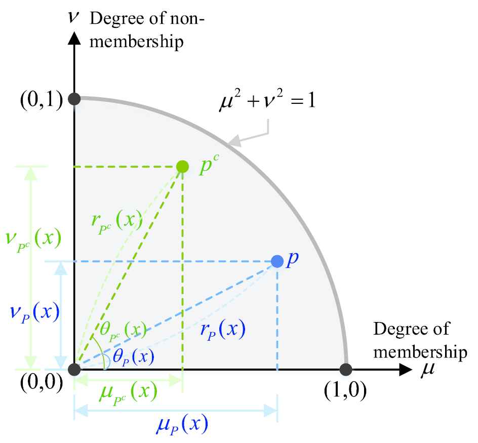
It is noted that the larger the value of
In particular, when
It is worthwhile to mention that the membership degree
Yager [19,20] employed the Takagi–Sugeno approach to propose a scalar function from fuzzy rule bases. Chen [33] indicated that Yager's scalar function can provide a representative value associated with each PF information and possess several useful and desirable properties. Liu and Zhang [27] investigated essential properties of Yager's function and studied some partial orders on Π−i numbers.
Definition 4.
[19,20,33] Let
Theorem 1.
For a PF set P, the PF scalar function V(p) of a Pythagorean membership grade
(T1.1)
(T1.2)
(T1.3)
(T1.4) V(p) decreases as
(T1.5) V(p) decreases as
(T1.6) V(p) increases as
(T1.7) V(p) is not a one-to-one mapping.
3. MCGDM PROBLEM UNDER PF UNCERTAINTY
This section intends to formulate an MCGDM problem under complex uncertainty of Pythagorean fizziness.
Consider an MCGDM problem based on PF sets. Let
Let
Let Pk denote the decision-maker ek's PF decision matrix in an MCGDM problem within the PF environment; Pk is concisely expressed as follows:
It is worth noting that the PF evaluative ratings can be conveniently acquired through the medium of applicable linguistic rating scales. Consider a nine-point rating scale as an example. Table 1 depicts some practical and beneficial approaches to evaluate the alternatives by use of nine-point linguistic scales. To be specific, Gündoǧdu [36] introduced a useful nine-point linguistic scale for facilitating the construction of the evaluation matrix based on PF sets and spherical fuzzy sets. Mete [37], Oz et al. [38], and Pérez-Domínguez et al. [39] employed an identical nine-point scale for expressing linguistic evaluations in PF settings. Rani et al. [40] introduced a nine-point linguistic scale for assisting decision-makers' judgments concerning the performance evaluations of alternatives in terms of criteria. Seker and Aydin [41] provided nine-point linguistic terms and their corresponding interval-valued PF numbers that can be used for the evaluation of alternatives with criteria. By applying a middle-point approach, these interval-valued PF numbers can be converted into Pythagorean membership grades, and the obtained results are shown in Table 1.
| Source | Linguistic Term | PF Evaluative Rating |
|---|---|---|
| Gündoǧdu [36] | Absolutely high | (0.90, 0.10; 0.91, 0.93) |
| Very high | (0.80, 0.20; 0.82, 0.84) | |
| High | (0.70, 0.30; 0.76, 0.74) | |
| Slightly high | (0.60, 0.40; 0.72, 0.63) | |
| Fair | (0.50, 0.50; 0.71, 0.50) | |
| Slightly low | (0.40, 0.60; 0.72, 0.37) | |
| Low | (0.30, 0.70; 0.76, 0.26) | |
| Very low | (0.20, 0.80; 0.82, 0.16) | |
| Absolutely low | (0.10, 0.90; 0.91, 0.07) | |
| Mete [37]; | Absolutely high | (1.00, 0.10; 1.00, 0.94) |
| Oz et al. [38]; | Very high | (0.80, 0.44; 0.91, 0.68) |
| Pérez-Domínguez [39] | High | (0.70, 0.60; 0.92, 0.55) |
| Moderately high | (0.60, 0.71; 0.93, 0.45) | |
| Medium | (0.50, 0.80; 0.94, 0.36) | |
| Moderately low | (0.40, 0.87; 0.96, 0.27) | |
| Low | (0.25, 0.92; 0.95, 0.17) | |
| Very low | (0.10, 0.97; 0.98, 0.07) | |
| Absolutely low | (0.10, 0.99; 1.00, 0.06) | |
| Rani et al. [40] | Absolutely high | (0.98, 0.20; 1.00, 0.87) |
| Very high | (0.87, 0.35; 0.94, 0.76) | |
| High | (0.70, 0.40; 0.81, 0.67) | |
| Medium high | (0.65, 0.45; 0.79, 0.61) | |
| Average | (0.50, 0.55; 0.74, 0.47) | |
| Medium low | (0.40, 0.70; 0.81, 0.33) | |
| Low | (0.36, 0.80; 0.88, 0.27) | |
| Very low | (0.25, 0.87; 0.91, 0.18) | |
| Very very low | (0.20, 0.98; 1.00, 0.13) | |
| Seker and | Absolutely good | (0.81, 0.10; 0.82, 0.92) |
| Aydin [41] | Very good | (0.72, 0.19; 0.74, 0.84) |
| Good | (0.63, 0.28; 0.69, 0.73) | |
| Medium good | (0.54, 0.37; 0.65, 0.62) | |
| Fair | (0.45, 0.45; 0.64, 0.50) | |
| Medium bad | (0.37, 0.54; 0.65, 0.38) | |
| Bad | (0.28, 0.63; 0.69, 0.27) | |
| Very bad | (0.19, 0.72; 0.74, 0.16) | |
| Absolutely bad | (0.10, 0.81; 0.82, 0.08) |
Pythagorean fuzzy (PF) evaluative ratings in relation to linguistic scales.
Decision-makers can express the linguistic evaluation values of alternatives toward each criterion. Afterward, these linguistic terms are transformed into PF evaluative ratings by the agency of the linguistic rating system in Table 1. Accordingly, the PF decision matrices from decision-makers can be determined using an appropriate linguistic rating system (e.g., the linguistic terms given in Table 1).
The decision-maker ek provides individual preference relations between the alternatives in the set Z with the preference set Ωk in which Ωk denotes a set of ordered pairs
Theoretically, the preference set Ωk contains at most
To deal with partial preference relations based on human subjective judgments, this paper devises a scheme that comes as close as possible to meet most of the decision-makers' paired preference relations in developing the PF LINMAP methods. In particular, this paper defines a useful synthetic index, named a comprehensive dominance measure, to evaluate the overall dominance of competing alternatives. The obtained overall dominance relations are contrasted with paired preference relations in the preference sets Ωk for all
4. DOMINANCE MEASURE VIA PF SCALAR FUNCTIONS
This section introduces different points of reference for PF information and establishes two types of PF scalar function-based dominance measures for facilitating intracriterion comparisons of PF evaluative ratings.
In general, different points of reference might have distinct influences on the contrast of various PF evaluative ratings, which would result in the change of the decision-makers' preference intensities. In this respect, this paper considers two types of reference points to define the PF scalar function-based dominance measures. First, the displaced reference points (i.e., the positive-ideal and negative-ideal reference points) under anchored judgments are utilized to construct the Type I dominance measure. Second, this paper regard the largest Pythagorean membership grade (1, 0; 1, 1) and the smallest grade (0, 1; 1, 0) as the fixed reference points for presenting the Type II dominance measure.
Definition 5.
(Displaced reference points) For each decision-maker ek's PF decision matrix
Definition 6.
(Fixed reference points) For each decision-maker ek, the largest fixed reference point
Based on Definition 2, the radians
Theorem 2.
The PF scalar function
(T2.1)
(T2.2)
(T2.3)
(T2.4)
(T2.5)
(T2.6)
(T2.7)
Proof.
(T2.1) is obvious from (T1.1). For the necessity of (T2.2), if
Note that
Definition 7.
Regarding a PF evaluative rating
The PF scalar function-based dominance measure of
Theorem 3.
The Type I dominance measure
(T3.1)
(T3.2) If
(T3.3) If
Proof.
For (T3.1), it is known that the PF scalar functions
Theorem 4.
The Type II dominance measure
(T4.1)
(T4.2) If
(T4.3) If
Proof.
The proofs of (T4.1)–(T4.3) are similar to those of (T3.1)–(T3.3), respectively.
Theorem 5.
The PF scalar function-based dominance measures
Proof.
From Definition 5, it is easily observed that
Theorem 6.
For two PF evaluative ratings
Proof.
According to a natural quasi-ordering on the space of Pythagorean membership grades [20,31],
As demonstrated in Theorems 3–6, the PF scalar function-based dominance measures
Definition 8.
Let
Theorem 7.
The Type I comprehensive dominance measure
(T7.1)
(T7.2) If
(T7.3) If
(T7.4) If
Proof.
For (T7.1), it is obvious that
Theorem 8.
The Type II comprehensive dominance measure
(T8.1)
(T8.2)
(T8.3) If
(T8.4) If
(T8.5) If
Proof.
(T8.1) can be easily checked based on Theorem 5. The proofs of (T8.2)–(T8.5) are analogous to those of (T7.1)–(T7.4), respectively.
5. PROPOSED PF LINMAP METHODOLOGY
This section utilizes the PF scalar function-based appoach to bring forward a novel PF LINMAP methodology. Moreover, two effective algorithmic procedures based on Types I and II dominance measures are also provided to facilitate solving MCGDM problems in PF contexts.
The proposed comprehensive dominance measures can be utilized to specify the overall dominance relations among candidate alternatives. Recall that the preference set Ωk is composed of the stated ordered pairs that represent the subjective preference relations between alternatives provided by the decision-maker ek. Based on the PF scalar function-based approach, this paper determines the overall dominance relations yielded by Type I or Type II comprehensive dominance measures. These results are contrasted with preference information provided by all decision-makers. More concretely, no error can be attributed to the paired preference relation between alternatives zϕ and zφ for the ordered pair
It is noteworthy that the decision-makers may indicate partial preference relations for the alternatives. Moreover, preference conflicts may exist among the decision-makers' subjective judgments. Accordingly, the comparison results between the stated subjective preferences and the overall dominance relations are somewhat conflicting. This paper employs the proposed comprehensive dominance measures to define the individual levels of rank consistency and rank inconsistency regarding the obtained overall dominance relations and the decision-maker's paired comparison judgments about alternatives. Based on the Type I comprehensive dominance measure, the individual level of rank consistency between the preorders of the alternatives zϕ and zφ for the ordered pair
Moreover, based on the Type II comprehensive dominance measure, the individual level of rank consistency for each
Note that
In contrast, this paper utilizes the Type I comprehensive dominance measure to define the individual level of rank inconsistency between the preorders of zϕ and zφ for each
Additionally, based on the Type II comprehensive dominance measure, the individual level of rank inconsistency for each
Note that
Next, this paper defines individual fit measurements for each decision-maker. This paper ascertains goodness of fit by integrating individual levels of rank consistency for all ordered pairs. Moreover, this paper figures out poorness of fit by combining individual levels of rank inconsistency. More specifically, for each decision-maker
It is worthy to note that
In the same way, this paper sums the individual levels of rank inconsistency
Because
In general, the decision-makers are conceived to prefer an alternative that has the highest group comprehensive dominance measure. Accordingly, it is reasonable to designate the total sum of group comprehensive dominance measures as a maximal objective. In particular, the total group comprehensive dominance measure is defined as the total sum of
In addition, it is reasonable to presume that the decision-maker ek would like to acquire a solution with a higher individual goodness of fit
Based on Type I dominance measures, to maximize the total group comprehensive dominance measure
Based on Type II dominance measures, the bi-objective (i.e., maximizing the
It is worth mentioning that the relative importance among multiple decision-makers can be appropriately reflected by means of the lowest acceptable level concerning the deviation between individual goodness of fit and individual poorness of fit. For example, if the importance of the decision-maker ek is higher than the other decision-makers, a relatively high
Let
It is easy to see that the following conditions hold:
Furthermore, the group poorness of fit
The differences
From Definition 8, one has
The bi-objective models in Models 2(I) and 2(II) can be further transformed into simple linear programming models for enhancing implementation efficiency. The minimal objectives
The optimal solutions of the collective weight
Lastly, the overall priority ranking results of candidate alternatives is acquired in conformity with the decreasing order of the values of
Based on Types I and II dominance measures, the algorithmic procedures of the proposed PF LINMAP methodology can be summarized as follows:
Algorithm I: Type I PF LINMAP method
Step I.1: Formulate an MCGDM problem involving the set of alternatives
Step I.2: Request each decision-maker ek to provide the paired preference relations over alternatives to form the preference set
Step I.3: Establish the PF evaluative rating
Step I.4: Identify the displaced reference points, i.e., the positive-ideal reference point
Step I.5: Derive the PF scalar function
Step I.6: Compute the PF scalar function-based dominance measure when anchoring
Step I.7: Set the parameter values. Specify the lowest acceptable level
Step I.8: Denote
Step I.9: Construct the linear programming problem using the Type I PF LINMAP model to resolve the optimal collective weight
Step I.10: Obtain the optimal group comprehensive dominance measure
6. PRACTICAL APPLICATION
This section employs the PF LINMAP techniques to address an MCGDM problem concerning railway project investment introduced by Xue et al. [26] to validate the practicability and effectiveness of the developed methodology in realistic situations.
Algorithm II: Type II PF LINMAP method
Steps II.1–II.3: see Steps I.1–I.3 of Algorithm I.
Step II.4: Calculate the PF scalar function
Step II.5: See Step I.7 of Algorithm I.
Step II.6: Denote
Step II.7: Construct the linear programming problem using the Type II PF LINMAP model to resolve the optimal collective weight
Step II.8: Obtain the optimal group comprehensive dominance measure
Xue et al. [26] utilized PF entropy measures to develop a novel PF LINMAP method and applied it to manage an MCGDM problem regarding the railway project selection in China's Belt and Road Initiative (BRI). Till now, BRI involves infrastructure development and investments in countries and international organizations in Asia, Europe, Africa, the Middle East, and the Americas. Consider the importance of railway projects in the infrastructure investment of BRI, Xue et al. took Germany (z1), Russia (z2), Singapore (z3), and Malaysia (z4) as the candidate alternatives in the set Z, because these countries have intentions to cooperate with the railway project. Moreover, Xue et al. explored an indicator system involving financial and noneconomic evaluations. Their proposed indicator system involves six aspects consisting of financial internal rate of return (c1), net present value (c2), investment recovery period (c3), debt ratio and current ratio (c4), repayment period of loan (c5), and public benefit and diplomatic influence (c6). The six aspects were regarded as the evaluative criteria in the set C. Three experts participated in a group decision-making process in this case. On the basis of the above, in Steps I.1 and II.1, the MCGDM problem under study was formulated with
First, this paper employed the proposed Algorithm I (i.e., Type I PF LINMAP method) to solve the above MCGDM problem. In Step I.2, in reference to the investigated data in Xue et al. [26], the three decision-makers provided some paired preference relations over alternatives. The decision-makers' preference sets were constructed as follows:
In Step I.3, the three decision-makers evaluated the four alternatives based on the six criteria; they provided the results of the degree of satisfaction
| zi | cj | ||||||
|---|---|---|---|---|---|---|---|
| z1 | c1 | 0.70 | 0.60 | 0.9220 | 0.5489 | 0.7086 | 0.5451 |
| c2 | 0.80 | 0.60 | 1.0000 | 0.5903 | 0.6435 | 0.5903 | |
| c3 | 0.50 | 0.50 | 0.7071 | 0.5000 | 0.7854 | 0.5000 | |
| c4 | 0.40 | 0.70 | 0.8062 | 0.3305 | 1.0517 | 0.3633 | |
| c5 | 0.90 | 0.40 | 0.9849 | 0.7338 | 0.4182 | 0.7302 | |
| c6 | 0.40 | 0.90 | 0.9849 | 0.2662 | 1.1526 | 0.2698 | |
| z2 | c1 | 0.90 | 0.40 | 0.9849 | 0.7338 | 0.4182 | 0.7302 |
| c2 | 0.80 | 0.60 | 1.0000 | 0.5903 | 0.6435 | 0.5903 | |
| c3 | 0.70 | 0.70 | 0.9899 | 0.5000 | 0.7854 | 0.5000 | |
| c4 | 0.90 | 0.30 | 0.9487 | 0.7952 | 0.3218 | 0.7800 | |
| c5 | 0.80 | 0.20 | 0.8246 | 0.8440 | 0.2450 | 0.7837 | |
| c6 | 0.90 | 0.40 | 0.9849 | 0.7338 | 0.4182 | 0.7302 | |
| z3 | c1 | 0.70 | 0.50 | 0.8602 | 0.6051 | 0.6202 | 0.5904 |
| c2 | 0.40 | 0.30 | 0.5000 | 0.5903 | 0.6435 | 0.5452 | |
| c3 | 0.90 | 0.10 | 0.9055 | 0.9296 | 0.1107 | 0.8890 | |
| c4 | 0.80 | 0.20 | 0.8246 | 0.8440 | 0.2450 | 0.7837 | |
| c5 | 0.70 | 0.40 | 0.8062 | 0.6695 | 0.5191 | 0.6367 | |
| c6 | 0.60 | 0.60 | 0.8485 | 0.5000 | 0.7854 | 0.5000 | |
| z4 | c1 | 0.90 | 0.30 | 0.9487 | 0.7952 | 0.3218 | 0.7800 |
| c2 | 0.70 | 0.20 | 0.7280 | 0.8228 | 0.2783 | 0.7350 | |
| c3 | 0.40 | 0.30 | 0.5000 | 0.5903 | 0.6435 | 0.5452 | |
| c4 | 0.90 | 0.40 | 0.9849 | 0.7338 | 0.4182 | 0.7302 | |
| c5 | 0.50 | 0.40 | 0.6403 | 0.5704 | 0.6747 | 0.5451 | |
| c6 | 0.60 | 0.70 | 0.9220 | 0.4511 | 0.8622 | 0.4549 |
Relevant data associated with the decision-maker e1.
| zi | cj | ||||||
|---|---|---|---|---|---|---|---|
| z1 | c1 | 0.50 | 0.40 | 0.6403 | 0.5704 | 0.6747 | 0.5451 |
| c2 | 0.30 | 0.90 | 0.9487 | 0.2048 | 1.2490 | 0.2200 | |
| c3 | 0.40 | 0.30 | 0.5000 | 0.5903 | 0.6435 | 0.5452 | |
| c4 | 0.90 | 0.40 | 0.9849 | 0.7338 | 0.4182 | 0.7302 | |
| c5 | 0.30 | 0.70 | 0.7616 | 0.2578 | 1.1659 | 0.3155 | |
| c6 | 0.40 | 0.50 | 0.6403 | 0.4296 | 0.8961 | 0.4549 | |
| z2 | c1 | 0.90 | 0.30 | 0.9487 | 0.7952 | 0.3218 | 0.7800 |
| c2 | 0.80 | 0.50 | 0.9434 | 0.6444 | 0.5586 | 0.6362 | |
| c3 | 0.70 | 0.60 | 0.9220 | 0.5489 | 0.7086 | 0.5451 | |
| c4 | 0.90 | 0.20 | 0.9220 | 0.8608 | 0.2187 | 0.8326 | |
| c5 | 0.90 | 0.20 | 0.9220 | 0.8608 | 0.2187 | 0.8326 | |
| c6 | 0.80 | 0.30 | 0.8544 | 0.7716 | 0.3588 | 0.7321 | |
| z3 | c1 | 0.70 | 0.60 | 0.9220 | 0.5489 | 0.7086 | 0.5451 |
| c2 | 0.50 | 0.30 | 0.5831 | 0.6560 | 0.5404 | 0.5909 | |
| c3 | 0.80 | 0.10 | 0.8062 | 0.9208 | 0.1244 | 0.8393 | |
| c4 | 0.90 | 0.10 | 0.9055 | 0.9296 | 0.1107 | 0.8890 | |
| c5 | 0.70 | 0.30 | 0.7616 | 0.7422 | 0.4049 | 0.6845 | |
| c6 | 0.50 | 0.50 | 0.7071 | 0.5000 | 0.7854 | 0.5000 | |
| z4 | c1 | 0.30 | 0.90 | 0.9487 | 0.2048 | 1.2490 | 0.2200 |
| c2 | 0.20 | 0.30 | 0.3606 | 0.3743 | 0.9828 | 0.4547 | |
| c3 | 0.30 | 0.70 | 0.7616 | 0.2578 | 1.1659 | 0.3155 | |
| c4 | 0.50 | 0.80 | 0.9434 | 0.3556 | 1.0122 | 0.3638 | |
| c5 | 0.70 | 0.60 | 0.9220 | 0.5489 | 0.7086 | 0.5451 | |
| c6 | 0.40 | 0.70 | 0.8062 | 0.3305 | 1.0517 | 0.3633 |
Relevant data associated with the decision-maker e2.
| zi | cj | ||||||
|---|---|---|---|---|---|---|---|
| z1 | c1 | 0.40 | 0.30 | 0.5000 | 0.5903 | 0.6435 | 0.5452 |
| c2 | 0.30 | 0.40 | 0.5000 | 0.4097 | 0.9273 | 0.4548 | |
| c3 | 0.50 | 0.40 | 0.6403 | 0.5704 | 0.6747 | 0.5451 | |
| c4 | 0.60 | 0.60 | 0.8485 | 0.5000 | 0.7854 | 0.5000 | |
| c5 | 0.70 | 0.70 | 0.9899 | 0.5000 | 0.7854 | 0.5000 | |
| c6 | 0.30 | 0.70 | 0.7616 | 0.2578 | 1.1659 | 0.3155 | |
| z2 | c1 | 0.80 | 0.30 | 0.8544 | 0.7716 | 0.3588 | 0.7321 |
| c2 | 0.70 | 0.10 | 0.7071 | 0.9097 | 0.1419 | 0.7897 | |
| c3 | 0.80 | 0.20 | 0.8246 | 0.8440 | 0.2450 | 0.7837 | |
| c4 | 0.90 | 0.10 | 0.9055 | 0.9296 | 0.1107 | 0.8890 | |
| c5 | 0.80 | 0.30 | 0.8544 | 0.7716 | 0.3588 | 0.7321 | |
| c6 | 0.80 | 0.10 | 0.8062 | 0.9208 | 0.1244 | 0.8393 | |
| z3 | c1 | 0.20 | 0.50 | 0.5385 | 0.2422 | 1.1903 | 0.3612 |
| c2 | 0.30 | 0.40 | 0.5000 | 0.4097 | 0.9273 | 0.4548 | |
| c3 | 0.80 | 0.60 | 1.0000 | 0.5903 | 0.6435 | 0.5903 | |
| c4 | 0.90 | 0.10 | 0.9055 | 0.9296 | 0.1107 | 0.8890 | |
| c5 | 0.30 | 0.10 | 0.3162 | 0.7952 | 0.3218 | 0.5933 | |
| c6 | 0.60 | 0.40 | 0.7211 | 0.6257 | 0.5880 | 0.5906 | |
| z4 | c1 | 0.60 | 0.80 | 1.0000 | 0.4097 | 0.9273 | 0.4097 |
| c2 | 0.40 | 0.10 | 0.4123 | 0.8440 | 0.2450 | 0.6419 | |
| c3 | 0.20 | 0.40 | 0.4472 | 0.2952 | 1.1071 | 0.4084 | |
| c4 | 0.70 | 0.10 | 0.7071 | 0.9097 | 0.1419 | 0.7897 | |
| c5 | 0.60 | 0.20 | 0.6325 | 0.7952 | 0.3218 | 0.6867 | |
| c6 | 0.80 | 0.10 | 0.8062 | 0.9208 | 0.1244 | 0.8393 |
Relevant data associated with the decision-maker e3.
In Step I.4, this paper employed Eqs. (14) and (15) to identify the displaced reference points
| ek | cj | ||||||
|---|---|---|---|---|---|---|---|
| e1 | c1 | 0.90 | 0.30 | 0.9487 | 0.7952 | 0.3218 | 0.7800 |
| c2 | 0.80 | 0.20 | 0.8246 | 0.8440 | 0.2450 | 0.7837 | |
| c3 | 0.90 | 0.10 | 0.9055 | 0.9296 | 0.1107 | 0.8890 | |
| c4 | 0.90 | 0.20 | 0.9220 | 0.8608 | 0.2187 | 0.8326 | |
| c5 | 0.90 | 0.20 | 0.9220 | 0.8608 | 0.2187 | 0.8326 | |
| c6 | 0.90 | 0.40 | 0.9849 | 0.7338 | 0.4182 | 0.7302 | |
| e2 | c1 | 0.90 | 0.30 | 0.9487 | 0.7952 | 0.3218 | 0.7800 |
| c2 | 0.80 | 0.30 | 0.8544 | 0.7716 | 0.3588 | 0.7321 | |
| c3 | 0.80 | 0.10 | 0.8062 | 0.9208 | 0.1244 | 0.8393 | |
| c4 | 0.90 | 0.10 | 0.9055 | 0.9296 | 0.1107 | 0.8890 | |
| c5 | 0.90 | 0.20 | 0.9220 | 0.8608 | 0.2187 | 0.8326 | |
| c6 | 0.80 | 0.30 | 0.8544 | 0.7716 | 0.3588 | 0.7321 | |
| e3 | c1 | 0.80 | 0.30 | 0.8544 | 0.7716 | 0.3588 | 0.7321 |
| c2 | 0.70 | 0.10 | 0.7071 | 0.9097 | 0.1419 | 0.7897 | |
| c3 | 0.80 | 0.20 | 0.8246 | 0.8440 | 0.2450 | 0.7837 | |
| c4 | 0.90 | 0.10 | 0.9055 | 0.9296 | 0.1107 | 0.8890 | |
| c5 | 0.80 | 0.10 | 0.8062 | 0.9208 | 0.1244 | 0.8393 | |
| c6 | 0.80 | 0.10 | 0.8062 | 0.9208 | 0.1244 | 0.8393 |
Results of the positive-ideal reference point
| ek | cj | ||||||
|---|---|---|---|---|---|---|---|
| e1 | c1 | 0.70 | 0.60 | 0.9220 | 0.5489 | 0.7086 | 0.5451 |
| c2 | 0.40 | 0.60 | 0.7211 | 0.3743 | 0.9828 | 0.4094 | |
| c3 | 0.40 | 0.70 | 0.8062 | 0.3305 | 1.0517 | 0.3633 | |
| c4 | 0.40 | 0.70 | 0.8062 | 0.3305 | 1.0517 | 0.3633 | |
| c5 | 0.50 | 0.40 | 0.6403 | 0.5704 | 0.6747 | 0.5451 | |
| c6 | 0.40 | 0.90 | 0.9849 | 0.2662 | 1.1526 | 0.2698 | |
| e2 | c1 | 0.30 | 0.90 | 0.9487 | 0.2048 | 1.2490 | 0.2200 |
| c2 | 0.20 | 0.90 | 0.9220 | 0.1392 | 1.3521 | 0.1674 | |
| c3 | 0.30 | 0.70 | 0.7616 | 0.2578 | 1.1659 | 0.3155 | |
| c4 | 0.50 | 0.80 | 0.9434 | 0.3556 | 1.0122 | 0.3638 | |
| c5 | 0.30 | 0.70 | 0.7616 | 0.2578 | 1.1659 | 0.3155 | |
| c6 | 0.40 | 0.70 | 0.8062 | 0.3305 | 1.0517 | 0.3633 | |
| e3 | c1 | 0.20 | 0.80 | 0.8246 | 0.1560 | 1.3258 | 0.2163 |
| c2 | 0.30 | 0.40 | 0.5000 | 0.4097 | 0.9273 | 0.4548 | |
| c3 | 0.20 | 0.60 | 0.6325 | 0.2048 | 1.2490 | 0.3133 | |
| c4 | 0.60 | 0.60 | 0.8485 | 0.5000 | 0.7854 | 0.5000 | |
| c5 | 0.30 | 0.70 | 0.7616 | 0.2578 | 1.1659 | 0.3155 | |
| c6 | 0.30 | 0.70 | 0.7616 | 0.2578 | 1.1659 | 0.3155 |
Results of the negative-ideal reference point
In Step I.5, this paper utilized Eq. (18) to compute the PF scalar functions
In Step I.6, this paper employed the PF scalar functions
| ek | cj | ||||
|---|---|---|---|---|---|
| e1 | c1 | 0.0000 | 0.7880 | 0.1931 | 1.0000 |
| c2 | 0.4834 | 0.4834 | 0.3628 | 0.8699 | |
| c3 | 0.2600 | 0.2600 | 1.0000 | 0.3459 | |
| c4 | 0.0000 | 0.8879 | 0.8957 | 0.7818 | |
| c5 | 0.6438 | 0.8298 | 0.3184 | 0.0000 | |
| c6 | 0.0000 | 1.0000 | 0.5000 | 0.4021 | |
| e2 | c1 | 0.5805 | 1.0000 | 0.5805 | 0.0000 |
| c2 | 0.0932 | 0.8303 | 0.7501 | 0.5088 | |
| c3 | 0.4385 | 0.4383 | 1.0000 | 0.0000 | |
| c4 | 0.6977 | 0.8927 | 1.0000 | 0.0000 | |
| c5 | 0.0000 | 1.0000 | 0.7135 | 0.4439 | |
| c6 | 0.2483 | 1.0000 | 0.3706 | 0.0000 | |
| e3 | c1 | 0.6376 | 1.0000 | 0.2809 | 0.3749 |
| c2 | 0.0000 | 1.0000 | 0.0000 | 0.5585 | |
| c3 | 0.4928 | 1.0000 | 0.5889 | 0.2021 | |
| c4 | 0.0000 | 1.0000 | 1.0000 | 0.7447 | |
| c5 | 0.3522 | 0.7953 | 0.5304 | 0.7086 | |
| c6 | 0.0000 | 1.0000 | 0.5252 | 1.0000 |
Results of the Type I dominance measure
In Step I.7, this paper regarded the three decision-makers of equal importance to designate the lowest acceptable level
In Step I.8, let
In Step I.9, this paper applied the Type I PF LINMAP model in Eq. (47) to construct a parametric linear programming model, as shown in the Appendix. The model was solved to obtain the optimal collective weight vector and individual degrees of violation as follows:
In Step I.10, the optimal group comprehensive dominance measures were derived using Eq. (49) as follows:
Next, this paper employed the developed Algorithm II (i.e., Type II PF LINMAP method) to handle the above MCGDM problem. It is noted that Steps II.1–II.3 and II.5 of Algorithm II are the same as Steps I.1–I.3 and I.7 of Algorithm I, respectively.
In Step II.4, this paper computed the PF scalar function
In Step II.6, let the weight vector of criteria
In Step II.7, this paper employed the Type II PF LINMAP model in Eq. (48) to set up a parametric linear programming model. Solving the model, the optimal collective weight vector
In Step II.8, the optimal group comprehensive dominance measures were obtained using Eq. (50) as follows:
7. COMPARATIVE ANALYSIS AND DISCUSSIONS
This section intends to implement a sensitivity analysis and conduct some comparative studies to validate the workableness and attractiveness of the proposed methodology.
Based on the Types I and II PF LINMAP models in Eqs. (47) and (48), the parameter η can adjust the proportion of the “total group comprehensive dominance” part and the “group poorness of fit” part. The proposed methodology, which originate from classical LINMAP, should initiate ideas that are least violated in regard to the decision-makers' paired preference relations over alternatives. This implies that the proportion of the “group poorness of fit” part (with the weight
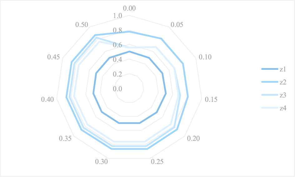
The first sensitivity analysis investigates the influences of various values of the parameter η on the solution results using the Type I PF LINMAP model. Consider eleven cases in which

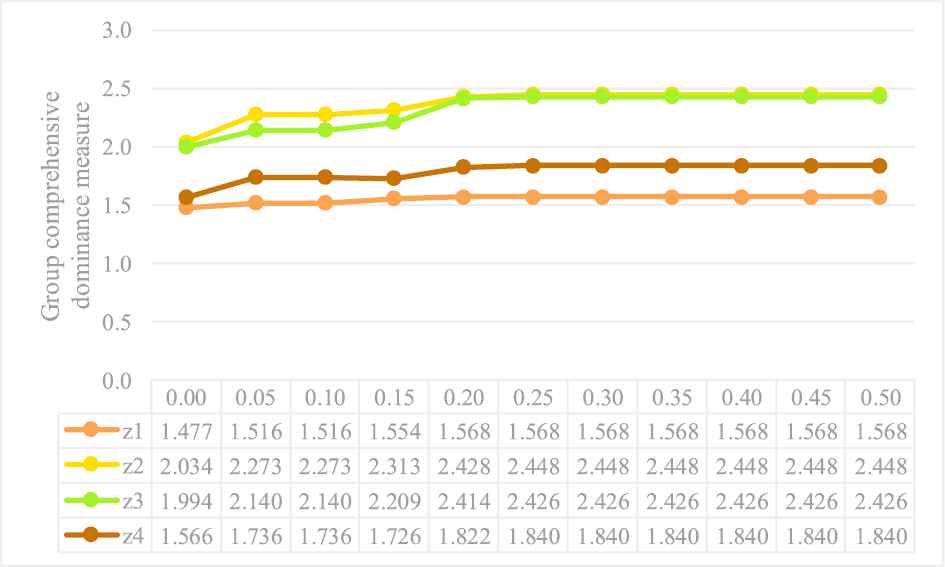
Comparisons of the optimal group comprehensive dominance measure
According to the comparison results in Figure 2, it is easy to observe that the Type I PF LINMAP model has high robustness because the identical ranking results were obtained in most cases. As shown in this figure, the Type I PF LINMAP model rendered the overall priority ranking
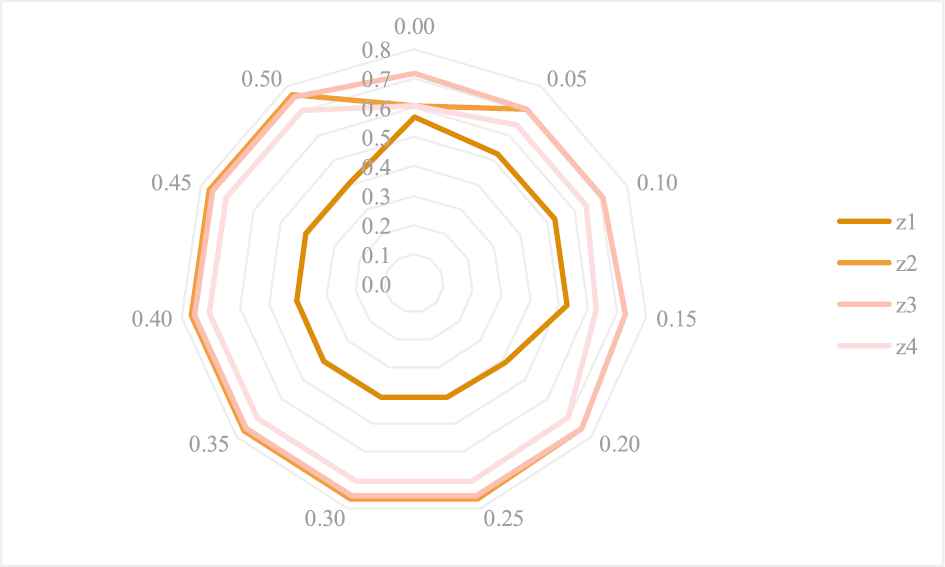
Additionally, the contrast results of the optimal Type I comprehensive dominance measure
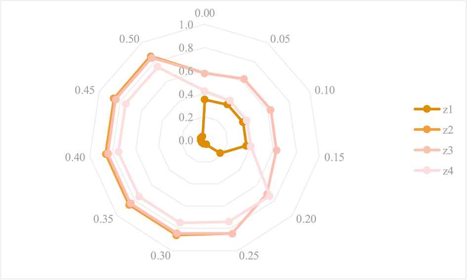
Contrasts of the optimal Type I comprehensive dominance measure
Contrasts of the optimal Type I comprehensive dominance measure
Contrasts of the optimal Type I comprehensive dominance measure
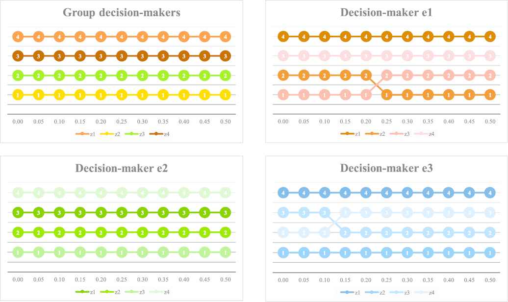
The priority rankings of the four alternatives rendered by the Type I PF LINMAP model are demonstrated in Figure 6, consisting of the overall priority ranking orders for group decision-makers and the individual ranking orders for each decision-maker. As mentioned before, the overall priority ranking
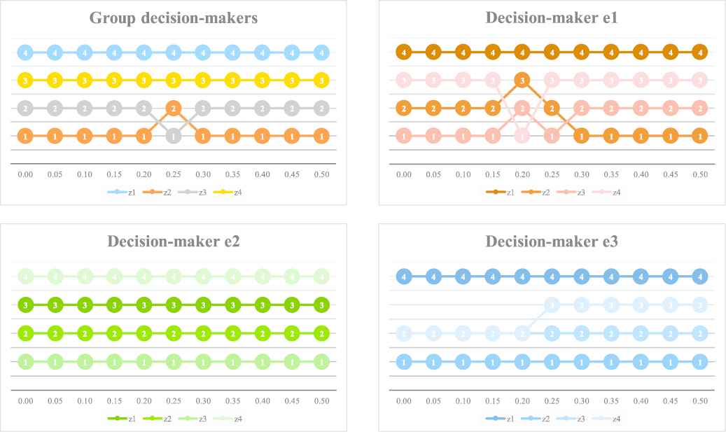
Results of the priority ranking orders for group and individual decision-makers via the Type I PF linear programming technique for multidimensional analysis of preference (LINMAP) model.
The second sensitivity analysis explores the effects of different values of the parameter η on the results using the Type II PF LINMAP model. Let
Comparisons of the optimal group comprehensive dominance measure
From Figure 7, it can be observed that the Type II PF LINMAP model shows strong robustness because the same ranking results were obtained in all of the investigated cases. Specifically, the Type II PF LINMAP model produced the overall priority ranking
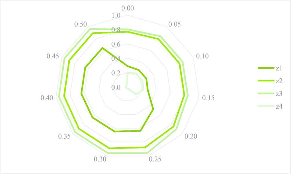
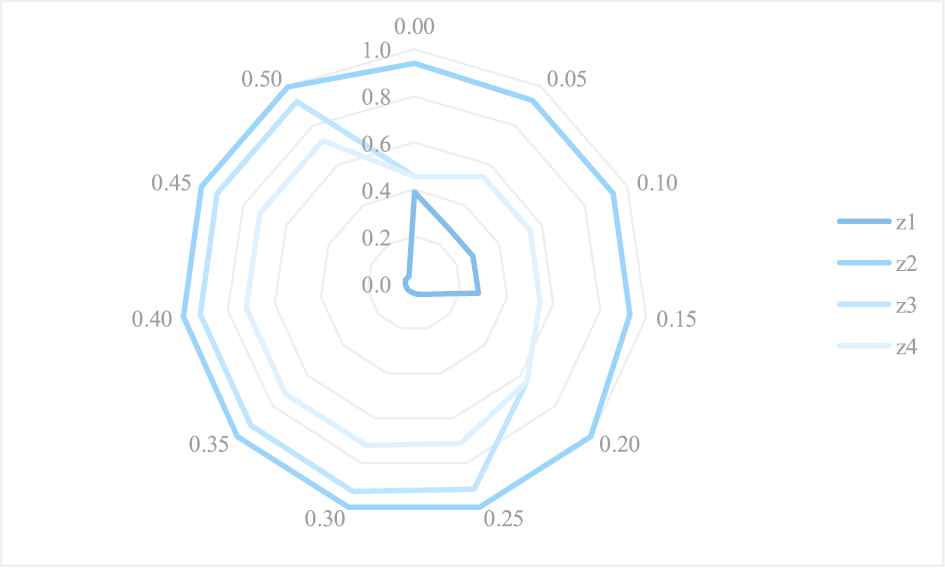
The comparison results of the optimal Type II comprehensive dominance measure
Contrasts of the optimal Type II comprehensive dominance measure
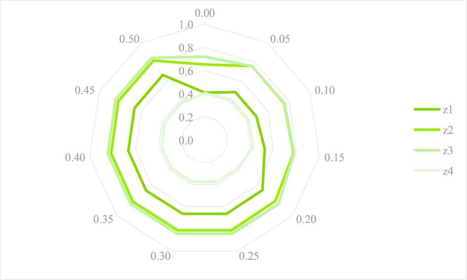
Contrasts of the optimal Type II comprehensive dominance measure
Contrasts of the optimal Type II comprehensive dominance measure
Figure 11 shows the ranking results of the four candidate alternatives produced by the Type II PF LINMAP model. The graphs in this figure consist of the overall priority ranking orders for group decision-makers and the individual ranking orders for each decision-maker. In line with Figure 7, the overall priority ranking
Results of the priority ranking orders for group and individual decision-makers via the Type II PF linear programming technique for multidimensional analysis of preference (LINMAP) model.
Xue et al. [26] conducted a comprehensive analysis on the MCGDM problem involving the railway project investment to show the reliability and the sensitivity of their developed PF entropy-based LINMAP method. The three rankings
8. CONCLUSIONS
This paper has extended the core structure of the classical LINMAP methods to the complex uncertainty of Pythagorean fuzziness and has developed a new PF LINMAP-based compromising methodology based on the proposed PF scalar function-based approach for solving MCGDM problems.
The proposed PF LINMAP methodology not only has the merit of the LINMAP in handling preference information over alternatives but also enhance uncertain LINMAP-based approaches by incorporating some novel concepts (e.g., PF scalar function-based dominance measures and Types I and II comprehensive dominance measures) in the core procedure of LINMAP. Two parametric linear programming problems have been formulated for effectively implementing Types I and II PF LINMAP models. Moreover, compared with the Type I PF LINMAP model, the Type II PF LINMAP model has the merits of simplicity and efficiency. The helpfulness and effectiveness of the proposed PF LINMAP-based compromising methods have been verified via the application to the MCGDM problem in regard to railway project investment. Compared to the existing PF LINMAP methods, the developed PF scalar function-based approach is capable of manipulating PF information in a fairly easy and straightforward matter. Moreover, both Types I and II PF LINMAP models have high robustness because of the reasonable and reliable application results via the sensitivity analysis and discussions. Future research can focus on the extension of incorporating the PF scalar function-based approach into other decision-making models. Furthermore, the proposed PF LINMAP-based compromising methodology can be applied to address uncertain MCGDM problems in other application fields.
CONFLICT OF INTEREST
The authors declare that there is no conflict of interest regarding the publication of this paper.
AUTHORS' CONTRIBUTIONS
Jih-Chang Wang: Methodology, Software, Validation, Formal analysis, Data Curation, Writing – Original Draft, Visualization. Ting-Yu Chen: Conceptualization, Methodology, Validation, Formal analysis, Writing – Original Draft, Writing – Review & Editing, Supervision, Funding acquisition.
DATA AVAILABILITY STATEMENT
The datasets generated during and/or analyzed during the current study are available from the corresponding author on reasonable request.
ETHICAL APPROVAL
This article does not contain any studies with human participants or animals that were performed by the authors.
ACKNOWLEDGMENTS
The authors acknowledge the assistance of the respected editor and the anonymous referees for their insightful and constructive comments, which helped to improve the overall quality of the paper. The corresponding author Ting-Yu Chen is grateful for grant funding support from the Taiwan Ministry of Science and Technology (MOST 108-2410-H-182-014-MY2) and Chang Gung Memorial Hospital (BMRP 574 and CMRPD2F0203) during the completion of this study.
APPENDIX
REFERENCES
Cite this article
TY  - JOUR
AU  - Jih-Chang Wang
AU  - Ting-Yu Chen
PY  - 2020
DA  - 2020/04/23
TI  - A Novel Pythagorean Fuzzy LINMAP-Based Compromising Approach for Multiple Criteria Group Decision-Making with Preference Over Alternatives
JO  - International Journal of Computational Intelligence Systems
SP  - 444
EP  - 463
VL  - 13
IS  - 1
SN  - 1875-6883
UR  - https://doi.org/10.2991/ijcis.d.200408.001
DO  - 10.2991/ijcis.d.200408.001
ID  - Wang2020
ER  -