
Enhancing of Artificial Bee Colony Algorithm for Virtual Machine Scheduling and Load Balancing Problem in Cloud Computing
- DOI
- 10.2991/ijcis.d.200410.002How to use a DOI?
- Keywords
- Artificial bee colony algorithm; Cloud computing; Scheduling algorithms; Load balance; Resource management; Distribution
- Abstract
This paper proposes the combination of Swarm Intelligence algorithm of artificial bee colony with heuristic scheduling algorithm, called Heuristic Task Scheduling with Artificial Bee Colony (HABC). This algorithm is applied to improve virtual machines scheduling solution for cloud computing within homogeneous and heterogeneous environments. It was introduced to minimize makespan and balance the loads. The scheduling performance of the cloud computing system with HABC was compared to that supplemented with other swarm intelligence algorithms: Ant Colony Optimization (ACO) with standard heuristic algorithm, Particle Swarm Optimization (PSO) with standard heuristic algorithm and improved PSO (IPSO) with standard heuristic algorithm. In our experiments, CloudSim was used to simulate systems that used different supplementing algorithms for the purpose of comparing their makespan and load balancing capability. The experimental results can be concluded that virtual machine scheduling management with artificial bee colony algorithm and largest job first (HABC_LJF) outperformed those with ACO, PSO, and IPSO.
- Copyright
- © 2020 The Authors. Published by Atlantis Press SARL.
- Open Access
- This is an open access article distributed under the CC BY-NC 4.0 license (http://creativecommons.org/licenses/by-nc/4.0/).
1. INTRODUCTION
Artificial Bee Colony (ABC) is a Swarm Intelligent (SI) algorithm inspired by the foraging behavior of honey bees proposed by Karaboga in 2005 [1,2] and it is modified from Bee Colony Optimization (BCO) that was proposed for the first time in 2001 [3]. The foraging habits of honey bees are foraging and waggle dancing. The main idea is to create the multi agent system which is the colony of artificial bees to be able to efficiently solve hard combinatorial optimization problems. Therefore, ABC has been successfully employed in optimizations problems like data-mining problem [4,5], job shop scheduling [6,7], binary optimization [8–10], travelling salesman [11], biochemical networks [12], engineering optimization [13,14], image processing [15–17], as well as scheduling problem in cloud computing [18–21].
Cloud computing system [22,23] provides computing services via the Internet which will be operated upon user's requests. The requests are to manage the resources and services used through the system software. The user can control the amount of resources used such as CPU or RAM to an extent without having knowledge about the service types [24]. As cloud computing is based on virtualization technology that has no restriction on computing resources, it has a great advantage for service providers in terms of simplicity, energy saving, and low resource management cost. Cloud computing uses a virtualization technique to create Virtual Machines (VMs) [25,26]. It uses software to make a computer work like a system of multiple computers (VMs). VMs can replace a physical computer server and other necessary physical resources as they have their own independent virtual resources [27].
Tasks scheduling is a challenging problem and known to be NP-complete problem [28,29]. If the same server is simultaneously being requested to be used by many users, the other servers will become idle. This is called load imbalance. This problem can be solved by an algorithm to schedule tasks properly prior to service processing on VMs. A system with a proper task scheduling algorithm can also provide an advantage of efficient use of the system resources, i.e., it can reduce waiting time for a service queue and distribute some tasks to other servers. The implementation of this algorithm is called load balancing.
The operations of cloud computing are quite similar to those of ABC algorithm as both can adapt themselves to their environment which is a characteristic of the foraging behavior of bees. Their objectives are also similar: the objective of cloud computing is to maximize throughput for a desired makespan while that of bee foraging behavior is to find a food source with a large amount of honey with the least amount of effort.
The main contributions of this paper are to propose the idea of applying ABC algorithm and a task scheduling heuristic to each VM. The algorithm will minimize the makespan or the overall processing time of tasks and provide load balancing in cloud computing. Moreover, we focused on cloud computing within both homogeneous and heterogeneous environments and observed how good the HABC algorithm works when the number of tasks in the system was varied and the type of datasets was changed. It is found that this algorithm performed the task scheduling better than ACO, PSO, and IPSO.
The paper is structured as follows: the related works, including task scheduling and load balancing in cloud computing and the ABC algorithm are described in Section 2. Adoption of a scheduling heuristic and load balancing algorithm inspired by ABC for cloud computing is proposed in Section 3. The experimental settings and results are discussed in Section 4. Finally, Section 5 presents the conclusion.
2. BACKGROUND AND RELATED WORK
2.1. Task Scheduling and Load Balancing in Cloud Computing
Cloud computing system creates a shared network resource and service with the user. Due to its diversified, dynamic, and flexible nature, different resources and services offering to different users, are the advantages of cloud computing. It provides a service upon user's request [24,30]. Cloud service providers offer various cloud services to user [22,23]. Resource management in cloud computing varies depending on the kind of user's request.
Heterogeneity in cloud computing depends on the infrastructure and service provided by providers. In case of providing the system with the same infrastructure to software packages and resources, the environment in the system will be called homogeneous cloud environment [31], while the environment in a system with different resources are provided by different providers, software packages by some other, infrastructure by yet another will be called heterogeneous cloud environment [32].
Over the last few years, exhaustive researchers have proposed several different task scheduling algorithms which run under the cloud computing resource utilization. Task scheduling algorithms mostly aimed to balance the workload that users requested for within the limitation of the system resources and to increase the efficiency of cloud computing. For example, Chase et al. [33] presented implementation of an architecture for resource management for large server clusters in order to provision server resources for co-hosted services and improve the energy efficiency of server clusters by dynamically resizing the active server set.
In 2009, D. Kusic et al. [34] presented a lookahead control scheme to solve a dynamic resource provisioning framework for a multi-objective optimization in a virtualized server environment. The technique can approach accounts for the switching costs incurred while provisioning VMs and explicitly encodes the corresponding risk in the optimization problem.
In 2011, D. Minarolli and B. Freisleben [35], proposed a scheme that dynamically allocates the resources to VMs. Such that quality of service constraints is satisfied, and its operating costs are minimized by a two-tier resource management approach based on adequate utility functions. Later in 2012, A. Gorbenko and V. Popov [36] proposed a logical model to solve the task-resource scheduling problem that minimized the resource and cost by applying algorithms for the satisfiability problem (SAT).
In 2013, S. Son et al. [37] proposed a Service Level Agreement (SLA) based on cloud computing framework to facilitate resource allocation considering the workload and geographical location of distributed data centers. This approach was suggested to tackle using the automated SLA negotiation mechanism and a Workload and Location-aware Resource Allocation scheme (WLARA) supports providers in earning higher profits. In 2015, A. Singh and K. Dutta [38], presented the resource allocation algorithm by Analytic Hierarchy Process (AHP) with a pairwise comparison matrix technique. This proposed technique made a better resource allocation than other algorithms. In 2017, Ullah et al. [39] presented a real-time resource usage prediction system which took real-time utilization of resources and fed utilization values into several buffers based on the resource types and time span size. Scheduling problem have been also discussed in different contents as in Refs. [40–42].
2.2. Related Work about Bioinspired and Meta-Heuristics Algorithms to Solve Cloud Computing
The nature-inspired metaheuristics algorithms attempt to attain the global optimal solution by examining the most suitable locations in the search space domain, based on the natural mechanism. The methods are different depending on type of algorithms, because some algorithms are suitable in solving specific type of problems but not suitable for others. This is due to the randomization or stochastic strategies that are used in solving those NP-Hard problems.
There are many previous works had proposed many metaheuristic-based approaches to scheduling workflow applications [43]. In particular, Genetic Algorithms (GA) [44,45], Particle Swarm Optimization (PSO) algorithms [46–49], Cuckoo Search (CS) algorithm [50–54], and Ant Colony Optimization (ACO) algorithm [55–56] have been used for scheduling workflows. For instance, Dasgupta et al. [45] proposed GA which is a balance the load of the cloud and minimizing the make span of a given tasks set. In 2010, S. Pandey et al. [46] proposed a PSO based heuristic to schedule applications to cloud resources that considers both computation cost and data transmission cost.
In 2019, H. Saleh et al. [49] proposed a cloud task scheduling with improved PSO (IPSO) algorithm that minimizes makespan and uses the resources in the system to the best advantage for a large number of tasks. T. P. Jacob and K. Pradeep [54] proposed hybrid algorithm is called as, CS algorithm, and particle swarm optimization (CPSO) for multi-objective-based task scheduling. They focused on the comparison of processing in terms of minimization of makespan, cost, and deadline violation rate in the heterogeneous cloud environment.
Many researchers had proposed approaches using metaheuristic-based to QoS-aware cloud service composition and cloud migration problem. In 2010, W. Li and H. Yan –xiang [57] developed a Chaos Particle Swarm Optimization (CPSM) method and provided a novel selection algorithm based on global QoS optimizing to solve QoS-aware service composition.
In 2014, Wang et al. [58] presented a modified GA to support data-intensive service composition. The research idea is to reduce the cost of service composition that involves large amounts of data transfer, data placement, and data storage.
In 2016, L. Wang and J. Shen [59] presented ant colony system for the dynamic service composition problem multi-phase, multi-party negotiation protocol. The ant colony system was applied to select services with the best or near-optimal utility outputs. Ferdaus et al. [60] proposed a novel ACO-based Migration impact-aware Dynamic VM Consolidation (AMDVMC) algorithm in order to solve the Multi-objective, Dynamic VM Consolidation Problem (MDVCP) in computing clouds for minimizing data center resource wastage, power consumption, and overall migration overhead due to VM consolidation.
In 2019, S. K. Gavvala et al. [61] proposed a novel Eagle Strategy with Whale Optimization Algorithm (ESWOA) with eagle strategy to balance the exploration and exploitation in QoS-aware Cloud service composition.
2.3. Overview of the ABC Algorithm
ABC algorithm [1,2,62] is an optimization technique for finding an optimal solution. It was inspired by the foraging behavior and collective work of different kinds of bees. In a bee colony, there are 3 types of artificial bees: Scout bees with a duty to randomly search for new food sources, Employed bees that go to the food sources and come back to dance in the hive according to the position and the amount of the food to Onlooker bees that are waiting in the hives, and the last one is Onlooker bees that calculate the fitness value of each food source and choose the optimal source for the Employed bees to go to and collect the food.
If a food source was chosen and all the food was collected, the Employed bees which are the owners of the food source will turn into Scout bees and randomly search for new food sources again. In nature, bees communicate the quality of food sources at a dance floor. They dance a “Waggle Dance” to inform others about the direction to go, the distance from a food source, and the amount of honey of a food source. The Onlooker bees compare all of the food sources and determine the best one. The steps in the ABC algorithm are shown in Figure 1.
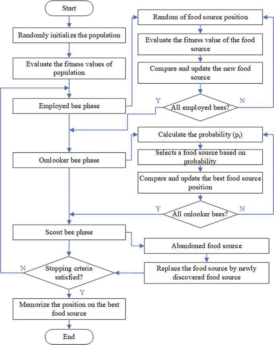
Flowchart of Artificial Bee Colony (ABC) algorithm
ABC algorithm was used in many fields such as job shop scheduling [6,7], binary optimization [8–10], travelling salesman [11], digital signal processing [63], and so on. For example, Mizan et al. [18] presented job scheduling in Hybrid cloud by modifying Bee Life algorithm and Greedy algorithm to achieve an affirmative response from the end users and utilize the resources. Accordingly, the objective of this study is to optimize task scheduling, resource allocation, and load balancing using applying Heuristic Task Scheduling with Artificial Bee Colony (HABC) based on the proposed reducing or minimizing makespan in cloud computing environment. This research focused on both cases of homogeneous and heterogeneous environments and investigated how efficient the HABC algorithm performed when the tasks in the system were increased and the data distribution was changed.
3. LOAD BALANCING ALGORITHM INSPIRED BY ARTIFICIAL BEE COLONY AND HEURISTIC SCHEDULING ALGORITHM
Cloud computing utilizes different resources depending on the types of user's request. Moreover, fulfilment of the request of service depends on workload of servers. If a cloud system has an efficient task scheduling, it will help reduce the makespan and balance the workload among the servers. In Ref. [19] and Ref. [20], ABC algorithm was used to manage VMs scheduling in cloud computing within a homogeneous environment. However, since the specifications of current servers are very different, ABC algorithm with heuristic task scheduling was also applied to a heterogeneous environment in this study. The two goals of the proposed method were to obtain a good workload balance for maximum productivity and minimize total makespan. This section describes the heuristic scheduling algorithm and the proposed scheduling algorithm.
3.1. Heuristic Scheduling Algorithm
Heuristic method is an approach to problem solving using rules such as priority rule or using a random method to find an optimal solution for a problem. A heuristic method may provide a good result, but it cannot guarantee an optimal solution. Nevertheless, it is simple to use. A heuristic task scheduling with priority as a criterion for selecting a process in a system was used in this study because it is a basic method for scheduling tasks [64,65]. We selected the following 3 simple priority criteria for investigation [66]:
First Come First Serve (FCFS): is a task scheduling scheme that processes the first job that the user has requested first.
Smallest Job First (SJF): is a task scheduling scheme that processes with the smallest job first
Largest Job First (LJF): is a task scheduling scheme that processes the largest job first.
3.2. Proposed Method
Let
First step: the number of bees (n) in the population was specified. They were assigned randomly to go to all of the different food sources (m) that represented the VMs and their fitness values were calculated, therefore initializing the VMs as shown in Algorithm 1.
Algorithm 1: Initialization
1. For i = 1 to n
2. Send the population of bees into the system to find appropriate VMs by Random search.
3. Calculate the fitness of each VM by using (1)
where j = index of the VM that the ith bee found.4. End For
-
Second step: a different default value was assigned to each food source according to the specifications of the VM. Bees were grouped into 3 types: Scout Bees, Employed Bees, and Onlooker Bees. A Scout Bee found the initial position of a food source. An Employed Bee went to the food source, recalculated and updated the fitness value of food source. An Onlooker Bee decided which food source was the best food source. The operation of an employed bee is presented in Algorithm 2.
Algorithm 2: Employed bee phase
1. For i = 1 to n
2. Employed bees are sent randomly to food sources (VMs in cloud computing).
3. Fitness of each VM is calculated based on (2)
4. Update the fitness value
5. End For
-
Third step: the Employed bees have searched around for food sources, they brought back information about the food sources to the Onlooker bee. The Onlooker bee then recalculated the fitness values of the food sources. The operation of the onlooker bee is shown in Algorithm 3.
Algorithm 3: Onlooker bee phase
1. The onlooker bee chooses the first m food sources (VM) with the highest fitness values and perform “Neighborhood Search” around the food sources
2. An nsp number of employed bees are sent to bring back new positions of the first m food sources while a nep number of employed bees are sent to all food sources to bring back new positions of these food sources; all of them come back to relay the information to the onlooker bee
3. The onlooker bee calculates the new fitness values of the food sources according to (3),
where4. The onlooker bee chooses the best food source (VM) and assigns a task to the VM
-
Fourth step: the employed bee that was the owner of the best food source was then transformed into a scout bee. The operation of a scout bee is shown in Algorithm 4.
Algorithm 4: Scout bee phase
1. If food source = null then
2. Send the previously transformed scout bee into the system to find an appropriate VM by Random search.
3. Calculate the fitness value of that VM by using (1)
4. End If
-
Fifth step: the overall operation of HABC algorithm is described in Algorithm 5.
Algorithm 5: Improved HABC Algorithm
Input: Dataset, Bee's Parameters;
Output: Minimum makespan;
1. Initialize the individual in the population.
2. Set the default values of the food sources (VM) by using (2).
3. Initialization (Algorithm 1)
4. Repeat
5. Employed bee phase(Algorithm 2)
6. Onlooker bee phase (Algorithm 3)
7. Calculate the load balance value of the system after task scheduling on VMs. It is calculated by using Standard Deviation (S.D.) [67] as in (4) and (5),
The processing time for each VM (Xj) is calculated according to (6),
The average processing time for running a VM in the system (
If
8. Scout bee phase (Algorithm 4)
9. Until (the termination condition is met)
| Symbol | Definition |
|---|---|
| m | The number of virtual machines (VMs) |
| The set of VM | |
| K | The total number of tasks the system has to perform |
| The set of tasks | |
| N | The total number of bees performing in the algorithmic procedure |
| Cj | The performance of the jth virtual machine |
| Pe | The number of processors in the VM |
| Mi | Million Instructions Per Second (MIPS) |
| Bw | Bandwidth of VM |
| F | Fitness |
| Tl | The length of task in MIa |
| Pi | Probability that the ith food source is good which depends on its fitness value, |
Variables used in this study and their definitions.
4. EXPERIMENTAL RESULTS
4.1. System Environment Parameter Settings
The algorithms: HABC, ACO, PSO, and IPSO described were run using CloudSim-3.0.1 [68,69] tools on a personal computer. The experiments were performed on 10 data centers and 50 VMs. In the experiments, we focused on both kinds of environments: homogeneous and heterogeneous environments in cloud computing.
For each VM in cloud computing within a homogeneous environment, the following parameters were set: Instructions Per Second in millions (MIPS is a measurement of the processing speed of a computer) of Processing Element (PE) were fixed at 9726; Number of PE per VM was fixed at 1; and RAM used was fixed at 1024 Megabytes (MB).
For each VM in cloud computing within a heterogeneous environment, the following parameters were set: MIPS were in the range of 5000–9726; Number of PE per VM was fixed at 2; RAM used was set in the range of 512–4096 MB; and Bandwidth was set in the range of 1000–10000.
4.2. The Datasets Used in the Experiments
To evaluate the effectiveness of the proposed approach, twelve datasets, shown in Table 2, were used. Those datasets were of 4 types. The set D1–D3 of the first type was a set of random information, i.e., there are no definite terms, no specific format, and no specific distribution of information. The set D4–D6 of the second type was a set of random data with normal distribution. The set D7–D9 of the third type was a set of random data with a Right-Skewed Distribution [70]. Lastly, the set D10–D12 of the fourth type was a set of random data with a Left-Skewed Distribution. Each type of datasets had a different range of job size and each dataset comprised a number of groups of 100, 200, 300, …, 1500 submitted tasks.
| Type of Dataset | Dataset Name | Length of Task (MIa) |
|---|---|---|
| Random | D1 | [5000, 20000] |
| D2 | [15000, 35000] | |
| D3 | [25000, 45000] | |
| Normal distribution | D4 | [5000, 20000] |
| D5 | [15000, 35000] | |
| D6 | [25000, 45000] | |
| Right-skewed distributionb | D7 | [5000, 20000] |
| D8 | [15000, 35000] | |
| D9 | [25000, 45000] | |
| Left-skewed distributionc | D10 | [5000, 20000] |
| D11 | [15000, 35000] | |
| D12 | [25000, 45000] |
MI is Million Instruction.
Positively Skewed Curve.
Negatively Skewed Curve.
The datasets used in the experiments.
4.3. Parameters Settings for the Proposed Algorithm and the Comparing Algorithms
In these experiments, we have determined the parameters of the population and various conditions according to the related works, which are referred to HABC [20], ACO [55,56], PSO [48], and IPSO [49]. It is well known that these parameters are highly effect on the algorithms. The determination of parameters is varied according to the dimension of problems or characteristics. One reason that we need tuning the parameters [20] is in order to get the suitable parameters for the pattern of problems and datasets. However, we do not claim that the proposed algorithm or the specified parameters outperform other algorithms for all types of problems and datasets. Therefore, tuning parameters is the best way to get the suitable parameters to solve problems.
The experiments had been performed to determine the optimal bee parameters for the proposed algorithm [20] which are shown in Table 3. In addition, the scheduling performance of the proposed algorithm was also compared with those of ACO [55,56], PSO [48], and IPSO [49] that used the parameter settings as shown in Table 3.
| HABC [20] |
ACO [55,56] |
PSO [48] |
IPSO [49] |
||||
|---|---|---|---|---|---|---|---|
| Parameter | Values | Parameter | Values | Parameter | Values | Parameter | Values |
| Number of scout bees (n) | 960 | Ants | 50 | Number of particles | 100 | Population size | 100 |
| Number of sites selected out of n visited sites (m) | 96 | Maximum probability of trial | 0.98 | Weight (w) | 0.9 | Weight (wmin, wmax) | 0.1, 0.9 |
| Number of best sites out of m selected sites (e) | 1 | Local search probability | 0.01 | Acceleration factor (C1) | 1.49445 | Acceleration factor (C1) | 1.49445 |
| Number of bees recruited for searching best e sites (nep) | 768 | Evaporation rate | 0.01 | Acceleration factor (C2) | 1.49445 | Acceleration factor (C2) | 1.49445 |
| Number of bees recruited for searching other (m-e) selected sites (nsp) | 192 | Max number of iterations | 1000 | Max number of iterations | 1000 | Maximum iterations | 1000 |
| Max number of iterations | 1000 | K | 5 | ||||
HABC, Heuristic Task Scheduling with Artificial Bee Colony; ACO, Ant Colony Optimization; PSO, Particle Swarm Optimization; IPSO, improved PSO.
The values of the parameters used in the proposed algorithm and in the other comparison algorithms.
Those optimal settings were based on the original papers. The number of iterations that each algorithm would be run in the experiment was 20.
4.4. Experimental Results and Discussions
In one of our previous papers [20], the performances of the proposed algorithm in combination with 3 heuristics-HABC_FCFS, HABC_LJF, and HABC_SJF-were compared with those of the heuristics alone-FCFS, LJF, and SJF. The results of previous experiments showed that when the largest job was considered first (HABC_LJF), its scheduling performance was better than those of HABC_FCFS and HABC_SJF.
The HABC_LJF also balanced the load of submitted tasks with minimal makespan. In this paper, we used 2 VM environments: heterogeneous and homogeneous to evaluate the performance of HABC_LJF method on different datasets and to compare it with other scheduling algorithms. The number of VMs was fixed throughout the experiment but the number of tasks was increased in 100 incremental steps from 100 to 1,500 tasks.
In the evaluation of the performance of HABC_LJF algorithm in cloud computing, we divided our experiment into two parts. In the first part, the datasets of various types as described in Table 3 were used. In the second part, the performance of the heuristic task scheduling with ABC in terms of load imbalance was evaluated. In the first part, the performance evaluation was performed on 4 cases according to the type of datasets used. The following are the results of the 4 cases for evaluation of the makespan.
Case 1: Random datasets
The makespan of HABC_LJF running on random datasets D1–D3 was compared with those of ACO, PSO, and IPSO algorithms. The number of groups of submitted tasks was varied in each run from 100 to 1500 submitted tasks in an increment of 100 tasks. The average makespan for 300, 900, and 1,500 tasks in cloud computing within homogeneous and heterogeneous environments are shown in Tables 4 and 5, respectively. Actually, a higher number of tasks were run but the results are not shown here due to lack of space.
| Dataset | Task | Variable | HABC_LJF | ACO_FCFS | ACO_LJF | ACO_SJF | PSO_FCFS | PSO_LJF | PSO_SJF | IPSO_FCFS | IPSO_LJF | IPSO_SJF |
|---|---|---|---|---|---|---|---|---|---|---|---|---|
| D1 | 300 | Min | 8.623 | 9.600 | 9.023 | 9.982 | 25.982 | 25.030 | 25.707 | 29.578 | 27.448 | 27.979 |
| Max | 8.643 | 10.592 | 9.343 | 11.017 | 29.017 | 26.329 | 26.408 | 32.381 | 31.162 | 34.342 | ||
| Avg | 8.633 | 10.227 | 9.225 | 10.324 | 26.988 | 25.563 | 25.876 | 30.626 | 28.766 | 30.273 | ||
| 900 | Min | 25.015 | 26.352 | 25.739 | 26.702 | 83.733 | 81.206 | 83.467 | 107.237 | 103.885 | 105.384 | |
| Max | 25.262 | 27.369 | 26.042 | 27.561 | 84.777 | 96.767 | 86.560 | 113.512 | 108.464 | 107.781 | ||
| Avg | 25.073 | 26.819 | 25.881 | 26.976 | 84.165 | 89.705 | 84.255 | 109.620 | 105.725 | 106.302 | ||
| 1500 | Min | 42.275 | 43.641 | 42.892 | 44.050 | 151.965 | 153.637 | 153.482 | 215.075 | 211.427 | 303.934 | |
| Max | 42.614 | 45.020 | 43.523 | 45.058 | 164.660 | 156.171 | 157.010 | 229.624 | 315.327 | 319.373 | ||
| Avg | 42.409 | 44.233 | 43.228 | 44.641 | 158.947 | 154.736 | 154.529 | 222.093 | 262.953 | 310.891 | ||
| D2 | 300 | Min | 16.308 | 18.685 | 18.036 | 19.148 | 36.465 | 32.567 | 33.462 | 37.476 | 35.041 | 37.075 |
| Max | 16.341 | 19.719 | 18.288 | 20.252 | 39.547 | 34.134 | 35.205 | 39.296 | 42.372 | 39.112 | ||
| Avg | 16.319 | 19.258 | 18.161 | 19.646 | 38.194 | 32.993 | 33.906 | 38.645 | 38.841 | 37.428 | ||
| 900 | Min | 48.340 | 50.969 | 50.150 | 51.526 | 108.373 | 105.943 | 106.805 | 129.830 | 128.848 | 127.957 | |
| Max | 48.907 | 52.823 | 51.427 | 53.980 | 109.092 | 108.074 | 108.557 | 137.917 | 132.341 | 130.492 | ||
| Avg | 48.475 | 51.795 | 50.353 | 52.154 | 108.704 | 106.622 | 107.725 | 133.191 | 130.587 | 129.206 | ||
| 1500 | Min | 80.237 | 82.888 | 81.959 | 83.918 | 192.893 | 189.624 | 194.519 | 250.603 | 245.937 | 248.938 | |
| Max | 81.623 | 84.951 | 83.743 | 86.442 | 193.491 | 192.754 | 198.249 | 263.329 | 256.496 | 254.803 | ||
| Avg | 80.516 | 84.122 | 82.818 | 85.263 | 193.206 | 191.226 | 196.048 | 255.369 | 251.500 | 251.033 | ||
| D3 | 300 | Min | 22.229 | 25.645 | 24.983 | 26.244 | 40.877 | 38.553 | 39.606 | 45.246 | 45.293 | 46.121 |
| Max | 22.262 | 27.500 | 25.278 | 26.867 | 42.182 | 41.206 | 41.803 | 56.463 | 50.604 | 50.163 | ||
| Avg | 22.244 | 26.378 | 25.126 | 26.529 | 41.230 | 39.237 | 40.155 | 49.921 | 47.083 | 47.706 | ||
| 900 | Min | 67.077 | 70.642 | 70.006 | 71.203 | 127.109 | 125.271 | 125.686 | 158.775 | 158.025 | 160.241 | |
| Max | 67.245 | 73.066 | 72.770 | 74.383 | 128.451 | 128.572 | 128.420 | 176.779 | 174.420 | 169.610 | ||
| Avg | 67.188 | 71.676 | 70.506 | 72.115 | 127.780 | 126.110 | 126.468 | 169.075 | 165.177 | 164.849 | ||
| 1500 | Min | 111.770 | 116.333 | 114.901 | 116.010 | 223.859 | 222.317 | 223.264 | 290.299 | 290.595 | 290.642 | |
| Max | 112.050 | 119.118 | 118.887 | 119.478 | 227.468 | 225.851 | 225.024 | 304.952 | 289.595 | 300.847 | ||
| Avg | 111.870 | 117.533 | 116.918 | 118.256 | 225.457 | 223.576 | 224.219 | 296.090 | 293.595 | 294.004 |
HABC, Heuristic Task Scheduling with Artificial Bee Colony; ACO, Ant Colony Optimization; PSO, Particle Swarm Optimization; IPSO, improved PSO; FCFS, First Come First Serve; SJF, Smallest Job First; LJF, Largest Job First.
The comparison of the average makespan of the systems with HABC, ACO, PSO, and IPSO in a homogeneous environment with datasets D1 – D3.
| Dataset | Task | Variable | HABC_LJF | ACO_FCFS | ACO_LJF | ACO_SJF | PSO_FCFS | PSO_LJF | PSO_SJF | IPSO_FCFS | IPSO_LJF | IPSO_SJF |
|---|---|---|---|---|---|---|---|---|---|---|---|---|
| D1 | 300 | Min | 7.320 | 7.982 | 7.500 | 8.292 | 24.207 | 23.707 | 25.749 | 27.498 | 26.623 | 27.055 |
| Max | 7.368 | 9.803 | 8.181 | 9.925 | 27.171 | 24.370 | 26.155 | 30.966 | 29.537 | 27.616 | ||
| Avg | 7.345 | 8.817 | 7.765 | 9.086 | 25.610 | 23.996 | 26.007 | 28.792 | 27.144 | 27.322 | ||
| 900 | Min | 20.601 | 21.133 | 20.605 | 21.707 | 80.445 | 79.467 | 81.114 | 101.135 | 98.005 | 99.690 | |
| Max | 20.865 | 23.311 | 21.808 | 22.592 | 82.856 | 81.043 | 88.297 | 106.207 | 111.467 | 101.623 | ||
| Avg | 20.715 | 22.256 | 20.941 | 22.146 | 81.698 | 79.943 | 82.409 | 102.858 | 100.261 | 100.695 | ||
| 1500 | Min | 34.213 | 34.976 | 34.218 | 35.310 | 148.688 | 148.288 | 148.757 | 216.645 | 213.903 | 219.464 | |
| Max | 34.717 | 37.461 | 35.203 | 35.970 | 152.961 | 150.648 | 151.124 | 247.682 | 256.862 | 247.018 | ||
| Avg | 34.450 | 36.114 | 34.700 | 35.630 | 150.867 | 149.111 | 149.999 | 227.404 | 232.807 | 231.975 | ||
| D2 | 300 | Min | 14.595 | 15.385 | 14.935 | 15.933 | 32.330 | 30.390 | 33.420 | 32.324 | 32.507 | 34.153 |
| Max | 14.687 | 18.406 | 15.641 | 17.333 | 36.045 | 30.760 | 33.823 | 34.935 | 34.675 | 35.080 | ||
| Avg | 14.615 | 16.978 | 15.316 | 16.839 | 33.353 | 30.545 | 33.666 | 33.442 | 33.155 | 34.533 | ||
| 900 | Min | 40.299 | 40.305 | 40.486 | 41.219 | 98.444 | 96.444 | 98.889 | 118.667 | 118.246 | 119.673 | |
| Max | 40.706 | 44.432 | 41.102 | 43.978 | 101.081 | 97.356 | 100.745 | 131.408 | 123.997 | 124.640 | ||
| Avg | 40.439 | 42.816 | 40.821 | 42.402 | 99.779 | 96.823 | 99.582 | 124.194 | 119.795 | 121.197 | ||
| 1500 | Min | 65.784 | 66.160 | 66.063 | 66.240 | 175.483 | 175.397 | 169.006 | 229.331 | 230.574 | 233.232 | |
| Max | 67.162 | 69.771 | 67.677 | 68.459 | 181.691 | 178.763 | 204.867 | 261.110 | 261.855 | 237.858 | ||
| Avg | 66.243 | 67.947 | 66.418 | 67.835 | 177.890 | 177.211 | 180.840 | 239.835 | 237.419 | 234.780 | ||
| D3 | 300 | Min | 20.374 | 21.310 | 20.541 | 22.037 | 36.164 | 35.042 | 38.526 | 38.310 | 36.574 | 40.152 |
| Max | 20.595 | 25.453 | 21.479 | 23.777 | 41.005 | 35.376 | 39.248 | 42.268 | 39.352 | 40.698 | ||
| Avg | 20.412 | 23.130 | 21.084 | 22.705 | 38.605 | 35.183 | 38.678 | 39.821 | 38.069 | 40.422 | ||
| 900 | Min | 56.053 | 56.317 | 56.796 | 57.418 | 114.889 | 108.005 | 109.332 | 128.071 | 125.720 | 129.099 | |
| Max | 56.986 | 61.682 | 57.280 | 59.408 | 118.975 | 109.462 | 112.828 | 135.651 | 129.380 | 131.149 | ||
| Avg | 56.632 | 58.188 | 57.014 | 58.687 | 116.954 | 108.515 | 110.325 | 130.650 | 127.624 | 130.120 | ||
| 1500 | Min | 92.419 | 93.852 | 93.374 | 93.751 | 195.333 | 196.762 | 191.022 | 264.640 | 244.018 | 245.887 | |
| Max | 92.945 | 96.593 | 93.358 | 94.951 | 222.115 | 219.735 | 195.878 | 316.860 | 278.675 | 251.534 | ||
| Avg | 92.624 | 95.327 | 93.005 | 94.492 | 205.862 | 207.061 | 192.619 | 285.370 | 256.390 | 248.354 |
HABC, Heuristic Task Scheduling with Artificial Bee Colony; ACO, Ant Colony Optimization; PSO, Particle Swarm Optimization; IPSO, improved PSO; FCFS, First Come First Serve; SJF, Smallest Job First; LJF, Largest Job First.
The comparison of the average makespan of the systems with HABC, ACO, PSO, and IPSO in a heterogeneous environment with datasets D1 – D3.
According to Table 4, HABC_LJF performed the best as the number of tasks was increased. Moreover, the minimum makespan, the maximum makespan, and the average makespan, all three of them were the lowest. The performance of HABC_LJF was outstanding in the homogeneous environment.
In addition, in order to observe the effect of the range of job size on performance scalability of the system, we evaluated the average makespan with three datasets that had different ranges of job size (D1–D3). The results show that the HABC_LJF algorithm also outperformed the others for all size ranges tested in the homogeneous environment.
The results for the average makespan of HABC_LJF algorithm and the other algorithms with an increasing number of submitted tasks in cloud computing within a heterogeneous environment when used with random datasets are shown in Table 5. The performance of HABC_LJF was the best because its minimum makespan, maximum makespan, and average makespan were mostly the lowest in cloud computing within a heterogeneous environment. Furthermore, when datasets with different ranges of job size were used, HABC_LJF still outperformed the others in the same way that it did in homogeneous environment.
Case 2: Random data with a normal distribution
Table 6 shows the makespan of every algorithm tested with datasets (D4–D6) : random datasets with normal distribution. The results showed that the HABC_LJF used the lowest minimum makespan, the lowest maximum makespan, and the lowest average makespan than the other algorithms did in the homogeneous environment.
| Dataset | Task | Variable | HABC_LJF | ACO_FCFS | ACO_LJF | ACO_SJF | PSO_FCFS | PSO_LJF | PSO_SJF | IPSO_FCFS | IPSO_LJF | IPSO_SJF |
|---|---|---|---|---|---|---|---|---|---|---|---|---|
| D4 | 300 | Min | 8.575 | 9.883 | 9.111 | 10.170 | 25.540 | 24.501 | 25.472 | 29.994 | 28.758 | 28.635 |
| Max | 8.634 | 11.052 | 9.501 | 10.740 | 26.333 | 24.940 | 26.308 | 32.600 | 31.167 | 29.165 | ||
| Avg | 8.584 | 10.331 | 9.308 | 10.434 | 25.798 | 24.643 | 25.813 | 30.624 | 29.298 | 28.851 | ||
| 900 | Min | 25.582 | 27.020 | 26.319 | 27.101 | 82.715 | 81.997 | 84.421 | 110.198 | 107.394 | 107.813 | |
| Max | 25.867 | 27.866 | 26.746 | 28.302 | 92.448 | 84.768 | 87.776 | 119.204 | 110.113 | 110.444 | ||
| Avg | 25.669 | 27.400 | 26.511 | 27.644 | 84.544 | 83.432 | 85.733 | 113.127 | 108.915 | 109.174 | ||
| 1500 | Min | 41.993 | 43.462 | 42.731 | 43.983 | 149.972 | 152.230 | 151.124 | 221.121 | 215.575 | 218.054 | |
| Max | 42.246 | 44.370 | 44.234 | 44.703 | 157.576 | 154.169 | 161.643 | 233.171 | 220.500 | 221.989 | ||
| Avg | 42.140 | 43.799 | 43.177 | 44.364 | 152.614 | 153.111 | 153.875 | 225.417 | 217.941 | 219.824 | ||
| D5 | 300 | Min | 16.182 | 18.335 | 17.793 | 18.982 | 34.274 | 32.607 | 33.625 | 37.653 | 38.349 | 37.446 |
| Max | 16.215 | 20.528 | 19.076 | 20.624 | 35.227 | 34.275 | 34.922 | 42.583 | 40.628 | 37.899 | ||
| Avg | 16.194 | 19.098 | 18.004 | 19.429 | 34.484 | 32.893 | 33.952 | 40.022 | 38.938 | 37.747 | ||
| 900 | Min | 48.367 | 51.071 | 50.232 | 51.457 | 108.799 | 106.392 | 107.270 | 135.063 | 129.111 | 130.951 | |
| Max | 48.499 | 52.978 | 51.790 | 54.115 | 118.703 | 108.260 | 108.692 | 138.506 | 134.602 | 134.658 | ||
| Avg | 48.404 | 52.034 | 50.572 | 52.473 | 110.707 | 107.140 | 107.825 | 136.418 | 132.357 | 132.098 | ||
| 1500 | Min | 80.594 | 83.666 | 82.612 | 83.878 | 193.607 | 192.516 | 192.841 | 258.106 | 252.917 | 254.743 | |
| Max | 80.808 | 85.558 | 84.510 | 86.401 | 256.281 | 194.782 | 194.970 | 285.920 | 270.308 | 258.800 | ||
| Avg | 80.701 | 84.506 | 83.578 | 85.431 | 207.942 | 193.393 | 193.883 | 263.625 | 258.098 | 256.448 | ||
| D6 | 300 | Min | 22.266 | 25.403 | 24.843 | 26.012 | 40.675 | 38.361 | 39.239 | 45.958 | 45.530 | 44.446 |
| Max | 22.322 | 27.499 | 25.273 | 27.442 | 40.989 | 43.362 | 46.370 | 47.159 | 49.020 | 45.375 | ||
| Avg | 22.275 | 26.316 | 25.094 | 26.585 | 40.832 | 39.170 | 41.054 | 46.464 | 46.335 | 44.698 | ||
| 900 | Min | 66.586 | 70.473 | 69.570 | 70.620 | 125.921 | 123.478 | 123.851 | 151.630 | 150.560 | 149.820 | |
| Max | 66.733 | 72.472 | 71.977 | 73.627 | 126.799 | 126.650 | 127.080 | 157.917 | 157.273 | 151.973 | ||
| Avg | 66.675 | 71.373 | 70.054 | 71.545 | 126.492 | 124.704 | 125.075 | 154.434 | 152.390 | 151.096 | ||
| 1500 | Min | 111.167 | 115.941 | 114.366 | 115.366 | 223.019 | 221.505 | 222.173 | 287.264 | 281.794 | 285.184 | |
| Max | 111.508 | 117.362 | 117.450 | 118.750 | 226.545 | 259.360 | 224.472 | 297.683 | 292.236 | 293.692 | ||
| Avg | 111.291 | 116.548 | 116.070 | 117.391 | 224.414 | 238.211 | 223.379 | 291.949 | 288.023 | 287.741 |
HABC, Heuristic Task Scheduling with Artificial Bee Colony; ACO, Ant Colony Optimization; PSO, Particle Swarm Optimization; IPSO, improved PSO; FCFS, First Come First Serve; SJF, Smallest Job First; LJF, Largest Job First.
The comparison of the average makespan of the systems with HABC, ACO, PSO, and IPSO in a homogeneous environment with datasets D4 – D6.
The makespan of the algorithms working within a heterogeneous environment when random datasets with normal distribution were used are shown in Table 7. The results show that for the datasets that had different ranges of job size, HABC_LJF outperformed the others in the same way as they did in a homogeneous environment except for the case of dataset D4 and D6. For the case of dataset D4with the number of submitted tasks equaled to 900, the ACO_LJF gave the lowest minimum makespan. Meanwhile, the D6 dataset with 900 submitted tasks in which ACO_LJF used the lowest minimum makespan and ACO_SJF used the lowest maximum makespan. However, this makespan was not very different from that used by HABC_LJF. When the makespan for all cases were considered, HABC_LJF still outperformed the other algorithms.
| Dataset | Task | Variable | HABC_LJF | ACO_FCFS | ACO_LJF | ACO_SJF | PSO_FCFS | PSO_LJF | PSO_SJF | IPSO_FCFS | IPSO_LJF | IPSO_SJF |
|---|---|---|---|---|---|---|---|---|---|---|---|---|
| D4 | 300 | Min | 7.347 | 8.266 | 7.460 | 8.378 | 25.131 | 23.905 | 24.550 | 28.075 | 28.058 | 28.192 |
| Max | 7.536 | 9.874 | 7.993 | 9.678 | 27.318 | 25.652 | 25.811 | 33.277 | 29.661 | 30.436 | ||
| Avg | 7.429 | 9.157 | 7.711 | 9.006 | 25.850 | 24.791 | 24.849 | 30.191 | 28.811 | 28.953 | ||
| 900 | Min | 20.822 | 21.427 | 20.973 | 22.206 | 79.248 | 81.988 | 77.327 | 98.817 | 96.358 | 98.507 | |
| Max | 21.869 | 23.342 | 21.397 | 23.313 | 81.374 | 85.940 | 78.608 | 103.967 | 98.902 | 101.255 | ||
| Avg | 21.215 | 22.360 | 21.226 | 22.597 | 80.299 | 84.128 | 77.870 | 100.968 | 97.827 | 99.515 | ||
| 1500 | Min | 33.862 | 34.144 | 33.987 | 34.943 | 141.381 | 140.255 | 140.594 | 199.534 | 195.573 | 197.259 | |
| Max | 34.482 | 36.491 | 35.618 | 35.978 | 162.631 | 153.213 | 144.570 | 211.162 | 201.047 | 202.690 | ||
| Avg | 34.210 | 35.305 | 34.399 | 35.434 | 151.768 | 144.389 | 142.179 | 203.859 | 198.525 | 199.162 | ||
| D5 | 300 | Min | 14.211 | 14.876 | 14.837 | 16.105 | 25.131 | 23.905 | 24.550 | 33.591 | 32.701 | 34.567 |
| Max | 14.306 | 18.346 | 15.362 | 17.862 | 27.318 | 25.652 | 25.811 | 37.458 | 33.676 | 35.061 | ||
| Avg | 14.261 | 16.768 | 15.100 | 16.640 | 25.850 | 24.791 | 24.849 | 35.377 | 33.052 | 34.751 | ||
| 900 | Min | 40.087 | 41.393 | 40.543 | 41.148 | 79.248 | 81.988 | 77.327 | 116.100 | 114.003 | 117.011 | |
| Max | 40.735 | 47.170 | 41.090 | 42.831 | 81.374 | 85.940 | 78.608 | 122.000 | 116.834 | 118.787 | ||
| Avg | 40.256 | 43.287 | 40.754 | 42.407 | 80.299 | 84.128 | 77.870 | 118.567 | 115.730 | 117.796 | ||
| 1500 | Min | 66.087 | 66.979 | 66.228 | 66.660 | 141.381 | 140.255 | 140.594 | 231.830 | 228.575 | 230.755 | |
| Max | 66.948 | 70.342 | 67.070 | 72.701 | 162.631 | 153.213 | 144.570 | 242.655 | 233.695 | 235.654 | ||
| Avg | 66.407 | 68.998 | 66.679 | 68.511 | 151.768 | 144.389 | 142.179 | 236.277 | 231.274 | 233.031 | ||
| D6 | 300 | Min | 20.300 | 21.324 | 20.600 | 21.816 | 35.892 | 34.222 | 38.002 | 38.696 | 37.067 | 40.703 |
| Max | 20.606 | 25.610 | 21.514 | 23.305 | 39.573 | 34.525 | 38.280 | 43.352 | 38.837 | 41.195 | ||
| Avg | 20.412 | 23.303 | 21.077 | 22.851 | 37.991 | 34.350 | 38.112 | 40.338 | 38.347 | 40.964 | ||
| 900 | Min | 55.891 | 55.881 | 56.112 | 57.728 | 107.681 | 104.625 | 108.412 | 129.248 | 127.836 | 130.677 | |
| Max | 56.877 | 60.508 | 56.811 | 59.122 | 109.710 | 106.115 | 110.034 | 135.833 | 131.669 | 132.884 | ||
| Avg | 56.185 | 58.464 | 56.507 | 58.322 | 108.418 | 105.422 | 108.966 | 131.469 | 129.420 | 131.899 | ||
| 1500 | Min | 92.022 | 93.339 | 92.170 | 93.697 | 188.914 | 188.526 | 190.508 | 251.495 | 249.411 | 250.938 | |
| Max | 93.022 | 98.200 | 93.025 | 94.655 | 194.341 | 191.091 | 192.220 | 264.148 | 253.773 | 256.640 | ||
| Avg | 92.032 | 95.466 | 92.498 | 94.106 | 191.243 | 189.838 | 191.406 | 255.573 | 251.396 | 253.024 |
HABC, Heuristic Task Scheduling with Artificial Bee Colony; ACO, Ant Colony Optimization; PSO, Particle Swarm Optimization; IPSO, improved PSO; FCFS, First Come First Serve; SJF, Smallest Job First; LJF, Largest Job First.
The comparison of the average makespan of the systems with HABC, ACO, PSO, and IPSO in a heterogeneous environment with datasets D4 – D6.
Case 3: Random data with Right-Skewed Distribution
Tables 8 and 9 show the results obtained from using datasets (D7–D9)—random datasets with Right-Skewed Distribution—in homogeneous and heterogeneous environments, respectively. The experimental results indicate that HABC_LJF used the lowest minimum makespan, the lowest maximum makespan, and the lowest average makespan than the other algorithms did in the homogeneous environment. The results were the same as in Case 1.
| Dataset | Task | Variable | HABC_LJF | ACO_FCFS | ACO_LJF | ACO_SJF | PSO_FCFS | PSO_LJF | PSO_SJF | IPSO_FCFS | IPSO_LJF | IPSO_SJF |
|---|---|---|---|---|---|---|---|---|---|---|---|---|
| D7 | 300 | Min | 8.173 | 9.523 | 8.788 | 9.600 | 25.399 | 24.606 | 25.048 | 28.675 | 28.359 | 28.078 |
| Max | 8.248 | 10.350 | 9.068 | 10.213 | 25.589 | 24.846 | 26.086 | 29.708 | 30.863 | 28.928 | ||
| Avg | 8.211 | 9.951 | 8.950 | 9.904 | 25.524 | 24.696 | 25.554 | 29.090 | 29.149 | 28.515 | ||
| 900 | Min | 23.742 | 25.072 | 24.179 | 25.155 | 83.196 | 81.680 | 81.820 | 106.287 | 104.397 | 105.338 | |
| Max | 24.130 | 26.153 | 24.727 | 26.494 | 83.696 | 82.620 | 83.303 | 110.536 | 106.107 | 109.230 | ||
| Avg | 23.874 | 25.520 | 24.384 | 25.640 | 83.526 | 82.159 | 82.205 | 107.879 | 105.350 | 106.786 | ||
| 1500 | Min | 39.575 | 41.225 | 40.088 | 41.291 | 151.844 | 149.901 | 150.912 | 227.688 | 211.238 | 214.100 | |
| Max | 39.866 | 42.121 | 40.807 | 42.272 | 152.875 | 152.081 | 152.960 | 239.956 | 228.046 | 230.281 | ||
| Avg | 39.679 | 41.569 | 40.433 | 41.866 | 152.226 | 151.149 | 152.024 | 232.735 | 216.979 | 224.078 | ||
| D8 | 300 | Min | 14.604 | 16.839 | 16.258 | 17.553 | 32.596 | 32.379 | 23.083 | 37.881 | 37.521 | 36.366 |
| Max | 14.622 | 19.080 | 16.541 | 18.576 | 33.470 | 34.339 | 23.167 | 39.898 | 38.762 | 37.016 | ||
| Avg | 14.613 | 17.792 | 16.406 | 17.829 | 32.839 | 33.012 | 23.097 | 38.637 | 37.980 | 36.641 | ||
| 900 | Min | 44.195 | 46.969 | 45.842 | 47.344 | 107.407 | 106.832 | 67.939 | 132.910 | 131.491 | 130.931 | |
| Max | 44.310 | 48.608 | 47.310 | 49.409 | 121.232 | 107.571 | 68.224 | 139.303 | 135.710 | 132.904 | ||
| Avg | 44.234 | 47.815 | 46.140 | 48.094 | 115.012 | 107.174 | 68.018 | 135.926 | 133.278 | 131.848 | ||
| 1500 | Min | 73.733 | 77.107 | 75.205 | 76.916 | 193.523 | 189.848 | 113.247 | 248.315 | 245.764 | 248.212 | |
| Max | 75.611 | 78.529 | 77.193 | 78.873 | 201.949 | 192.243 | 113.367 | 260.620 | 252.230 | 253.200 | ||
| Avg | 74.095 | 77.772 | 76.394 | 78.122 | 197.262 | 191.025 | 113.305 | 253.714 | 249.900 | 250.838 | ||
| D9 | 300 | Min | 20.098 | 23.697 | 22.668 | 23.842 | 38.213 | 36.604 | 37.460 | 43.877 | 43.646 | 42.599 |
| Max | 20.174 | 24.954 | 23.046 | 24.824 | 38.548 | 36.794 | 37.628 | 45.133 | 47.313 | 43.088 | ||
| Avg | 20.126 | 24.223 | 22.818 | 24.297 | 38.421 | 36.713 | 37.548 | 44.439 | 44.296 | 42.790 | ||
| 900 | Min | 60.023 | 63.854 | 62.451 | 64.003 | 120.953 | 118.471 | 89.919 | 145.600 | 146.591 | 141.441 | |
| Max | 60.302 | 66.557 | 64.231 | 67.714 | 121.867 | 119.243 | 97.388 | 149.600 | 170.342 | 161.315 | ||
| Avg | 60.181 | 64.803 | 62.795 | 64.750 | 121.292 | 118.856 | 92.890 | 146.600 | 152.863 | 150.354 | ||
| 1500 | Min | 99.961 | 104.231 | 102.648 | 104.687 | 214.429 | 213.021 | 177.504 | 278.953 | 268.821 | 267.217 | |
| Max | 100.364 | 106.827 | 105.310 | 107.602 | 217.676 | 244.700 | 203.813 | 309.324 | 323.782 | 283.917 | ||
| Avg | 100.160 | 105.578 | 104.546 | 106.389 | 215.562 | 224.760 | 190.212 | 291.425 | 286.531 | 274.623 |
HABC, Heuristic Task Scheduling with Artificial Bee Colony; ACO, Ant Colony Optimization; PSO, Particle Swarm Optimization; IPSO, improved PSO; FCFS, First Come First Serve; SJF, Smallest Job First; LJF, Largest Job First.
The comparison of the average makespan of the systems with HABC, ACO, PSO, and IPSO in a homogeneous environment with datasets D7 – D9.
| Dataset | Task | Variable | HABC_LJF | ACO_FCFS | ACO_LJF | ACO_SJF | PSO_FCFS | PSO_LJF | PSO_SJF | IPSO_FCFS | IPSO_LJF | IPSO_SJF |
|---|---|---|---|---|---|---|---|---|---|---|---|---|
| D7 | 300 | Min | 7.157 | 7.739 | 7.289 | 8.396 | 24.196 | 22.050 | 24.566 | 26.869 | 26.160 | 26.898 |
| Max | 7.173 | 8.962 | 7.622 | 9.255 | 27.089 | 22.625 | 24.966 | 35.178 | 26.884 | 27.933 | ||
| Avg | 7.160 | 8.500 | 7.444 | 8.802 | 25.044 | 22.279 | 24.726 | 29.741 | 26.446 | 27.167 | ||
| 900 | Min | 19.203 | 20.137 | 19.238 | 20.553 | 78.132 | 72.733 | 76.368 | 98.286 | 97.163 | 98.379 | |
| Max | 19.441 | 21.740 | 19.828 | 21.508 | 107.029 | 73.530 | 77.370 | 104.773 | 99.165 | 100.482 | ||
| Avg | 19.333 | 20.989 | 19.542 | 20.926 | 86.726 | 73.098 | 76.781 | 100.391 | 98.151 | 99.511 | ||
| 1500 | Min | 31.908 | 32.734 | 31.960 | 33.023 | 134.903 | 137.902 | 138.639 | 202.683 | 199.200 | 200.864 | |
| Max | 32.326 | 34.789 | 32.494 | 35.537 | 150.393 | 140.233 | 141.081 | 214.879 | 204.439 | 206.623 | ||
| Avg | 32.045 | 33.630 | 32.307 | 33.614 | 139.391 | 139.147 | 139.769 | 206.454 | 201.669 | 203.649 | ||
| D8 | 300 | Min | 12.967 | 14.688 | 13.103 | 15.059 | 29.644 | 27.963 | 31.369 | 32.367 | 31.856 | 33.968 |
| Max | 13.041 | 16.495 | 14.136 | 16.599 | 32.058 | 28.574 | 31.682 | 34.567 | 32.874 | 37.191 | ||
| Avg | 12.994 | 15.451 | 13.617 | 15.689 | 30.879 | 28.262 | 31.464 | 33.658 | 32.236 | 34.868 | ||
| 900 | Min | 36.784 | 37.921 | 37.188 | 38.609 | 90.470 | 88.877 | 95.021 | 113.357 | 111.705 | 113.662 | |
| Max | 37.245 | 41.936 | 37.716 | 40.397 | 93.650 | 91.074 | 113.524 | 117.442 | 113.933 | 116.047 | ||
| Avg | 36.984 | 39.784 | 37.400 | 39.208 | 91.836 | 89.756 | 102.922 | 115.047 | 112.727 | 114.897 | ||
| 1500 | Min | 60.618 | 61.338 | 60.874 | 62.194 | 163.189 | 162.642 | 165.601 | 225.678 | 223.370 | 225.126 | |
| Max | 60.920 | 66.208 | 61.390 | 63.100 | 167.998 | 165.742 | 177.877 | 235.020 | 228.155 | 230.726 | ||
| Avg | 60.728 | 63.599 | 61.113 | 62.608 | 166.105 | 163.988 | 171.501 | 229.573 | 225.446 | 227.433 | ||
| D9 | 300 | Min | 18.040 | 20.069 | 18.699 | 20.497 | 35.894 | 32.684 | 36.773 | 38.833 | 36.874 | 39.586 |
| Max | 18.094 | 21.962 | 19.877 | 21.893 | 37.445 | 33.098 | 37.211 | 40.411 | 37.782 | 40.017 | ||
| Avg | 18.051 | 20.827 | 19.253 | 21.114 | 36.423 | 32.913 | 36.958 | 39.699 | 37.208 | 39.750 | ||
| 900 | Min | 50.580 | 50.090 | 50.979 | 52.478 | 103.374 | 99.892 | 103.903 | 126.204 | 124.505 | 127.557 | |
| Max | 50.879 | 54.592 | 51.889 | 53.356 | 104.394 | 101.280 | 104.900 | 131.245 | 127.389 | 130.504 | ||
| Avg | 50.670 | 52.765 | 51.231 | 52.859 | 103.951 | 100.736 | 104.504 | 128.347 | 125.549 | 128.516 | ||
| 1500 | Min | 82.976 | 83.644 | 83.184 | 84.285 | 182.045 | 180.425 | 182.410 | 243.361 | 241.335 | 243.867 | |
| Max | 84.526 | 90.443 | 83.923 | 85.677 | 187.234 | 184.087 | 184.573 | 255.820 | 246.441 | 249.162 | ||
| Avg | 83.412 | 85.631 | 83.573 | 84.847 | 183.959 | 181.961 | 183.547 | 247.869 | 243.910 | 245.499 |
HABC, Heuristic Task Scheduling with Artificial Bee Colony; ACO, Ant Colony Optimization; PSO, Particle Swarm Optimization; IPSO, improved PSO; FCFS, First Come First Serve; SJF, Smallest Job First; LJF, Largest Job First.
The comparison of the average makespan of the systems with HABC, ACO, PSO, and IPSO in a heterogeneous environment with datasets D7 – D9.
In the same direction, HABC_LJF outperformed the other two algorithms in a heterogeneous environment except when D9 was used with the number of submitted tasks equaled to 900 and 1500 tasks. For the case of 900 tasks, ACO_FCFS used the lowest minimum makespan. For the case of 1500 tasks, ACO_LJF used the lowest maximum makespan. Nevertheless, in both cases, the minimum makespan used by ACO_FCFS and ACO_LJF were not very different from that used by HABC_LJF. Overall, HABC_LJF still outperformed them both.
Case 4: Random data with Left-Skewed Distribution
The makespan of HABC_LJF were compared with those of ACO, PSO, and IPSO algorithms running on Left-Skewed Distribution (D10–D12) datasets. Their minimum, maximum, and average makespan in cloud computing within homogeneous and heterogeneous environments are shown in Tables 10 and 11, respectively.
| Dataset | Task | Variable | HABC_LJF | ACO_FCFS | ACO_LJF | ACO_SJF | PSO_FCFS | PSO_LJF | PSO_SJF | IPSO_FCFS | IPSO_LJF | IPSO_SJF |
|---|---|---|---|---|---|---|---|---|---|---|---|---|
| D10 | 300 | Min | 9.840 | 11.152 | 10.554 | 11.320 | 31.987 | 27.146 | 28.775 | 29.970 | 29.706 | 30.153 |
| Max | 9.943 | 12.283 | 10.891 | 12.288 | 36.282 | 28.566 | 29.783 | 34.790 | 31.869 | 32.929 | ||
| Avg | 9.857 | 11.583 | 10.739 | 11.773 | 34.396 | 28.004 | 29.273 | 31.175 | 30.264 | 31.182 | ||
| 900 | Min | 29.170 | 30.798 | 29.866 | 30.870 | 96.423 | 89.398 | 91.702 | 110.496 | 108.828 | 109.847 | |
| Max | 29.390 | 31.637 | 30.393 | 31.946 | 101.850 | 97.457 | 107.651 | 114.164 | 112.227 | 125.505 | ||
| Avg | 29.284 | 31.287 | 30.171 | 31.318 | 98.688 | 93.432 | 99.153 | 111.847 | 110.056 | 114.298 | ||
| 1500 | Min | 48.753 | 50.840 | 49.349 | 51.067 | 168.387 | 170.806 | 171.145 | 236.442 | 216.480 | 217.155 | |
| Max | 49.059 | 51.677 | 50.318 | 51.767 | 175.637 | 180.935 | 180.160 | 261.561 | 245.113 | 256.378 | ||
| Avg | 48.904 | 51.238 | 49.811 | 51.375 | 172.856 | 175.650 | 175.458 | 246.532 | 225.088 | 224.397 | ||
| D11 | 300 | Min | 17.111 | 19.555 | 18.880 | 20.020 | 37.320 | 34.579 | 34.573 | 38.583 | 37.057 | 37.894 |
| Max | 17.142 | 20.752 | 19.158 | 21.054 | 38.739 | 40.478 | 35.841 | 40.244 | 41.899 | 38.477 | ||
| Avg | 17.124 | 20.208 | 19.026 | 20.398 | 38.062 | 36.998 | 35.571 | 39.567 | 39.499 | 38.056 | ||
| 900 | Min | 51.537 | 54.776 | 53.445 | 54.654 | 115.854 | 109.765 | 111.203 | 131.665 | 129.210 | 131.846 | |
| Max | 51.832 | 56.250 | 54.977 | 57.353 | 117.708 | 110.733 | 112.638 | 149.719 | 146.301 | 153.488 | ||
| Avg | 51.637 | 55.537 | 53.830 | 55.320 | 116.586 | 110.284 | 111.802 | 136.028 | 134.417 | 138.309 | ||
| 1500 | Min | 85.919 | 89.375 | 88.298 | 89.697 | 215.555 | 196.344 | 199.781 | 262.457 | 261.945 | 261.034 | |
| Max | 86.397 | 90.958 | 89.611 | 91.721 | 238.502 | 201.305 | 200.884 | 324.247 | 278.191 | 284.655 | ||
| Avg | 86.059 | 90.182 | 89.136 | 90.462 | 224.720 | 199.123 | 200.360 | 332.678 | 265.998 | 269.802 | ||
| D12 | 300 | Min | 22.244 | 25.945 | 24.950 | 26.195 | 40.482 | 40.616 | 39.496 | 46.954 | 45.572 | 44.392 |
| Max | 22.371 | 27.360 | 25.323 | 27.377 | 40.875 | 43.034 | 40.046 | 56.344 | 50.751 | 50.231 | ||
| Avg | 22.274 | 26.432 | 25.186 | 26.673 | 40.662 | 42.176 | 39.677 | 49.659 | 47.707 | 46.474 | ||
| 900 | Min | 67.354 | 70.989 | 70.207 | 71.414 | 129.654 | 127.078 | 126.089 | 149.600 | 149.927 | 153.897 | |
| Max | 67.617 | 73.371 | 72.689 | 75.204 | 130.476 | 135.066 | 128.023 | 178.262 | 182.307 | 171.051 | ||
| Avg | 67.514 | 72.282 | 70.634 | 72.271 | 130.069 | 131.126 | 126.724 | 159.679 | 158.755 | 159.720 | ||
| 1500 | Min | 112.013 | 117.006 | 115.147 | 116.653 | 239.050 | 222.857 | 223.367 | 287.868 | 285.495 | 286.239 | |
| Max | 112.415 | 118.822 | 117.796 | 119.924 | 256.957 | 227.268 | 226.719 | 298.553 | 290.658 | 291.120 | ||
| Avg | 112.265 | 117.840 | 117.247 | 118.586 | 246.514 | 224.318 | 225.411 | 292.954 | 288.298 | 288.380 |
HABC, Heuristic Task Scheduling with Artificial Bee Colony; ACO, Ant Colony Optimization; PSO, Particle Swarm Optimization; IPSO, improved PSO; FCFS, First Come First Serve; SJF, Smallest Job First; LJF, Largest Job First.
The comparison of the average makespan of the systems with HABC, ACO, PSO, and IPSO in a homogeneous environment with datasets D10 – D12.
| Dataset | Task | Variable | HABC_LJF | ACO_FCFS | ACO_LJF | ACO_SJF | PSO_FCFS | PSO_LJF | PSO_SJF | IPSO_FCFS | IPSO_LJF | IPSO_SJF |
|---|---|---|---|---|---|---|---|---|---|---|---|---|
| D10 | 300 | Min | 8.570 | 9.211 | 8.997 | 9.416 | 25.328 | 23.257 | 25.216 | 34.267 | 33.909 | 34.000 |
| Max | 8.594 | 10.540 | 9.871 | 10.670 | 26.559 | 24.303 | 25.566 | 37.286 | 35.337 | 38.069 | ||
| Avg | 8.579 | 9.945 | 9.332 | 10.127 | 25.791 | 23.569 | 25.368 | 35.458 | 34.199 | 36.175 | ||
| 900 | Min | 23.705 | 24.778 | 24.090 | 25.086 | 79.953 | 77.752 | 79.527 | 134.436 | 122.920 | 106.875 | |
| Max | 23.857 | 26.676 | 24.448 | 26.233 | 80.804 | 79.033 | 80.539 | 149.669 | 136.827 | 132.263 | ||
| Avg | 23.765 | 25.765 | 24.271 | 25.683 | 80.418 | 78.358 | 80.107 | 137.860 | 132.622 | 121.142 | ||
| 1500 | Min | 39.475 | 40.010 | 39.631 | 40.767 | 145.304 | 143.807 | 145.584 | 208.322 | 204.563 | 207.098 | |
| Max | 40.476 | 42.386 | 40.197 | 43.376 | 148.738 | 146.613 | 150.235 | 217.963 | 210.574 | 212.015 | ||
| Avg | 39.875 | 41.147 | 39.977 | 41.198 | 146.693 | 145.407 | 147.045 | 211.902 | 207.255 | 209.350 | ||
| D11 | 300 | Min | 15.339 | 16.487 | 15.730 | 16.377 | 31.885 | 29.381 | 32.504 | 37.556 | 36.849 | 37.450 |
| Max | 15.431 | 18.755 | 16.581 | 18.339 | 34.454 | 29.743 | 33.134 | 47.160 | 38.005 | 40.015 | ||
| Avg | 15.369 | 17.386 | 16.103 | 17.536 | 32.801 | 29.597 | 32.665 | 39.769 | 37.318 | 38.043 | ||
| 900 | Min | 42.742 | 43.518 | 43.238 | 44.708 | 96.971 | 94.199 | 97.169 | 130.707 | 130.652 | 131.525 | |
| Max | 43.858 | 47.344 | 43.846 | 46.198 | 98.603 | 95.061 | 97.939 | 137.456 | 135.611 | 135.364 | ||
| Avg | 42.869 | 45.593 | 43.540 | 45.321 | 97.502 | 94.616 | 97.492 | 133.879 | 131.903 | 133.123 | ||
| 1500 | Min | 70.269 | 71.839 | 70.801 | 72.098 | 172.093 | 170.612 | 171.553 | 240.058 | 295.388 | 304.815 | |
| Max | 70.547 | 75.895 | 72.058 | 73.386 | 175.863 | 172.934 | 173.107 | 319.583 | 314.065 | 314.763 | ||
| Avg | 70.383 | 73.419 | 71.294 | 72.809 | 173.570 | 171.435 | 172.327 | 303.582 | 306.437 | 308.351 | ||
| D12 | 300 | Min | 20.479 | 22.064 | 20.784 | 22.039 | 37.282 | 34.274 | 38.110 | 39.859 | 36.214 | 40.114 |
| Max | 20.554 | 24.029 | 21.434 | 23.901 | 39.306 | 34.794 | 38.501 | 42.938 | 39.384 | 46.617 | ||
| Avg | 20.504 | 22.897 | 21.048 | 22.927 | 37.732 | 34.544 | 38.310 | 40.846 | 37.953 | 42.435 | ||
| 900 | Min | 56.622 | 56.887 | 56.785 | 57.182 | 108.605 | 105.402 | 109.153 | 129.440 | 126.990 | 130.697 | |
| Max | 56.770 | 63.778 | 57.721 | 60.232 | 110.586 | 106.888 | 110.214 | 135.108 | 129.848 | 132.790 | ||
| Avg | 56.673 | 59.780 | 57.240 | 58.976 | 109.669 | 106.044 | 109.677 | 131.548 | 128.587 | 131.451 | ||
| 1500 | Min | 92.805 | 94.120 | 93.016 | 94.593 | 190.609 | 189.282 | 190.582 | 250.071 | 246.614 | 340.863 | |
| Max | 93.225 | 98.253 | 93.849 | 95.619 | 194.868 | 192.231 | 192.333 | 263.459 | 350.374 | 356.086 | ||
| Avg | 92.951 | 96.197 | 93.379 | 95.041 | 192.957 | 190.811 | 191.589 | 256.314 | 297.956 | 347.719 |
HABC, Heuristic Task Scheduling with Artificial Bee Colony; ACO, Ant Colony Optimization; PSO, Particle Swarm Optimization; IPSO, improved PSO; FCFS, First Come First Serve; SJF, Smallest Job First; LJF, Largest Job First.
The comparison of the average makespan of the systems with HABC, ACO, PSO, and IPSO in a heterogeneous environment with datasets D10 – D12.
The results in Table 10 show that HABC_LJF outperformed the other three algorithms in a homogeneous environment. The results were the same as in other case.
In the same direction, HABC_LJF outperformed the other three algorithms in a heterogeneous environment except for one case: when using D11 dataset with 900 submitted tasks, the ACO_LJF gave the lowest maximum makespan but this makespan was not much different from that of HABC_LJF. When the makespan of all cases were considered, the HABC_LJF still outperformed the others.
In the second part, the performance of the HABC algorithm in terms of load imbalance was evaluated. Unbalanced workload for VMs can be avoided by balancing the workload during allocation. The datasets of various types were used as described in Table 3. Four cases of performance evaluation were considered according to the type of datasets used. The number of groups of submitted tasks was varied in each run from 100 to 1500 in an increment of 100 tasks. Performance evaluation was also done separately for the homogeneous and heterogeneous VM environments to obtain the average degree of load imbalance of 20 runs for each algorithm. The degrees of load imbalance in cloud computing within the homogeneous and heterogeneous environments are shown in Figures 2 and 3, respectively.
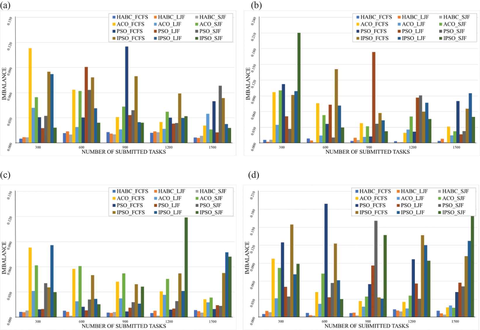
Degrees of load imbalance in a homogeneous environment when Heuristic Task Scheduling with Artificial Bee Colony (HABC), Ant Colony Optimization (ACO), Particle Swarm Optimization (PSO), and improved PSO (IPSO) were used with (a) datasets D1 - Random dataset, (b) datasets D4- Normal distribution dataset, (c) datasets D7- Random dataset with left-skewed distribution, (d) datasets D10 - Random dataset with right-skewed distribution.
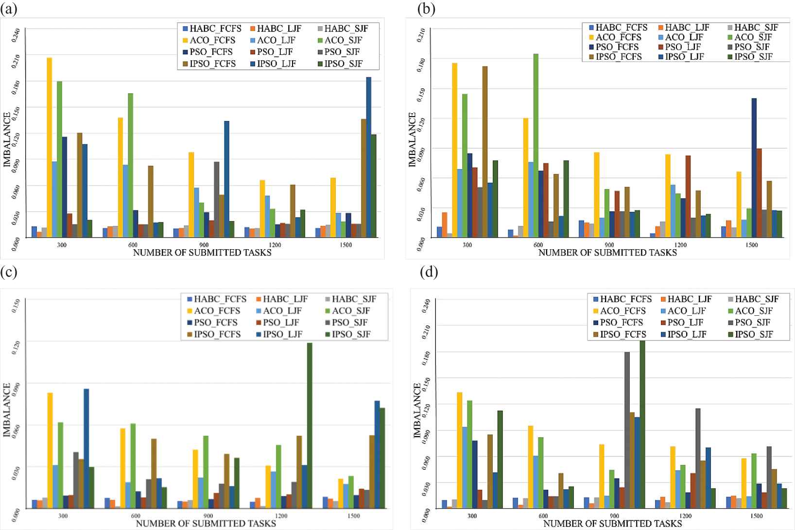
Degrees of load imbalance in a heterogeneous environment when Heuristic Task Scheduling with Artificial Bee Colony (HABC), Ant Colony Optimization (ACO), Particle Swarm Optimization (PSO), and improved PSO (IPSO) were used with (a) datasets D1 - Random dataset, (b) datasets D4- Normal distribution dataset, (c) datasets D7- Random dataset with left-skewed distribution, (d) datasets D10 - Random dataset with right-skewed distribution.
As shown in Figure 2, in order to consider the effect of different types of dataset on performance scalability of the system, we evaluated the average degrees of load imbalance with four datasets of different types: D1, D4, D7, and D10. The results show that the HABC algorithm (HABC_FCFS, HABC_LJF, HABC_SJF) performed lower average degrees of load imbalance than any of the compared algorithms (PSO and ACO algorithms) in the homogeneous environment.
In the same direction, the results in Figure 3 showed that the HABC algorithm (HABC_FCFS, HABC_LJF, HABC_SJF) outperformed the other two algorithms in the heterogeneous environment.
In the tuhird part, the performance of the HABC algorithm in terms of Standard Deviation (S.D.) was evaluated. In order to ensure that the tasks are equally distributed into VMs and the system is balanced workload.
We evaluated the S.D. with dataset D1 in Table 3. The number of groups of submitted tasks was varied in each run from 100 to 1500 submitted tasks in an increment of 100 tasks. The S.D. for 300, 600, 900, 1200, and 1500 tasks in cloud computing within homogeneous and heterogeneous environments are shown in Tables 12 and 13, respectively. Table 12 shows the S.D. of all tested algorithms with datasets (D1) in homogeneous environment. The results show that HABC algorithm has less S.D. values than other methods. In the same direction of heterogeneous environment in Table 13.
| Number of Tasks | HABC_FCFS | HABC_LJF | HABC_SJF | ACO_FCFS | ACO_LJF | ACO_SJF | PSO_FCFS | PSO_LJF | PSO_SJF | IPSO_FCFS | IPSO_LJF | IPSO_SJF |
|---|---|---|---|---|---|---|---|---|---|---|---|---|
| 300 | 0.12 | 0.06 | 0.09 | 1.09 | 1.01 | 1.12 | 0.51 | 0.38 | 0.46 | 0.21 | 0.14 | 0.16 |
| 600 | 0.11 | 0.05 | 0.08 | 2.07 | 2.03 | 2.09 | 0.51 | 0.38 | 0.45 | 0.21 | 0.14 | 0.15 |
| 900 | 0.09 | 0.04 | 0.07 | 3.02 | 2.99 | 3.04 | 0.48 | 0.37 | 0.44 | 0.18 | 0.13 | 0.14 |
| 1200 | 0.08 | 0.04 | 0.08 | 4.08 | 4.06 | 4.1 | 0.49 | 0.37 | 0.45 | 0.19 | 0.13 | 0.15 |
| 1500 | 0.09 | 0.07 | 0.09 | 5.05 | 5.03 | 5.06 | 0.52 | 0.36 | 0.44 | 0.22 | 0.12 | 0.14 |
HABC, Heuristic Task Scheduling with Artificial Bee Colony; ACO, Ant Colony Optimization; PSO, Particle Swarm Optimization; IPSO, improved PSO; FCFS, First Come First Serve; SJF, Smallest Job First; LJF, Largest Job First.
The comparison of Standard Deviation with HABC, ACO, PSO, and IPSO in a homogeneous environment with datasets D1.
| Number of Tasks | HABC_FCFS | HABC_LJF | HABC_SJF | ACO_FCFS | ACO_LJF | ACO_SJF | PSO_FCFS | PSO_LJF | PSO_SJF | IPSO_FCFS | IPSO_LJF | IPSO_SJF |
|---|---|---|---|---|---|---|---|---|---|---|---|---|
| 300 | 0.16 | 0.12 | 0.14 | 0.71 | 0.63 | 0.74 | 0.86 | 0.52 | 1.18 | 0.41 | 0.22 | 0.48 |
| 600 | 0.17 | 0.09 | 0.15 | 1.32 | 1.27 | 1.33 | 0.89 | 0.55 | 1.29 | 0.44 | 0.25 | 0.59 |
| 900 | 0.15 | 0.12 | 0.13 | 1.93 | 1.89 | 1.9 | 0.94 | 0.52 | 1.26 | 0.49 | 0.22 | 0.56 |
| 1200 | 0.17 | 0.13 | 0.12 | 2.57 | 2.56 | 2.59 | 0.87 | 0.53 | 1.03 | 0.42 | 0.23 | 0.33 |
| 1500 | 0.16 | 0.11 | 0.13 | 3.19 | 3.17 | 3.2 | 0.82 | 0.65 | 0.73 | 0.37 | 0.25 | 0.23 |
HABC, Heuristic Task Scheduling with Artificial Bee Colony; ACO, Ant Colony Optimization; PSO, Particle Swarm Optimization; IPSO, improved PSO; FCFS, First Come First Serve; SJF, Smallest Job First; LJF, Largest Job First.
The comparison of standard deviation with HABC, ACO, PSO, and IPSO in a heterogeneous environment with datasets D1.
The result of the experiment indicated that the makespan and the degree of imbalance are slight difference. On the other hand, if considered the performance measurement using S.D. between the HABC algorithm and ACO algorithm are very different. The results show that HABC algorithm highly enhanced the S.D. compared to the other algorithms in cloud computing within homogeneous and heterogeneous environments. The goal is to achieve a balance between the resources in the system and to minimize the makespan time.
To summarize, even though all of the presented algorithms utilize a similar scheduling process based on a heuristic method. When they were compared, the HABC algorithm was able to show a better performance than those shown by ACO, PSO, and IPSO algorithms, especially in the case of using large job submitting first (HABC_LJF). Moreover, the system still balanced the load of submitting tasks adequately with minimum makespan.
5. CONCLUSION
In this paper, to improve task scheduling and load balancing, an algorithm for VMs in cloud computing based on heuristic task scheduling called HABC for VMs in cloud computing within both homogeneous and heterogeneous environments is proposed. The HABC was implemented on a cloud computing model in order to optimize the process of task scheduling and load balancing of volumes of data. A detailed comparison between the performances of the proposed method and other compared algorithms including ACO algorithms, PSO algorithms, and improved PSO algorithms is also presented.
The experiments were conducted with four types of datasets in order to measure the performance of our algorithm in terms of minimum makespan, maximum makespan, average makespan, and degree of load imbalance. The results show that the HABC with Largest Job First heuristic algorithm (HABC_LJF) offers the best performance in scheduling and load balancing.
This novel-proposed approach can serve as a useful alternative for cloud computing within homogeneous and heterogeneous environments. However, this work was a simulation on a few datasets. In future works, we will further conduct similar experiments on larger datasets. We plan to apply this HABC method in other practical applications to real-world datasets and will explore the possibility of HABC to handle multiple job scheduling with different priorities.
COMPLIANCE WITH ETHICAL STANDARDS
CONFLICT OF INTEREST
The author declares that he has no conflict of interest against any company or institution.
ETHICAL STANDARDS
This research has not involved human participants and/or animals, except for the author contribution.
ACKNOWLEDGMENTS
Our appreciation goes to the Department of Computer Science, Faculty of Science, King Mongkut�s Institute of Technology Ladkrabang for supporting the facilities in doing this research.
REFERENCES
Cite this article
TY  - JOUR
AU  - Boonhatai Kruekaew
AU  - Warangkhana Kimpan
PY  - 2020
DA  - 2020/04/27
TI  - Enhancing of Artificial Bee Colony Algorithm for Virtual Machine Scheduling and Load Balancing Problem in Cloud Computing
JO  - International Journal of Computational Intelligence Systems
SP  - 496
EP  - 510
VL  - 13
IS  - 1
SN  - 1875-6883
UR  - https://doi.org/10.2991/ijcis.d.200410.002
DO  - 10.2991/ijcis.d.200410.002
ID  - Kruekaew2020
ER  -