
Online Streaming Feature Selection via Multi-Conditional Independence and Mutual Information Entropy†
- DOI
- 10.2991/ijcis.d.200423.002How to use a DOI?
- Keywords
- Streaming feature; Feature selection; Conditional independence; Mutual information
- Abstract
The goals of feature selection are to remove redundant and irrelevant features from high-dimensional data, extract the “optimal feature subset” of the original feature space to improve the classification accuracy, and reduce the time complexity. Traditional feature selection algorithms are based on static feature spaces that are difficult to apply in dynamic streaming data environments. Existing works, such as Alpha-investing and Online Streaming Feature Selection (OSFS), and Scalable and Accurate OnLine Approach (SAOLA), have been proposed to serve the feature selection with streaming feature, but they have drawbacks, including low prediction accuracy and a large number of selected features if the streaming features exhibit characteristics such as low redundancy and high relevance. To address the limitations of the abovementioned works, we propose the algorithm of Online Streaming Feature Selection via Conditional dependence and Mutual information (OSFSCM) for streaming feature, which is found to be superior to Alpha-investing and OSFS for datasets with low redundancy and high relevance. The efficiency of the proposed OSFSCM algorithm is validated through a performance test on widely used datasets, e.g., NIPS 2003 and Causality Workbench. Through extensive experimental results, we demonstrate that OSFSCM significantly improves the prediction accuracy and requires fewer selected features compared with Alpha-investing and OSFS.
- Copyright
- © 2020 The Authors. Published by Atlantis Press SARL.
- Open Access
- This is an open access article distributed under the CC BY-NC 4.0 license (http://creativecommons.org/licenses/by-nc/4.0/).
1. INTRODUCTION
Dimensionality reduction can combat the curse of dimensionality [1–4]. Feature selection chooses an “optimal feature subset” by following a certain criterion while removing redundant and irrelevant features of the class attribute during classification from the original high-dimensional feature set [2,5–7]. This process maintains relevant features for learning and provides faster and more cost-effective predictors with respect to efficiency and effectiveness [8].
In real-world applications, many datasets have very high-dimensional and increasing feature spaces [9,10], such as the datasets from the real-time monitoring and analysis of environments [11], capturing CCTV streaming images [12], collecting features for intrusion detection [13,14], real-time updates of popular topics in Microblog and Twitter [15,16], and real-time spam filtering of email [17]. In such streaming feature spaces, the new, individual features flow into the model dynamically and must be considered sequentially. As an emerging research direction during the past few years, online feature selection with streaming features offers a complementary algorithmic methodology to enrich online feature selection [9,18,19] that addresses high-dimensionality in big data analyses. This methodology assumes that sequential features flow into the model dynamically, and the feature selection is performed when features arrive. This approach is different from classical online learning in which the feature space remains consistent while samples flow in sequentially [19,20]. The representative classical methods [19] include Grafting, Alpha-investing, online streaming feature selection (OSFS), Online Feature Selection with Group Structure (OGFS), and scalable and accurate online approach (SAOLA).
Feature sets with a continuous flow of new features, such as in medical diagnosis, relevant features might be generated with low redundancy. This scenario results in many selected features being generated in the candidate feature set. Experiments from the previously mentioned studies demonstrate that feature selection is restricted in these datasets. For example, the Grafting algorithm is weak at handling streaming features because the entire feature space must be known. The algorithm of Alpha-investing has low prediction accuracy and is unstable. Although the OSFS algorithm offers high prediction accuracy for these types of datasets, the running time increases exponentially with increasing of selected features, so OSFS becomes very slow. The SAOLA algorithm offers good efficiency in its running time while having a few features, but its prediction accuracy is not excellent.
Motivated by the above analysis of existing studies of online feature selection with streaming features, we investigate the problem with a novel algorithm called Online Streaming Feature Selection via Conditional dependence and Mutual (OSFSCM) information to solve the following challenges: (1) how to select the feature subset in a streaming feature space with low redundancy and obtain high relevancy, (2) how to provide effective continuous mechanisms to discover the pattern of the running time among all generated features with increasing feature volumes, and (3) how to validate the performance.
The contributions of this paper that extend beyond the existing methods include our proposal of a novel algorithm for streaming feature selection, an analysis of its theoretical properties, and a validation of its empirical performance through extensive experiments.
The remainder of the paper is organized as follows: Section 2 surveys the related work and Section 3 introduces notations, definitions, and a framework for streaming feature filtering as well as the proposal of our OSFSCM algorithm and analysis. Section 4 reports our experimental results and describes its application in a real scenario, followed by our conclusion in Section 5.
2. RELATED WORK
Feature selection is simple, interpretable, and essential when working with high-dimensional data [18,19]. Based on the available label information, feature selection can include supervised, unsupervised, and semi-supervised methods. From the perspective of a selection strategy, these algorithms can include a wrapper, filter, or embedded method [19].
Online feature selection for streaming features is an important branch of feature selection [4,8,21] that focuses on scenarios where the number of features changes over time, which must be processed in real-time and not after all the features arrive. Representative algorithms of this field include Grafting, Alpha-investing, OSFS, OGFS, and SAOLA.
Grafting [22] is an embedded feature selection method applied to streaming features with irrelevant and redundant features. However, Grafting is weak for this approach because it must know about the entire feature space to select a good value for its regularization parameter. Alpha-investing [23] can handle infinitely large feature sets but also must transform the initial features based on prior knowledge of candidate features. Only judging the relevance of features can give many redundant features in the candidate set resulting in a reduction of classification accuracy. OSFS [24] uses the G2 test to denote conditional independence or dependence between features from which it identifies irrelevant and redundant features. While OSFS can remove these irrelevant and redundant features from streaming features, when the number of weak relevant features increases, the running time increases exponentially. OGFS [25] leverages the group structure information as a priori knowledge for feature selection and generates a better feature subset through two stages of intra-group and inter-group feature selection. However, OGFS must select a few parameters in advance, which is relatively difficult without prior information. SAOLA [15] can handle an extremely high-dimensional feature space by using a strategy of online pairwise comparisons. However, SAOLA only judges if the features are redundant under a single condition and cannot remove all redundant features. Besides, the algorithm alone cannot obtain the judgment threshold of the optimal relevance between features.
Based on the above observations, we propose an efficient OSFSCM algorithm for feature selection in a streaming feature space that offers low redundancy and high relevance.
3. THE OSFSCM ALGORITHM FOR ONLINE FEATURE SELECTION
3.1. Notations and Definitions
The selected features of the class attribute represent an optimal feature subset [24,26] containing all strongly relevant and nonredundant features [24], as shown in Figure 1. The optimal feature subset is named the Markov blanket of the class attribute, and this criterion only removes the attributes that are unnecessary for inclusion into the feature set because they are irrelevant or redundant [7,24,27]. We consider this problem in the context of online feature selection with streaming features where S is the feature space set containing all available features.
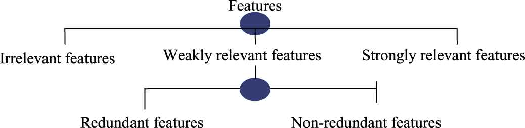
Feature relevance and redundancy [24].
Table 1 lists all symbols and notations used in this paper. Assume that xidenotes the ith new incoming feature at time ti, Si−1 is the selected feature set at time ti−1,
| Notation | Mathematical Meanings |
|---|---|
| S | Feature space set |
| f | Feature f, f ∈ S |
| CFS | Candidate feature set at current time |
| t | A time point |
| T | Class attribute |
| P(x) | Event probability of feature x |
| P(.|.) | Conditional probability |
| ρ | A threshold |
| MB(T) | Markov blanket of T |
| a |
a is independent of b |
Notations with mathematical meanings.
Definition 1 (Independence [28]).
In a set S, two variables x, y ∈ S are independent with respect to a probability distribution P, denoted as
Definition 2 (Conditional Independence [8]).
In a set S, two random variables x, y ∈ S are conditionally independent given a set of variables
Conditional independence is a generalization of the traditional notion of statistical independence in Bayesian networks due to the factorizations of the allowed joint probability distribution. If x and y are dependent in the condition of Si, then we write
Definition 3 (Markov blanket [15,29,30], MB).
A Markov blanket of the class attribute T, denoted as MB(T), is a minimal set of features that makes
MB(T) is the set of parents, children, and children's parents of T [31]. These Markov blankets can eliminate a conditionally independent feature without increasing the distance from the desired distribution. The Markov blanket criterion only removes the attributes that are unnecessary based on those that are irrelevant to the class attribute and redundant given other attributes [26].
Definition 4 (Strong relevance [24]).
A feature x is strongly relevant to the class attribute, T, iff
Definition 5 (Weak relevance [24]).
A feature x is weakly relevant to the class attribute, T, iff
Definition 6 (Irrelevance [24]).
A feature x is irrelevant to a class attribute, T, iff
Definition 7 (Redundant features [24]).
A feature x is redundant to the class attribute T iff it is weakly relevant to T and has a MB(x) that is a subset of MB(T).
3.2. Using Mutual Information to Filter Partial Redundant Features
Mutual information theory and Fisher's z-test are used to judge the correlation between features [15]. The evaluation standard of entropy information quantity, also known as Shannon entropy, uses a numerical value to express the uncertainty degree of a random variable. The entropy of feature Y is defined as
Conditional entropy refers to the uncertainty degree of another variable after it is known, i.e., the dependence degree of the variable on the known variable. Assuming the feature Z is known, the conditional entropy of Y under the Z condition is defined as
Conditional mutual information is the degree of correlation between two features under the condition that a certain feature is known. The expression of conditional mutual information is established according to Eqs. (3) and (4) [15].
When a new feature f arrives, to determine if it is relevant for the class attribute T, the algorithm calculates a correlation threshold δ, such that if I(f; T) > δ (0 ≤ δ ≤ 1), and
3.3. Using Fisher's z-Test to Filter Irrelevant and Partially Redundant Features with Continuous Data
Fisher's z-test calculates the correlation degree between features [15], as in shown in Eq. (5). In the Gaussian distribution N(μ, Σ), after the feature subset S is provided, the expression of the partial correlation coefficient
In Fisher's z-test, under the null hypothesis of the conditional independence between the feature fi and the class attribute T of the given feature subset S,
3.4. Using the G2 Test to Filter Irrelevant and Partially Redundant Features with Discrete Data
As an alternative to the X2 test, the G2 test is a statistic defined as Eq. (6) [24]
3.5. The OSFSCM Algorithm and Analysis
In this section, we propose a new approach for feature filtering via multi-conditional independence and mutual information entropy to process data with streaming features. In this approach, the data stream is fixed, while the features continue arriving as each feature is evaluated. The process of feature selection can be performed in three phase, as shown in Table 2. First, the irrelevant features are filtered by the nonconditional independence and leaving the relevant features. Second, part of the redundant features is further discarded from the weakly relevant features by filtering through mutual information. Finally, the remaining redundant features are discarded by filtering through conditional independence.
| Phase of Filtering | Feature Analysis |
|---|---|
| Phase1: filtering via nonconditional independence | Analysis of irrelevant features |
| Phase2: filtering via mutual information | Analysis of redundant features |
| Phase3: filtering via conditional independence |
Phase of filtering for streaming features.
According to the above approach, The OSFSCM algorithm for streaming feature filtering is proposed, as is shown in Algorithm 1.
Algorithm 1: The OSFSCM algorithm
Initialization
(1) Selected features set CFS = {}, class attribute T
Analysis of irrelevant features: filtering via non-conditional independence
(2) Get a new feature f;
(3) If f is an irrelevant feature, discard f, enter step (2);
(4) If not, CFS = CFS ∪ {f}, enter step 3;
Analysis of redundant features 1: the filtering via mutual information
(5)
Analysis of redundant features 2: the filtering via conditional independence
(6)
Repeat steps 2–5 until no new features or stopping criteria is met;
Output the selected features CFS.
In the OSFSCM algorithm, CFS is a candidate feature set at the current time, and f is the new feature. In step 2, nonconditional independence filtering is executed. If it returns an irrelevant feature of class attribute T, then the feature f is discarded. Otherwise, the feature f goes into further analysis of the redundant features.
The filtering of the redundant features is divided into two sequential steps. Step 3 includes the filtering via mutual information and step 4 filters via conditional independence.
For filtering via mutual information, according to Eq. (4), a new feature f is relevant with T,
For filtering via conditional independence, the candidate feature set CFS includes the new feature f, and the expression of
The OSFSCM uses the notation
3.6. The Time Complexity of OSFSCM
The complexity of the OSFSCM algorithm depends on the tests of nonconditional independence filtering, mutual information filtering, and conditional independence filtering. Assume that |N| is the number of features arrived, and |N| also is the number of remaining features before filtering via non-conditional independence, |S1| is the number of remaining features before filtering via mutual information, and |CFS| is the number of remaining features before filtering via conditional independence. For OSFSCM, we use the k-greedy search strategy with k = 3. The complexity of each filtering phase is shown in Table 3. Therefore, the complexity is represented as
| Phase of filtering | Cost |
|---|---|
| Phase1: filtering via nonconditional independence | O(|N|) |
| Phase2: filtering via mutual information | O(|S1||CFS|) |
| Phase3: filtering via conditional independence |
OSFSCM, online streaming feature selection via conditional dependence and mutual information.
The time complexity of OSFSCM algorithm.
4. EXPERIMENTAL RESULTS
4.1. Experiment Setup
We empirically evaluate the performance of the OSFSCM algorithm on 14 benchmark datasets listed in Table 4. All experiments are performed on a computer with an Intel(R) Xeon(R) CPU E3-1505M 3.0 GHz with 32 G RAM.
| Dataset | #Features | #Instances |
|---|---|---|
| wdbc | 30 | 569 |
| colon | 2000 | 62 |
| lucas0 | 11 | 2000 |
| sylva | 216 | 13086 |
| ionosphere | 34 | 351 |
| cina0 | 132 | 16033 |
| lucap0 | 143 | 2000 |
| marti1 | 1024 | 500 |
| reged1 | 999 | 500 |
| lung | 3312 | 203 |
| prostate_GE | 5966 | 102 |
| leukemia | 7066 | 72 |
| arcene | 10000 | 100 |
| Smk_can_187 | 19993 | 187 |
#Features: the number of features; #Instances: the number of instances.
The benchmark datasets used for algorithm evaluation.
The arcene, colon, ionosphere, and leukemia datasets are sourced from the NIPS 2003 feature selection challenge [8] and a frequently studied public microarray datasets (wdbc). We also downloaded the datasets from the Causality Workbench that includes sylva, lung, cina0, reged1, lucas0, marti1, and lucap0. The cina0 is a marketing dataset derived from census data. The reged1 is a genomics dataset for studying the causes of lung cancer. The marti1 is obtained from the data generative process of simulated genomic data. The lucas0 is a lung cancer simple set, and lucap0 is a lung cancer set with probes, which are used for modeling a medical application for the diagnosis, prevention, and cure of lung cancer. The number of features available in these datasets ranges from 11 to 10000, and the number of samples varies from 72 to 145252. In particular, the number of features of seven datasets is larger than the number of samples, including marti1, reged1, lung, prostate_GE, leukemia, arcene, and Smk_can_187. These 14 datasets cover a wide range of real-world application domains, including gene expressions, ecology, and casual discovery, making the construction of feature selection very challenging. We preprocess the data by turning to a standard score and deleting the same columns, such as in leukemia and other datasets.
Our analysis of the OSFSCM algorithm compares against the state-of-the-art online feature selection algorithms, Alpha-investing, and OSFS, using 10-fold cross-validation on each training dataset. First, we compared the prediction accuracy of OSFSCM with that of the state-of-the-art using 12 classifiers, including Decision Tree, KNN, SVM, and Ensemble, as implemented in MATLAB. Second, we analyzed the number of selected features and the running time for each algorithm. Third, the OSFSCM algorithm is applied to a real-world data scenario and compared with the other algorithms.
4.2. Comparison of OSFSCM with Two Online Algorithms
The algorithms are implemented in Library of Online Streaming Feature Selection (LOFS) [18], an open-source library available in MATLAB 2017. To evaluate the selected features in the experiments, we use twelve available classifiers in the app of “classification learner” in MATLAB 2017, including Decision Trees (Complex Tree, Medium Tree, and Simple Tree), SVM (Linear, Quadratic, and Cubic), KNN (Fine, Medium, and Cubic), and Ensemble (Bagged Trees, Subspace discriminant, and RUSBoosted Trees) classifiers. In the app of classification learner, we automatically train these classification models with default parameters, as is shown in the Table 5. We choose the results of OSFSCM, OSFS, and Alpha-investing as the datasets to train and validate classification models. After training multiple models, compare these algorithms' performance side-by-side in these classifiers.
| Classifier Parameters | Parameter Values |
||
|---|---|---|---|
| Complex Tree | Medium Tree | Simple Tree | |
| Maximum number of splits | 100 | 20 | 10 |
| Split criterion | Gini's diversity index | ||
| Surrogate decision splits | Off | ||
| Maximum surrogates per node | 10 | ||
| Linear SVM | Quadratic SVM | Cubic SVM | |
| Kernel function | Linear | Quadratic | Cubic |
| Box constraint level | 1 | ||
| Kernel scale mode | Auto | ||
| Manual kernel scale | 1 | ||
| Fine KNN | Medium KNN | Cubic KNN | |
| Number of neighbors | 1 | 10 | 10 |
| Distance metric | Euclidean | Euclidean | Minkowski |
| Distance weight | Equal | ||
| Box constraint level | 1 | ||
| Kernel scale mode | Auto | ||
| Manual kernel scale | 1 | ||
| Bagged Trees | Subspace Discriminant | RUSBoosted Trees | |
| Ensemble method | Bag | Subspace | RUSBoost |
| Learner type | Decision tree | Discriminant | RUSBoost |
| Maximum number of splits | 266 | 20 | 20 |
| Number of learners | 30 | ||
| Learning rate | 0.1 | ||
| Subspace dimension | 1 | ||
Parameter settings in 12 classifiers.
As described above, we evaluate OSFSCM against the others based on prediction accuracy, the number of selected features, and the running time. In the following, we perform statistical comparisons to analyze the prediction accuracies further.
4.2.1. Prediction Accuracy
Figure 2 summarizes the prediction accuracies with 12 classifiers applied to 14 datasets during online learning. We conduct these tests using G2 for discrete data and Fisher's z-test for continuous data at an α = 0.05 significance level. The prediction accuracies of OSFSCM and OSFS are higher compared with Alpha-investing for most of the 5–14 datasets for these classifiers. OSFSCM achieves a higher accuracy for all the classifiers except for RUSBoosted Trees. With some datasets, as seen in Figure 2, the accuracies of the classifiers are reduced too much, such as in leukemia, marti1, and reged1.
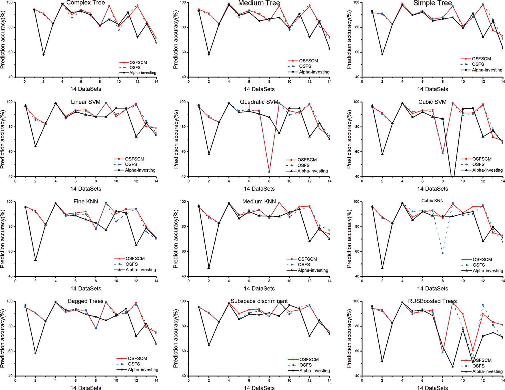
Prediction accuracies of the three algorithms on 14 datasets using classifiers on the selected features. The x-axis labels represent the 14 datasets as (1) wdbc, (2) colon, (3) lucas0, (4) sylva, (5) ionosphere, (6) cina0, (7) lucap0, (8) marti1, (9) reged1, (10) lung, (11) prostate_GE, (12) leukemia, (13) arcene, and (14) Smk_can_187.
In addition, from the three curves in Figure 2, the prediction accuracies from Alpha-investing, OSFS, and OSFSCM are nearly the same for some datasets, including six datasets using Complex Tree, three each using Medium Tree, Liner SVM, Quadratic SVM, Cubic SVM, Fine KNN, Medium KNN, and Subspace discriminant, two datasets with Cubic KNN, Bagged Trees, and RUSBoosted Trees, and one dataset with Simple Tree. For the wdbc, lucas0, and sylva datasets, the prediction accuracies of these classifiers, as well as RUSBoosted Trees, remain nearly the same.
4.2.2. Number of Selected Features and Running Time
To further examine these three algorithms, Table 6 lists the performance of each with respect to the 14 datasets comprised of different numbers of features.
Summary of the numbers of selected features
While the prediction accuracy of OSFSCM is higher than Alpha-investing and OSFS for most datasets, as previously described in Figure 2, another observation is apparent in Table 6. The number of selected features from OSFSCM is more than Alpha-investing and OSFS for many datasets. This result is due to the following reasons:
For the Alpha-investing algorithm: From its low prediction accuracy, the ability of the algorithm to mine features is low, so part of the Markov blanket elements cannot be obtained.
For the OSFS algorithm: During the redundant feature analysis phase, the non-redundant features could be discarded under the condition of redundant features due to its low prediction accuracy, so fewer features are selected.
For the OSFSCM algorithm: A large number of selected features is potential due to its significant outperformance over OSFS and Alpha-investing in mining the elements from the Markov blanket, enabling it to find more elements.
Summary of the running times
The running time performances for the three algorithms are also reported in Table 6. The Alpha-investing is faster than OSFS and OSFSCM for all datasets because it only considers the newest feature added, and never considered the discarded features again. This approach also results in low prediction accuracy (as seen in Figure 2) with the classifiers, as with the datasets colon, lucap0, reged1, leukemia, and Smk_can_187.
The performances of the running times in OSFSCM and OSFS are very different, as seen in the results in Table 6, with OSFS being much faster than OSFSCM on the datasets of wdbc, colon, lucas0, ionosphere, lung, prostate_GE, arcene, leukemia, and Smk_can_187.
On the other hand, OSFSCM is much faster compared with OSFS on the datasets of sylva, cina0, lucap0, reged1, and lung, as highlighted in bold. These datasets include features with higher feature selection, as shown in Table 4, and have low redundancy with high strong and weak relevance because the number of candidate features significantly influences the runtime for the two algorithms.
| Dataset | Alpha-Investing |
OSFS |
OSFSCM |
|||
|---|---|---|---|---|---|---|
| #Features | Time(s) | # Features | Time(s) | # Features | Time(s) | |
| wdbc | 20 | 0.0138 | 3 | 0.1577 | 3 | 0.0567 |
| colon | 1 | 0.0663 | 3 | 0.6778 | 4 | 0.0582 |
| lucas0 | 4 | 0.0008 | 4 | 0.0142 | 4 | 0.0061 |
| sylva | 70 | 1.6717 | 18 | 247.9366 | 22 | 32.5611 |
| ionosphere | 10 | 0.0147 | 4 | 0.1315 | 7 | 0.0669 |
| cina0 | 8 | 0.1046 | 22 | 721.3638 | 28 | 62.1947 |
| lucap0 | 10 | 0.0197 | 36 | 1.43E+07 | 41 | 72.5523 |
| marti1 | 28 | 0.116 | 1 | 0.1081 | 1 | 0.1045 |
| reged1 | 1 | 0.0417 | 13 | 121.2839 | 13 | 27.3695 |
| lung | 45 | 0.7523 | 11 | 420.5678 | 20 | 85.3698 |
| prostate_GE | 12 | 0.4308 | 3 | 7.7915 | 4 | 3.1189 |
| leukemia | 1 | 0.4346 | 3 | 12.7647 | 5 | 8.3657 |
| arcene | 8 | 1.4139 | 5 | 20.8445 | 6 | 5.8624 |
| Smk_can_187 | 6 | 2.7929 | 4 | 42.8323 | 7 | 12.1648 |
OSFS, online streaming feature selection; OSFSCM, online streaming feature selection via conditional dependence and mutual information.
Number of selected features and running time.
4.3. Application in a Real Scenario
The PEMS-SF dataset from the UCI website is selected for our real scenario test for algorithm evaluation. This dataset contains 440 instances and 138672 features based on 963 sensors recordings between January 1, 2008, and September 30, 2009, of daily lane occupancy rates on highways. Each feature represents a lane occupancy rate from a sensor for a day (between 0 and 1) with a classification label of 1 through 7, representing Monday to Sunday. The dataset deleted data on public holidays and anomalies observed on March 8 and March 9, 2008. This evaluation only considers the OSFSCM, OSFS, and SAOLA algorithms because the Alpha-investing algorithm cannot run in the PEMS-SF dataset. The significance level α is set to 0.05, and the experiment performs multiple 10-fold cross-validations.
Table 7 reports the running time of the OSFSCM algorithm on the PEMS-SF dataset. As the features flow in, OSFSCM removes many irrelevant and redundant features. First, irrelevant features can be removed by the filtering of nonconditional independence, followed by the removal of redundant features by the filtering of mutual information and conditional independence. Finally, the approximate Markov blanket of the classification label is obtained by the three filters.
| Algorithm | Time(s) | #Features |
|||
|---|---|---|---|---|---|
| Ratio (%) | % Filtering via Nonconditional Independence | Filtering via Mutual Information | Filtering via Conditional Independence | ||
| OSFSCM | 476.3568 | 25 | 14295 | 98 | 21 |
| 50 | 31461 | 110 | 33 | ||
| 75 | 46636 | 150 | 35 | ||
| 100 | 61618 | 210 | 41 | ||
OSFSCM, online streaming feature selection via conditional dependence and mutual information.
Running time and the number of selected features from OSFSCM algorithm.
Compared with the low prediction accuracy of Alpha-investing and a high running time cost (greater than three days) of OSFS on the PEMS-SF dataset, OSFSCM and SAOLA complete the dataset filtering with many instances and features in a limited time. As is shown in Figure 3, the classification accuracies of OSFSCM on Decision Tree (simple tree), SVM (qualitative SVM), KNN (cosine KNN), and embedded (bagged trees) are higher compared with SAOLA, with differences of 8.63%, 3.11%, 10.03%, and 2.81%, respectively.
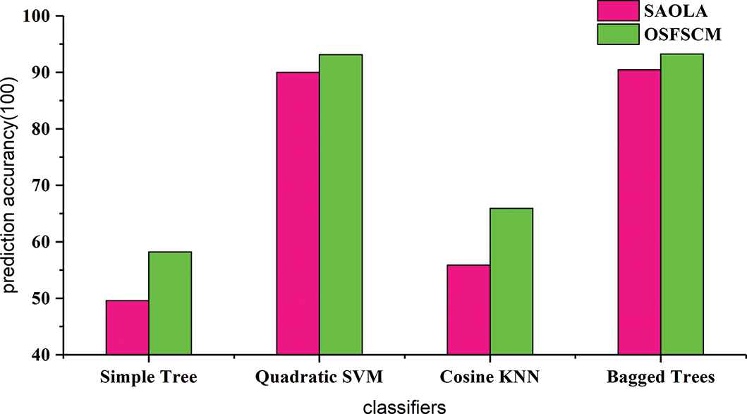
Classification accuracies on the PEMS-SF dataset using four classifiers.
5. CONCLUSIONS
We explored OSFS through a proposed algorithm called OSFSCM designed with conditional dependence and mutual information. Using benchmark datasets, we compared the OSFSCM algorithm with two state-of-the-art online feature selection methods, and our empirical results demonstrated the following: (1) The prediction accuracy of OSFSCM is higher compared with Alpha-investing and OSFS for many datasets. (2) The efficacy of the OSFSCM algorithm is high for these datasets, especially those with low redundancy and high relevance. (3) The number of selected features from OSFSCM is greater compared with Alpha-investing and OSFS for many datasets. (4) The validity of the OSFSCM algorithm is verified by tests using a real-world dataset scenario.
CONFLICT OF INTEREST
The authors declare they have no conflicts of interest.
AUTHORS' CONTRIBUTIONS
Hongyi Wang: conceptualization, validation, investigation, resources; Dianlong You: methodology, formal analysis, writing—original draft, data curtain, writing—review and editing, supervision.
Funding Statement
The National Natural Science Foundation of China under grant No.61772450, China Postdoctoral Science Foundation Grant under grant No.2018M631764, Hebei Natural Science Foundation under grant No.F2017203307, Hebei Postdoctoral Research Program under grant No.B2018003009, and the Doctoral Fund of Yanshan University under grant No.BL18003.
ACKNOWLEDGMENTS
The authors would like to thank the anonymous reviewers for their valuable comments and suggestions to improve the quality of the article.
Footnotes
The National Natural Science Foundation of China under grant No.61772450, China Postdoctoral Science Foundation Grant under grant No. 2018M631764, Hebei Natural Science Foundation under grant No. F2017203307, Hebei Postdoctoral Research Program under grant No. B2018003009, and the Doctoral Fund of Yanshan University under grant No. BL18003.
REFERENCES
Cite this article
TY  - JOUR
AU  - Hongyi Wang
AU  - Dianlong You
PY  - 2020
DA  - 2020/05/06
TI  - Online Streaming Feature Selection via Multi-Conditional Independence and Mutual Information Entropy†
JO  - International Journal of Computational Intelligence Systems
SP  - 479
EP  - 487
VL  - 13
IS  - 1
SN  - 1875-6883
UR  - https://doi.org/10.2991/ijcis.d.200423.002
DO  - 10.2991/ijcis.d.200423.002
ID  - Wang2020
ER  -