
Multi-view Genetic Programming Learning to Obtain Interpretable Rule-Based Classifiers for Semi-supervised Contexts. Lessons Learnt
 , Sebastián Ventura
- DOI
- 10.2991/ijcis.d.200511.002How to use a DOI?
- Keywords
- Multi-view learning; Rule-based classification; Comprehensibility; Semi-supervised learning; Co-training; Grammar-based genetic programming
- Abstract
Multi-view learning analyzes the information from several perspectives and has largely been applied on semi-supervised contexts. It has not been extensively analyzed for inducing interpretable rule-based classifiers. We present a multi-view and grammar-based genetic programming model for inducing rules for semi-supervised contexts. It evolves several populations and views, and promotes both accuracy and agreement among the views. This work details how and why common practices may not produce the expected results when inducing rule-based classifiers under this methodology.
- Copyright
- © 2020 The Authors. Published by Atlantis Press SARL.
- Open Access
- This is an open access article distributed under the CC BY-NC 4.0 license (http://creativecommons.org/licenses/by-nc/4.0/).
1. INTRODUCTION
In semi-supervised learning [1,2], given a set with a few labeled samples and a large collection of unlabeled ones, the goal is to infer a function that describes the relation between some inputs and a desired output and that the error associated to that function be lower to that for another inferred from just the labeled samples.
Multi-view learning [3,4], which has been widely applied to semi-supervised contexts [5,6], is a new machine learning paradigm that intends to obtain better results by training multiple functions, instead of considering just one of them. Multi-view learning mainly relies on two principles that ensure its success: the consensus principle, which says that minimizing the disagreement among the views reduces their individual error rates, and the complementary principle, that states that each view may contain some knowledge that other views lack.
Multi-view learning is often connected with multi-source learning [7], where the relevant information comes from different sources (such as text, audio, images, web addresses…). In such cases, independent functions are usually induced from each source and the best from the joint interaction is searched. However, the multi-view approach has also been applied successfully on single-source contexts [8–13], where the joint learning processes of multiple functions may cooperate to produce better single target functions. For this reason, views are better understood as the result of the input-learner pair. On the other hand, it is also related with ensembles [14,15], where multiple functions collaborate to produce better results. But the product of the multi-view methodology does not need to be an ensemble. In particular, since the multi-view learning approach assumes that the joint training reduces the individual error rates of the views, each of them is benefited from the learning process of the other views; so each single view becomes a candidate target function for the machine learning problem, potentially better than a function induced according to a single-view methodology.
Rule-based systems [16] are a representation paradigm that models knowledge by means of IF-THEN rules. In the context of supervised learning, the IF part, or antecedent, defines attribute conditions that patterns must satisfy in order to be covered by the rule; whereas the THEN part, or consequent, predicts the class of these covered patterns. One of the major benefits of rule-based systems, in contrast to other machine learning tools, is their comprehensibility, because rules are easily interpretable for experts in the addressed problems [17–21]. Notice here that one particularity of rule-based systems is that they define their own set of attributes whose decisions are based on. This means that they define particular views for analyzing the input information, with either empty or nonempty intersections. Therefore, multiple-induced rule-based systems are precisely subject of the multi-view approach, where the joint learning may produce better single systems even from the same dataset. A widely applied search paradigm to induce rule-based classifiers is genetic programming [22–24]. It applies the biological evolutionary metaphor on individuals that represent classification rules to generate robust classifiers.
In this work, our intention is to take advantage of the multi-view paradigm to get a single base classifier built on interpretable rules for semi-supervised contexts. Thus, our work is distinguished from (1) multi-source learning, because it can be applied on single-source cases, from (2) the ensembles practice, because the goal is to get a single base classifier, not a compound, and (3) other works about rule induction for semi-supervised contexts based on self-training [25,26], which promote a (single-view) reinforcement learning on the own most confident predictions for unlabeled patterns. In addition, we shall mention that there are not, to our knowledge, published works combining the multi-view approach exploiting the consensus principle with the task of inducing rule-based classifiers, except for a preliminary study [27] of ours.1 This article describes the peculiarities that this endeavor has introduced, given that the considered common practices did not promote the expected results. Concretely, our study suggests that
The multi-view learning approach, as expected, may really allow the learning process to take advantage of the presence of unlabeled patterns to induce, although very slightly and without large statistical differences, better rule-based classifiers.
The number of views slows down the convergence toward good classifiers, because having more views introduces more noise into the consensus-based co-training process. In our case, our model with just two views offered the best results.
Contrary to most approaches exploiting the consensus principle, which apply a linear combination between the accuracy on labeled patterns and the agreement among the views for unlabeled ones, our model with a lexicographic aggregation scheme attained the best performance scores. We are aware that this scheme assumes that training samples are never incorrectly labeled. In our case, the linear combination was allowing that wrong predictions of some views were learnt by other views, which increases the agreement among views at the expense of an inferior accuracy on the labeled patterns.
Though most rule-based systems incorporate a default rule for uncovered patterns, its corresponding predictions should be avoided when promoting the agreement among the views (the learning stage). This is due to these predictions are unreliable and may probably mislead other views. However, its usage in testing and production stages is necessary to get good results.
Imposing a diverse search among the different views, in an attempt to get some benefits from the complementary principle, probably makes difficult to get a good single classifier.
The article is structured as follows: In Section 2, we revise the concepts of multi-view learning and grammar-based genetic programming relevant to our study. In Section 3, our model for inducing interpretable rule-based classifiers under the multi-view paradigm is detailed. In Section 4, the experiments carried out, supporting the aforementioned conclusions, are presented. Finally, Section 5 gives an account of our conclusions and future works.
2. BACKGROUND
2.1. Multi-view Learning
In most data analytic problems, the information is collected from multiple sources, such as audio and video for video surveillance, words, title and headings, and citation references for bibliography studies, etc. In these cases, the variables of each sample are naturally partitioned into groups, which correspond to particular descriptions of the same sample. In contrast to classical methodologies for machine learning, which would intend to infer a single function from the concatenation of the variable groups, the multi-view paradigm attempts to improve the learning performance by exploiting the redundant descriptions of the same samples. To reach this goal, this approach produces a function for each group of variables, a view, and expects the joint optimization of all the views to generate a better result.
Multi-view learning mainly relies on three assumptions, namely, sufficiency, each view is sufficient to infer the target function on its own, compatibility, target functions of different views predict the same label from the descriptions of the same sample with a high probability, and conditional independence, views are conditionally independent given the label [3,4]. Having assumed these or some weaker properties, most proposals exploit the following two principles:
Consensus principle: Its goal is to maximize the agreement among the views. It is proved that, under soft assumptions, minimizing the disagreement among the views expectedly reduces the error rate of each of them [28]. Therefore, many multi-view approaches addressing semi-supervised problems intend to minimize the error on labeled examples and maximize the agreement on unlabeled ones. This methodology is known as co-training [29,30], which, in case of two views, tries to minimize the following, or another similar, equation (Eq. (1) in Ref. [4]):
where the first term refers to the agreement between the views on unlabeled examples (Complementary principle: It says that each view may contain some knowledge that other views have not, and then, multiple views can comprehensively describe the data. This principle, in conjunction with the consensus one, is usually exploited as follows: one view might have sufficient knowledge to accurately label an unlabeled example, which other views cannot classify with the same certainty; then, this example, with the predicted label, becomes part of the training set of the other views. This way, views exchange complementary information and learn in cooperation [11,31].
Even though multi-view approaches are naturally suitable for multi-source contexts, as described above, some researchers have analyzed its benefits when applied on single-source data. In Ref. [11], two views are trained on the same single-source dataset and it is shown that initial larger disagreements, even with different base learners, may allow final greater improvements. In Ref. [12], Wang et al. propose a multiviewization procedure for single-source datasets, based on reshaping the array of attributes into matrices with suitable dimensions, and present the results of a multi-view approach with regard to its corresponding single-view addressing. In this case, the number of attributes determines the maximum number of compatible matrices, and thus, the maximum number of views. As another example, kernel functions, such as the linear, polynomial, and the Gaussian kernels, define different similarity notations on the attribute space, so kernels may naturally correspond to different ways to describe the information [4]. This has encouraged some authors to search for the optimal combination of these kernel functions, in a multiple kernel learning fashion, even on single-source data [32,33].
For many other examples of multi-view approaches, on either multiple or single-source contexts, the interested reader is referred to the specialized surveys on multi-view and multi-source learning [3,4,34].
2.2. Grammar-Based Genetic Programming for Classification Rule Induction
Genetic programming simulates the principle of natural selection to evolve computer programs [35]. As all evolutionary algorithms do, genetic programming maintains a population of individuals, which represent candidate solutions for the problem at hand. In each generation, individuals are selected, crossed over, and mutated to produce new ones. The quality of the individuals is evaluated by the objective function, which assesses their abilities to solve the problem. Then, their quality values are used to promote the selection of the best individuals. Hence, the biased production of new candidate solutions foments that the quality of the individuals in the population improves throughout the generations.
The main difference between genetic programming and other evolutionary algorithms is the way candidate solutions are encoded, trees, as they are suitable to represent computer programs. In these trees, internal nodes are functions and leaf nodes are terminal symbols. In case of searching for classification rules, individuals encode IF-THEN rules with an antecedent and a class prediction as consequent. The antecedent contains a logical formula, with conditions on the attributes' values, that patterns must satisfy to be covered by the rule. Figure 1 shows an example of an antecedent that covers patterns whose first attribute is less or equal to two and the fourth one is not equal to “b”
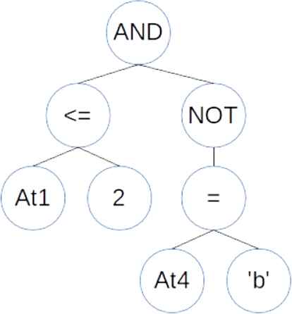
A tree representing the antecedent of an IF-THEN rule.
In general, individuals' antecedents are mutated and crossed over according to some probabilities, whereas their consequents are set externally or by an heuristic procedure [36], as the one described in Section 3.1. Mutation usually changes the value of, or generates a new subtree from, a randomly chosen node; and recombination exchanges two randomly selected subtrees of two individuals. However, these operators may produce invalid individuals if the closure property is not guaranteed [35], i.e., if some functions require operands of a certain type (numbers, categorical values, logical values…), and might be combined with operands of another one.
Grammar-based genetic programming [37–39] is an approach for ensuring that generated individuals always represent valid formulas by using a predefined grammar, such as that presented in Figure 2. In summary, the individuals of the initial population are generated by selecting random derivation rules for the nonterminal symbols they have, starting with the initial symbol (<antecedent> in Figure 2), mutation modifies nodes or subtrees according to their corresponding derivation rules, and recombination selects nodes in parents that were produced by the same or compatible production rules.
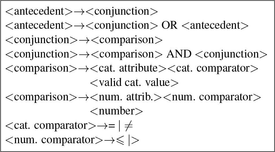
An example of a grammar for the antecedent of IF-THEN rules.
3. A MULTI-VIEW GENETIC PROGRAMMING MODEL FOR RULE-BASED SEMI-SUPERVISED LEARNING
This section describes our proposal of a grammar-based genetic programming algorithm for multi-view rule-based learning. Section 3.1 describes the base model our proposal is built on, which is a grammar-based genetic programming model for inducing rule-based classifiers in single-view fully supervised contexts. Section 3.2 details the adaptations introduced to carry out a multi-view learning for semi-supervised contexts.
3.1. A Grammar-Based Genetic Programming Algorithm for Supervised Classification Rule Induction
Bojarczuk et al presented a grammar-based genetic programming algorithm to induce good rule sets for supervised learning [36]. The model is an evolutionary algorithm whose individuals consist of an antecedent, a set of conditions connected by logical operators, and a consequent, which is the predicted class for the patterns that satisfy the antecedent. The antecedent of each individual is encoded as a tree where internal nodes represent either a logical or a conditional operator (numeric or categorical), and leaf nodes may take either pattern attributes or constant values. The initial generation of the antecedents of the individuals and the crossover operator ensure that antecedents are generated according to the grammar in Figure 2 (no mutation was considered), where <cat. attribute> and <num. attribute> refer to a pattern feature, and <valid categorical value>, to a possible value of the previously selected categorical attribute.
The consequent is not determined until the individual undergoes evaluation, when the quality of the rule is evaluated for each class of the problem, and the one that maximizes its fitness value is chosen. In particular, the sensitivity (2) and specificity (3) of the rule, on the training set
The algorithm evolves the population of individuals, maintaining an elite rule for each class of the problem throughout the generations (Figure 3):
First, the antecedent of the individuals are randomly generated. At this moment, individuals have not got any associated consequent nor fitness value, and the elite population is empty.
The individuals of the population are evaluated according to the aforementioned procedure, which assigns a consequent and a fitness value to each of them.
For each class of the problem, the best individual whose consequent is that class, if that has ever been generated, is stored in the elite set.
The whole population, elite and nonelite individuals, undergoes selection, crossover and reproduction to generate new individuals. Notice that the elite set is directly copied into the new population.
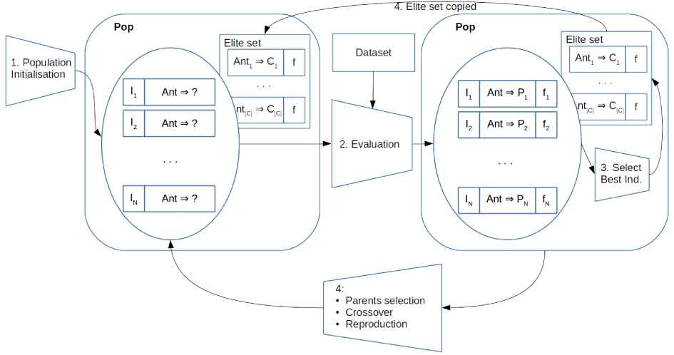
Grammar-based genetic programming approach for rule-based classification.
At the end, elite individuals conform the induced rule-based classifier.
3.2. A Multi-population Approach for Multi-view Learning
We have extended the previous model to exploit the consensus principle of the joint co-training of multiple views, obtaining a multi-view approach for semi-supervised learning. The main idea is to consider multiple subpopulations that evolve independently, each carrying out the learning process of a view over the same data, but cooperating to correctly identify the potential class of unlabeled patterns.
The key element in this model is the evaluation of the individuals of the populations, which considers both the success when predicting the class of labeled patterns and the agreement when predicting the label of unlabeled ones. Thus, individuals are associated with two performance measures, which are considered when they are selected to produce new offspring: the product of the sensibility and specificity of each rule according to (1) the labeled patterns, and (2) the predictions of the other views on the unlabeled samples, which are obtained according to their respective elite rule sets. Once these two performance measures have been computed for every individual, populations undergo evolution independently, i.e., selection and genetic operators are applied on each one to generate new individuals, which are again evaluated as described above.
In details, our model executes the following operations:
At the beginning, the individuals of the populations are randomly generated as in the first step of Figure 3. These initial individuals are evaluated just according to their success on the labeled patterns (
Each population selects its best individuals, one per class of the problem, if they exists, to conform its elite rule set (third step of Figure 3).
The parents for generating new individuals are selected according to an aggregation of their success on the labeled patterns (
Parents are crossed over according to a given probability, otherwise they are copied into the offspring, and offspring are mutated according to the mutation probability. Contrary to the proposal in Ref. [36], we apply the usual mutation operator commented in Section 2.2.
Once new individuals have been generated, they undergo evaluation (Figure 4).
At the beginning of the evaluation step, the consequents of the individuals and their fitness information is absent. The only information preserved from the previous iteration consists of the elite rules and their corresponding prediction success on the labeled patterns. Note that their
In the first phase, the accuracy of new individuals on the labeled patterns is computed. This phase assigns their
In the second phase, unlabeled patterns are first classified according to the elite rules of every view. This produces view-input-prediction triples, from which input-prediction pairs are used for computing the agreement according to the sensitivity and specificity equations. View-input-prediction triples of the own view are discarded to avoid the undesired and biased reinforcement. This way, elite and nonelite individuals get their
Notice that this one-triple-one-pair approach implicitly regulates the confidence on the predictions for unlabeled patterns with regard to other approaches such as, for instance, the majority vote. As an example, let us assume that we get the predictions
Finally, the elite population is updated with the best individual for each class. To carry out this selection, the same aggregation between the prediction success and consensus values, considered for parents selection, is applied. Note that elite rules may be replaced by new individuals, if the aggregation measure of these latter are better, which may be due to a higher prediction success on labeled patterns and/or a higher agreement with the predictions of the other views on the unlabeled samples.
Then, steps 3-5 are repeated until the stop condition is reached. The result is the elite set of any view, to which a default classification rule is appended. Section 4.4 analyzes the importance of this default rule. Notice that, although we could construct an ensemble with the elite sets of all the views, the output is just one of them (randomly selected), because we are interested in obtaining an interpretable classifier, i.e., the multi-view co-training approach is followed just to get a better but single rule-based classifier.
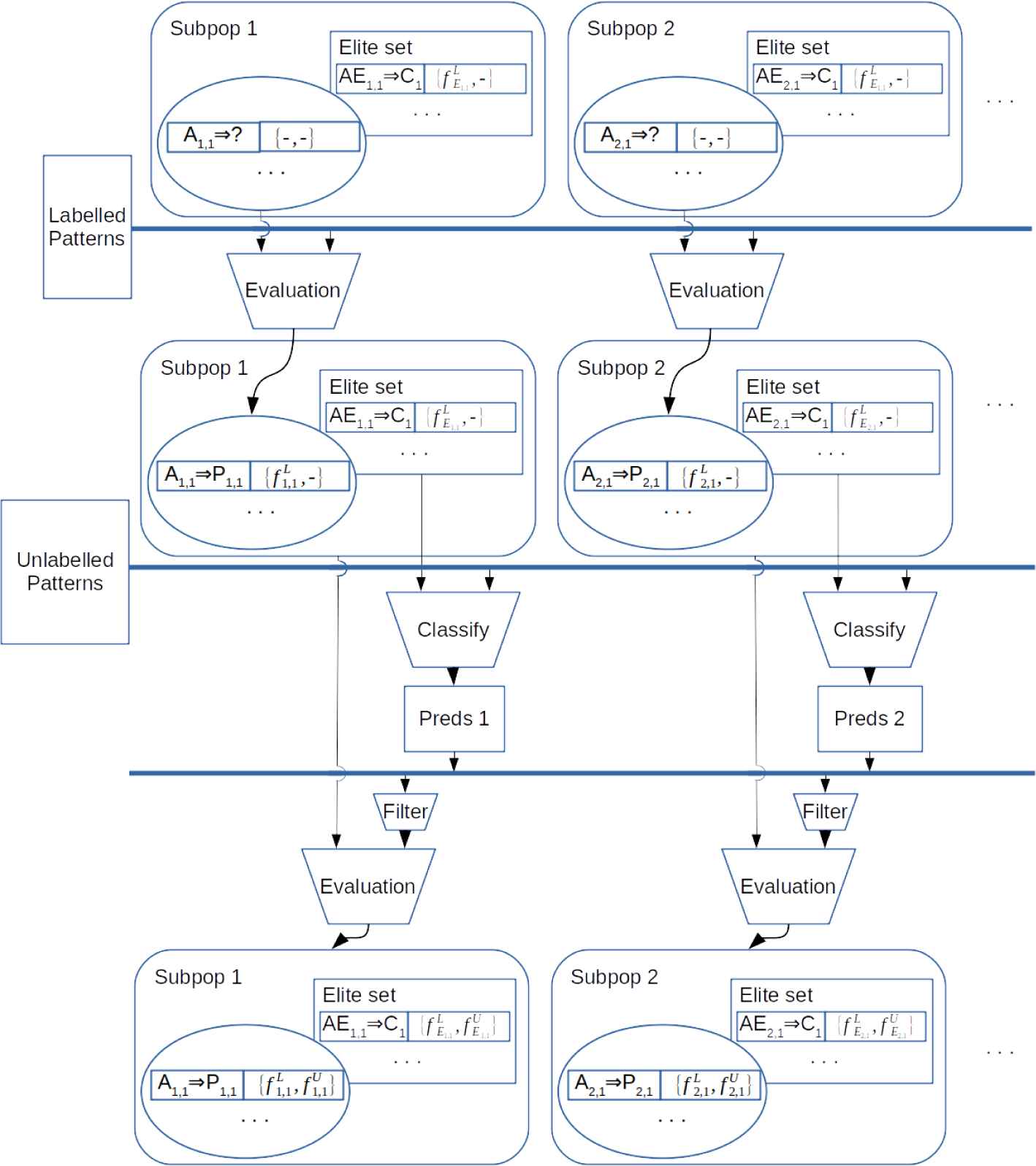
Evaluation phase of our multi-view genetic programming model for semi-supervised rule-based learning. Note that more than two views are possible.
4. EXPERIMENTS
4.1. Experimental Framework
With the intention of extracting conclusions independent of the experiments, as much as possible [40], we have developed an empirical study over a large collection of datasets, up to 25, commonly used in supervised studies. Table 1 summarizes their name, number of patterns, classes and attributes, type of attributes and number of patterns per class. The character “*” in column “Att. Type” indicates that there were some missing values. These datasets have been prepared, through a process referred to as anonymization, to be subject of semi-supervised learning studies in a way similar to that in Ref. [11]. In addition, we have considered four anonymization scenarios. In the first two scenarios, the label of a portion of the patterns of each class is removed. We have removed the label of 95% and 99% random patterns (at least one pattern of each class keeps its label). In the other two scenarios, the label of every pattern is removed except for a specified number
First, the dataset is divided into ten stratified folds (the patterns of each class are shuffled before being assigned to any fold). One of them is used for testing and the rest for training. Every fold will once be used for testing.
Second, the training set is anonymized, i.e., the class label of most of the patterns will be removed to get a large collection of unlabeled samples. As commented before, four anonymization scenarios are considered, 95% and 99% of anonymization, and five and ten nonanonymized samples. Notice that the testing fold is never anonymized.
Third, the classifier is trained with the anonymized training set.
Fourth, the performance of the induced classifier is measured according to the testing fold.
| Id. | Name | #Patterns | #C | #Att | Att. Type |
#Patterns Per Class | |
|---|---|---|---|---|---|---|---|
| Cat | Num | ||||||
| 1 | Australian | 690 | 2 | 14 | 8 | 6 | 383 / 307 |
| 2 | Balance-scale | 625 | 3 | 4 | All numeric | 49 / 288 / 288 | |
| 3 | Breast-cancer | 286 | 2 | 9 | All categoric* | 201 / 85 | |
| 4 | Bupa | 345 | 2 | 6 | All numeric | 145 / 200 | |
| 5 | Car | 1728 | 4 | 6 | All categoric | 1210 / 384 / 69 / 65 | |
| 6 | Chess-KR-KP | 3196 | 2 | 36 | All categoric | 1669 / 1527 | |
| 7 | Cmc | 1473 | 3 | 9 | 7 | 2 | 629 / 333 / 511 |
| 8 | Dermatology | 366 | 6 | 34 | 33* | 1* | 112 / 61 / 72 / 49 / 52 / 20 |
| 9 | Diabetes | 768 | 2 | 8 | All numeric | 500 / 268 | |
| 10 | Digits | 1593 | 10 | 256 | All categoric | Mean 159.3 | |
| 11 | Ecoli | 336 | 8 | 7 | All numeric | 143 / 77 / 52 / 35 / 20 / 5 / 2 / 2 | |
| 12 | Flare | 1389 | 6 | 12 | 2 | 10 | 212/ 287 / 327 / 116 / 51 / 396 |
| 13 | GermanCredit | 1000 | 2 | 20 | 13 | 7 | 700 / 300 |
| 14 | Haberman | 306 | 2 | 3 | 1 | 2 | 225 / 81 |
| 15 | Hypothyroid | 3772 | 4 | 29 | 22* | 7* | 3481 / 194 / 95 / 2 |
| 16 | Ionosphere | 351 | 2 | 34 | All numeric | 126 / 225 | |
| 17 | Iris | 150 | 3 | 4 | All numeric | 50 / 50 / 50 | |
| 18 | Lymph | 148 | 4 | 18 | 16 | 2 | 2 / 81 / 61 / 4 |
| 19 | Page-blocks | 5473 | 5 | 10 | All numeric | 4913 / 329 / 28 / 88 / 115 | |
| 20 | Segment | 2310 | 7 | 19 | All numeric | Each 330 | |
| 21 | Sonar | 208 | 2 | 60 | All numeric | 97 / 111 | |
| 22 | Tae | 151 | 3 | 6 | 2 | 3 | 49 / 50 / 52 |
| 23 | Tic-tac-toe | 958 | 2 | 9 | All categoric | 626 / 332 | |
| 24 | Vehicle | 946 | 4 | 18 | All numeric | 240 / 240 / 240 / 226 | |
| 25 | Zoo | 101 | 7 | 18 | 15 | 2 | 41 / 20 / 5 / 13 / 4 / 8 / 10 |
Datasets considered.

Anonymization process and performance evaluation of the classifier.
To assess the performance of the classifiers, we will first obtain the averaged accuracy and averaged F1 score for each dataset and anonymization scenarios (95%, 99%, five, and ten), i.e., averages are firstly computed over the folds of each dataset and seeds for anonymization (ten folds times five seeds). The accuracy of the classifier
The global performance of the classifiers on the datasets and anonymization scenarios will be aggregated to carry out both parametric analyses, by means of (second) averages, and nonparametric ones, by means of the Friedman ranking methodology [41] (the lower the ranking, the better the algorithm), over the datasets. Note that final averages show the expected results of the methods, where possible global differences may be due to significant deviations on some cases; whereas rankings are invariant to the magnitude of these deviations and emphasize their frequencies. Besides, since rankings are relative, their associated graphs are clearly not monotonous (when one algorithm gets better rankings, the others get worse ones). Without loss of generality, we will present just the analyses that best depict the conclusions we obtained, i.e., those most relevant for the endeavor to induce rule-based classifiers under the multi-view paradigm to our experience, instead of all of those carried out.
Algorithms were implemented in Java 1.8 as an extension of the JCLEC genetic programming module for classification [42–44]. To tune our proposal, most of the combinations of the parameters presented in Table 2 were considered. Notice that only the parameters that directly affect the multi-view methodology were studied by considering more than one value, the rest follow common settings from evolutionary algorithms studies. The best performing parameter setting, which will simply be referred to by MVRB (for Multi-View Rule-Based learning), is boldfaced. The answers to our analyses will be obtained by comparing the results of this best setting with others where just one parameter changes its value. These configurations will be referred to by MVRB(<parameter>=<value>). As a reference point, the results of the WEKA implementation of JRIP [45], which is a fully supervised rule-based classifier inducer and will be trained just on the labeled patterns, is also considered. Besides, although its default parameter settings are used in general, Section 4.6 compares the results of MVRB with those of up to 16 other JRIP configurations.
| Parameter | Values |
|---|---|
| Population size | 100 / |
| 100 among all | |
| the subpopulations | |
| Number of generations | 100 |
| Number of views | 2 / 3 / 4 / 5 |
| Max tree derivation size | 20 |
| Recombination probability | 0.8 |
| Copy probability | 0.1 |
| Mutation probability | 0.2 |
| Consensus-accuracy | linear / |
| combination | increasing linear / |
| lexicographic | |
| Consensus / accuracy ratio | 0.5 / 0.1 / 0.05 / 0 |
| Default class during learning | Yes / No |
| Views convergence | constant / |
| penalization | linearly reduced / |
| no penalization | |
| Max penalization factor | 0 / 0.1 / 0.05 / 0.001 |
Parameter settings.
Our concerns in the following experiments are (1) can the multi-view learning paradigm take advantage from unlabeled patterns to produce better rule-based classifiers? (Section 4.2); (2) how many views should be trained? (Section 4.2); (3) how should the consensus be considered into the evaluation of candidate rules? (Section 4.3); (4) what is the effect of the default classification rule in the learning process? (Section 4.4); (5) what is the effect of imposing a diversified learning process among the views, in an attempt to exploit the complementary principle? (Section 4.5); and finally (6) does our model really produce interpretable rule-based classifiers? (Section 4.6).
4.2. Number of Views
In this first experiment, we are interested on assessing the benefits of using two or more views, up to five, to take advantage from the unlabeled patterns of the training set and produce classifiers better than the one that discards these samples. As mentioned, the quality of the classifier is assessed with regard to the test set, whose patterns are all labeled.
Figure 6 shows the evolution of the averaged accuracy and the aggregated Friedman rankings of the best setting with two, three, four, and five views (MVRB ≡ MVRB(#views=2), MVRB(#views=3), MVRB(#views=4), MVRB(#views=5)), over all the datasets and anonymization scenarios (see Section 4.1), in contrast with that of JRIP and a model that evolves a single population and discards the unlabeled patterns (MVRB(#views=1)). Given that the training of JRIP does not require an evolution process, its performance is presented as a horizontal line for the averaged values (left graphs). Notice that small improvements on several cases cause significant ranking variations. That is why the ranking graphs present many fluctuations. On the other hand, Figure 7 depicts the corresponding evolution of their F1 scores.
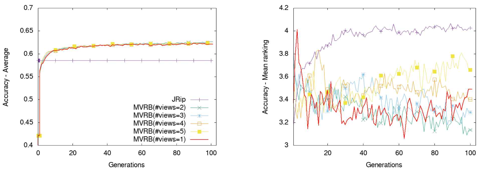
Accuracy of the model with regard to the number of views. Left: averaged accuracy over the datasets and anonymization contexts; Right: mean rankings.

Evolution of the F1 scores. Left: averaged values; Right: mean rankings.
We observe that
The basic ingredients of the genetic programming approach allow our model to obtain better results than those of JRIP, according to both accuracy and F1 score. This means that our base model, a grammar-based genetic programming algorithm, is sufficiently good to match and overcome other alternatives in the literature.
Although all the multi-view algorithms evolve toward better results (graphs on the left), the model with two views obtains slightly better results more frequently than the others (datasets and anonymization scenarios; graphs on the right), although statistical differences were not detected. On the one hand, models with two to four views get better rankings for their F1 scores (Figure 7 right) than models with either one or five views. On the other hand, the model with two views is the one that consistently gets the best rank from the 40th generation on most occasions.
- –
With regard to the model with just one view, this means that the multi-view learning is really taking advantage from the presence of unlabeled patterns to attain better, although slightly, results on more cases.
- –
Regarding the models with more than two views, the presence of many views is introducing some noise into the agreement evaluation (second phase in Figure 4). Then, the confluence to productive levels of agreement needs longer runs to take advantage of the multi-view methodology. To observe this effect, Figure 8 displays the evolution of the ratio of prediction coincidences, on the patterns of the training set, between any pair of views. Although all the models progress toward higher consensus levels, it is clearly noticeable that those with less views advance slightly faster.
- –

Evolution of the ratio of prediction coincidences, on the training set, between any pair of views.
Therefore, we conclude that the multi-view learning methodology is certainly getting benefit from the presence of unlabeled patterns, although slightly with regard to the model with just one view, and that two views seem to perform slightly better than more views, given that in our case, more views introduces noise in the consensus objective.
On the other hand, we shall advise that more computational resources are required as more views are considered in our approach, and our population-based method is more expensive than the heuristic construction of JRIP. In particular according to our implementation, which had not any explicit running optimizations, MVRB(#views=2) consumes up to twice computational time than MVRB(#views=1), and twice time per generation than JRIP, as the average over 100 generations, or 22 times to surpass the accuracy of JRIP (5 generations).
4.3. Consensus Contribution in the Multi-view Learning Process
As commented earlier, the co-training approach, which exploits the consensus principle, aims to minimize the empirical loss on the labeled samples as well as maximizing the agreement among the views on the unlabeled patterns. To do this, most approaches aggregate these two objectives, which becomes the one to be optimized, according to a linear combination such as the one in Eq. (1) for two views.
In our case, every individual of any population has associated two measures,
However, our preliminary experiments showed that the relevance of the consensus part, with regard to the prediction success on labeled patterns, should be much lower. The idea is to avoid that classification errors of some views, more frequent in the first generations of the model, were learned by the other views. Therefore, we have considered up to three different aggregation schemes, whose ranking results on the F1 score metric and prediction agreement are presented in Figure 9. The results of the other metrics are not presented because the accuracy-based rankings were similar to those for the F1 score, and parametric convergence graphs were very similar for all these models. Note that having similar parametric results but different rankings implies that global results are very similar, but small differences appear for many cases in favor of one of the models. MVRB(#consensusCont=linear) applies the mentioned linear combination with
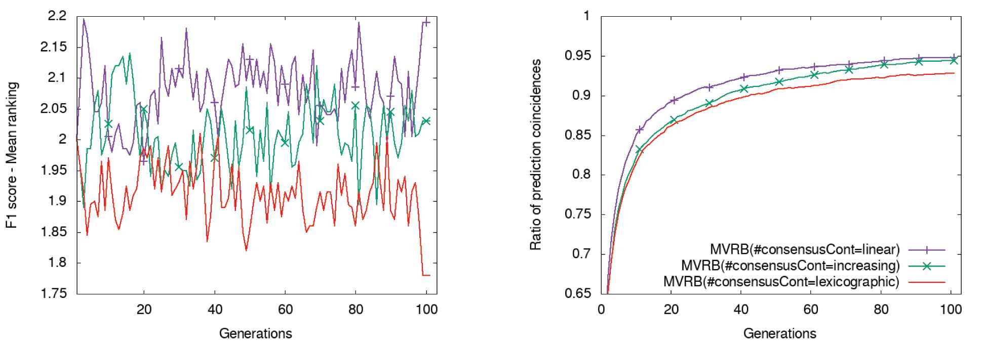
Results of the model with different types of consensus contribution for performance evaluation. Left: evolution of the rankings associated with the F1 score; Right: evolution of the prediction agreement between the two views.
It is very interesting to observe that the model with a lexicographic aggregation consistently obtains the best ranking values from the 40th generation in most occasions, even though its evolution toward higher consensus values is slower. This precisely proves that the linear aggregation is favoring that prediction errors of some views, on unlabeled patterns, are being learnt by the other views at the expense of prediction success on labeled samples. This effect is less evident for the model with increasing consensus relevance in the first generations, given that its
Therefore, we conclude that the lexicographic aggregation provides a more conservative and secure learning process for our model, given that training samples are not wrongly labeled, than the commonly applied linear combination.
4.4. The Default Class Rule in the Learning Process
Rule-based classification systems usually incorporate a default rule to make a decision for patterns not covered by any other rule, otherwise, the classifier would usually not make a prediction for these patterns [36,45,46]. An alternative is to apply a noncrisp rule classification, where the rule whose antecedent's conditions are less violated is selected to make the prediction [47]. However, this scheme is less interpretable than the classic one, because the prediction decision is not so intuitive either when no rule covers the sample or when more than one rule covers it. For this reason, we adopted the classic crisp prediction scheme with an additional default rule.
Given that our preliminary experiments showed that the default rule strongly affected the learning process, we developed experiments with the following two models: MVRB(#defaultRule=yes), where predictions for the second phase of the evaluation step are carried out by the elite sets of the subpopulations with an appended default rule, and MVRB(#defaultRule=no), where the same predictions are carried out by the elite sets without that default class rule. In the first case, the default rule predicts the most frequent class of the training set, among those patterns not covered by any rule of the elite set. In the second case, patterns not covered by any rule are not associated with any prediction and they are discarded for the consensus evaluation. In addition, we also considered a model that do not consider the default rule for the learning process, but it does for the final results on the testing set (the class was selected according to the uncovered patterns of the training set). This last model, MVRB ≡ MVRB(#defaultRule=not_but_in_testing) turned out to be the one with the best results.
Figure 10 presents their ranking evolutions on global accuracy and F1 score. Parametric graphs are not presented because they just showed that MVRB(#defaultRule=no) attained poorer results than the other settings, as these graphs also show. We notice that
In order to get good results, the final solution must incorporate a default rule, because the model that do not use it obtains the worst, higher, rankings.
The model that does not apply the default rule during the learning process, but it does for testing, provides better accuracy and F1 scores than the one that uses it all the time. This implies that the default rule is introducing noise in the learning process. In particular, all the patterns not covered by any rule and wrongly predicted by the default rule, in any view, are misleading the other views. Therefore, it is better to promote the consensus between the views just on the covered patterns, which are those where the predictions of the views are more reliable.
Comparing the extreme cases, the model that never considers the default rule and the one that always uses it, it is interesting that their F1 scores are closer than their accuracy results. This is showing that the default rule is particularly harmful on imbalanced datasets, because the default rule causes poor results for little represented classes.

Results of the model with and without the intervention of a default class rule in the learning process. Left: evolution of the rankings associated with the averaged accuracy over the datasets and anonymization contexts; Right: evolution of the mean rankings for the F1 scores.
Then, we conclude that predictions, used to evaluate the agreement among the views, should not be obtained from classifiers that include default rules; however, their usage is necessary for the final classifier.
4.5. Imposing Diversification Among the Views
The complementary principle, together with the consensus one, is said to be responsible for multi-view learning to attain good results. It states that each view of the data should contain some knowledge that other views do not have [4]. Aiming at taking some benefits from this principle, we examined whether promoting some divergence among the classifiers might be advantageous. Our idea was to promote that populations use different attribute sets, so we introduced a penalization factor that reduced the fitness of the individuals according to the appearance frequency of the used attributes in the other views. Eq. (9) regulates this penalization, where
For models MVRB(#penalization=yes), which always applies Eq. (9) with
Imposing a diversified search among the views is not producing as good results as allowing the views to converge from the initial generations (Figure 11 left). Between the two models that impose diversification, the one that decreases the penalization is able to get just slightly better results.
Imposing diversification is clearly hindering the views to reach consensus on the predictions for the patterns. Besides, although the model with a decreasing penalization attains more prediction agreements than the model with constant penalization, it advances very slowly and finishes with consensus results far lower than the model that does not apply penalization at any step.

Results of the model with and without penalization for using frequent pattern attributes. Left: evolution of the averaged accuracy; Right: evolution of the consensus among the views.
The conclusion of this experiment is that imposing a diverse search among the different views, in an attempt to get some benefits from the complementary principle, is not reporting the expected good results, at least according to the way we promoted that diversification.
4.6. Interpretability
Comprehensibility is one of the benefits that rule-based systems possess and have attracted the attention of researchers [17–19,21,48]. One of the most common ways to evaluate the interpretability of rule-based systems is counting the number of conditions present in their rules. Less conditions, more comprehensibility. Figure 12 shows the evolution of the number of conditions in the rule-based classifiers induced by MVRB, with regard to those of JRIP.

Evolution of the number of conditions of the rule-based classifiers.
We observe that our model consistently produces simple rule systems with an average of five conditions along the generations, but JRIP produces classifiers with even less conditions, so more interpretable. However these simpler rule systems had worse performances (see Figures 6 and 7).
It is particularly interesting to observe that the averaged number of conditions in the classifiers of JRIP is quite less than the averaged number of classes in the considered datasets (3.88, see Table 1). This implies that JRIP is producing classifiers with default rules, which do not have any condition in the antecedent, and thus, classifiers without rules for some of the classes. In order to analyze whether this fact is causing its inferior performance, we compare JRIP with different parameter settings, which are expected to directly affect the rules in the generated classifiers, against MVRB. These parameters are, according to the documentation2 and in this order, the number of runs of optimizations (default is 2), whether to use or not to use pruning (default is true), and whether to check or not to check if the error rate is greater than or equal to 0.5 in its stopping criteria (default is true; therefore, previous runs of JRIP are those of JRIP(2,true,true)).
Table 3 shows the p-values of the Wilcoxon paired signed-rank test when comparing the results, in accuracy and F1 score, of both algorithms per anonymization context, together with the average of conditions in their classifiers. The null hypothesis is that the median difference between pairs of observations is zero. The classifiers from the last generation of MVRB are used. The sign preceding each p-value indicates whether the sum of the Wilcoxon rankings of the first method, in this case JRIP, is greater than the sum of the rankings of the second one, that of MVRB (
| Anonym. |
95% anonym. |
99% anonym. |
5 non-anonym. |
10 non-anonym. |
Wins |
Losses |
||||||||||
|---|---|---|---|---|---|---|---|---|---|---|---|---|---|---|---|---|
| JRIP vs. MVRB | Acc. | F1 | C | Acc. | F1 | C | Acc. | F1 | C | Acc. | F1 | C | Acc. | F1 | Acc. | F1 |
| JRip(0,false,false) | 4.1 | 8.8 | 8.9 | 1.7 | 2 | 3 | 0 | 0 | ||||||||
| JRip(0,false,true) | 5.3 | 9.6 | 9.4 | 2.2 | 1 | 2 | 0 | 0 | ||||||||
| JRip(0,true,false) | 2.3 | 4.5 | 4.4 | 0.7 | 3 | 4 | 0 | 0 | ||||||||
| JRip(0,true,true) | 3.0 | 4.9 | 4.2 | 0.9 | 2 | 4 | 0 | 0 | ||||||||
| JRip(1,false,false) | 4.1 | 8.8 | 8.9 | 1.7 | 2 | 3 | 0 | 0 | ||||||||
| JRip(1,false,true) | 5.3 | 9.6 | 9.4 | 2.2 | 1 | 2 | 0 | 0 | ||||||||
| JRip(1,true,false) | 2.7 | 4.2 | 3.4 | 0.6 | 2 | 4 | 0 | 0 | ||||||||
| JRip(1,true,true) | 2.6 | 4.0 | 3.4 | 0.6 | 2 | 4 | 0 | 0 | ||||||||
| JRip(2,false,false) | 4.1 | 8.8 | 8.9 | 1.7 | 2 | 3 | 0 | 0 | ||||||||
| JRip(2,false,true) | 5.3 | 9.6 | 9.4 | 2.2 | 1 | 2 | 0 | 0 | ||||||||
| JRip(2,true,false) | 2.9 | 4.3 | 3.6 | 0.7 | 1 | 4 | 0 | 0 | ||||||||
| JRIP |
2.8 | 4.2 | 3.6 | 0.7 | 1 | 4 | 0 | 0 | ||||||||
| JRip(4,false,false) | 4.1 | 8.8 | 8.9 | 1.7 | 2 | 3 | 0 | 0 | ||||||||
| JRip(4,false,true) | 5.3 | 9.6 | 9.4 | 2.2 | 1 | 2 | 0 | 0 | ||||||||
| JRip(4,true,false) | 3.1 | 4.5 | 3.9 | 0.7 | 1 | 2 | 0 | 0 | ||||||||
| JRip(4,true,true) | 3.0 | 4.5 | 3.9 | 0.7 | 1 | 2 | 0 | 0 | ||||||||
| MVRB | 4.7 | 4.3 | 4.2 | 4.1 | ||||||||||||
p-Values of the Wilcoxon paired signed-rank test on accuracy and F1 score per anonymization scenario, between each JRIP setting and MVRB, and the number of conditions of their classifiers.
As can be seen, although the comparison favors different JRIP settings (
5. CONCLUSIONS
We have presented a model for obtaining interpretable rule-based classifiers for semi-supervised contexts, which follows the multi-view co-training methodology on single-source data. To our knowledge, this is the first study involving multi-view learning and rule-based classifiers. The model is a grammar-based genetic programming algorithm that evolves multiple views and promotes the generation of classification rules that both accurately predict the class of labeled patterns and agree with the predictions of the other views for unlabeled examples.
Our study details the peculiarities that multi-view learning with rule-based classifiers brings about, since common practices may not produce the expected results. In particular, we have observed that
The multi-view learning approach may really allow the learning process to take advantage of the presence of unlabeled patterns to induce, although slightly, better classifiers.
Too many views slows down the convergence towards good classifiers, because noise is introduced into the consensus objective. In our case, two views were enough.
Our model with a lexicographic aggregation scheme attained better performance scores than the commonly applied linear combination between the accuracy on labeled patterns and the agreement among the views for unlabeled ones. This occurred because the linear combination was favoring wrong predictions of some views to be learnt by other views.
The use of default rules, when obtaining the predictions for evaluating the agreement among the views, is discouraged, given that they are unreliable and will probably mislead other views. On the other hand, they are required to get good final results (in the testing and deployment stages).
Favoring that views evolve with different attribute sets, in an attempt to exploit the complementary principle in single-source cases, probably makes difficult to get a good single classifier.
We think that this line of research is worthy of further studies, particularly given that the combination of multi-view learning and rule-based classifiers has not been very much studied. We intend to explore the following avenues: (1) to consider other diversity measures and application schemes that might favor the exploitation of the complementary principle; (2) to search for rule-based classifiers under the multi-view methodology and other search models apart from genetic programming, such as iterated greedy [21]; and (3) to analyze whether better rule-based classifiers can be obtained under the multi-view paradigm where other views make use of other and more powerful base classifiers, such as neural networks.
CONFLICT OF INTEREST
Carlos García-Martínez and Sebastián Ventura, authors of the work with title “Multi-view genetic programming learning to obtain interpretable rule-based classifiers for semi-supervised contexts. Lessons learnt.” have no competing interests to declare.
AUTHORS' CONTRIBUTIONS
All authors, Carlos García-Martínez and Sebastián Ventura, contributed equally to this work, in the literature search, study design, computational experimentation, data analysis, and manuscript writing.
ACKNOWLEDGMENTS
This research is supported by the project of the Spanish Ministry of Science and Technology TIN2014-55252-P, TIN201783445P and FEDER funds.
Footnotes
This work is a major extension of our initial study [27]. Much more datasets and anonymization contexts are considered here, and other algorithmic aspects are analyzed. Concretely, more detailed descriptions of the method and experimentation are provided, Sections 4.3, 4.4, and 4.5 are completely new, and just Figures 1–4 appeared there (four out of 12).
REFERENCES
Cite this article
TY  - JOUR
AU  - Carlos García-Martínez
AU  - Sebastián Ventura
PY  - 2020
DA  - 2020/05/25
TI  - Multi-view Genetic Programming Learning to Obtain Interpretable Rule-Based Classifiers for Semi-supervised Contexts. Lessons Learnt
JO  - International Journal of Computational Intelligence Systems
SP  - 576
EP  - 590
VL  - 13
IS  - 1
SN  - 1875-6883
UR  - https://doi.org/10.2991/ijcis.d.200511.002
DO  - 10.2991/ijcis.d.200511.002
ID  - García-Martínez2020
ER  -