
A Novel Density Peaks Clustering Algorithm Based on Local Reachability Density
- DOI
- 10.2991/ijcis.d.200603.001How to use a DOI?
- Keywords
- Clustering algorithm; Density peaks clustering; Local reachability density; Domino effect
- Abstract
A novel clustering algorithm named local reachability density peaks clustering (LRDPC) which uses local reachability density to improve the performance of the density peaks clustering algorithm (DPC) is proposed in this paper. This algorithm enhances robustness by removing the cutoff distance dc which is a sensitive parameter from the DPC. In addition, a new allocation strategy is developed to eliminate the domino effect, which often occurs in DPC. The experimental results confirm that this algorithm is feasible and effective.
- Copyright
- © 2020 The Authors. Published by Atlantis Press SARL.
- Open Access
- This is an open access article distributed under the CC BY-NC 4.0 license (http://creativecommons.org/licenses/by-nc/4.0/).
1. INTRODUCTION
Clustering analysis, a type of unsupervised classification, is a primitive exploration of data with little or no prior knowledge, a kind of data mining technique to seek features of unlabeled data and assigns a new input to one of a finite number of discrete unsupervised categories according to their similarity [1]. Several methods of clustering analysis have been proposed, including the hierarchical, partitioning, density-based, model-based, grid-based, and graph theory methods [2], although they use different notions for similarity. All these methods follow the same principle that patterns of data in a cluster should be similar, while patterns of data in different clusters should be different [3]. Nonpredictive clustering is a subjective process in nature, precluding an absolute judgment with regard to the relative efficacy of all clustering techniques [4,5].
In 2014, Rodriguez et al. proposed a density-based clustering algorithm called “density peaks clustering” (DPC) [6]. The core of this algorithm is the observation of the decision graph, which is generated by using local density ρ and its distance δ. The DPC has capacity to determine clustering centers automatically and deal with arbitrary-shaped clusters, depending only on the distance between data points, as well as a user-defined parameter dc. Once the cluster centers are identified, each of the remaining points is assigned to a cluster which is the same cluster as its nearest higher density neighbor belongs to. This leads to two deficiencies: (i) the assignment process is likely to trigger a domino effect [7] and (ii) the value of cutoff distance is crucial to an assignment, but the fault tolerance of its calculation is poor.
Several research projects have been carried out to improve the capabilities of the DPC. Jiang applied the DPC based on k nearest neighbors to deal with the domino effect [8]. Chen estimated ages using the DPC and the distances of facial image to peaks [9]. The principal component analysis was applied by Du to enable the DPC to handle high-dimensional data more effectively [10]. An improved DPC method was utilized to discover social circles with overlap on account of user’s profile and topological features [11]. By far, the aforementioned defects of the DPC were not addressed sufficiently.
In order to overcome the problems in the DPC, a new clustering algorithm is proposed in this paper, in which the local density in the DPC is replaced with the local reachability density or lrd, in conjunction with a novel assignment strategy, which is developed to enhance the robustness and tackle the domino effect that often occurs with the DPC.
The rest of the paper is set out as follows: In Section 2, the principle of the DPC is introduced and the concept of local reachability density is defined. Section 3 details the method proposed in this paper and illustrates the algorithm procedures. The experimental results are presented in Section 4 to verify the feasibility and efficiency of the proposed algorithm, and finally the conclusions are drawn in Section 5.
2. THEORETICAL BACKGROUND
2.1. Density Peaks Clustering Algorithm
In the DPC, it is assumed that a cluster center has higher local density than its neighbors and the cluster center point has relatively larger distances from other points of higher density. There are two ways to calculate local density ρ. The one is using the cutoff kernel, i.e., the number of data points in the neighborhood of a cluster, which is defined as
The other way is using the Gaussian kernel [12], as following:
The Gaussian kernel can be seen as a smoothed cutoff kernel. For both Eqs. (1) and (2), as a rule of thumb, dc has been chosen so that the average number of neighbors is between 1% and 2% of the total points in a dataset.
Let δi be the minimum distance from point i to any other points in a data neighborhood, i.e.,
2.2. Local Reachability Density
Since the distribution of data objects varies from one local spatial region to another, it is impossible to examine each data object with a globally unified standard. Specialized parameter that suits individual data object is desirable. Investigations for achieving individual parameter were reported in 2000 by Breunig et al. A density-based local outlier identification algorithm was proposed in which a novel form of density called the local reachability density (lrd) was introduced [13]. In order to calculate lrd, the concept of k-distance, k-distance neighborhood and reachability distance are defined as follows:
Definition 1.
(k-distance of an object p)
For any positive integer k, the k-distance of object p, denoted as k-distance(p), is defined as
for at least k objects
for at most
Based on this definition, the range of an individual local spatial area for a data object is determined by examining the distance between each data object and the other data objects under investigation, therefore the k-th distance from the maximum to the minimum can be found. In areas with high object density are featured with shorter k-distance in general; on the contrary, areas with low data object density correspond to larger value of k-distance.
Definition 2.
(k-distance neighborhood of an object p)
Given the k-distance of data object p, the k-distance neighborhood of p contains every object whose distance from p is no greater than its k-distance, and hence the number of data objects contained in the neighborhood, N(p) can be found from the following equation:
N(p) is the number of collected data objects in a neighborhood which is centered by an object under investigation with the k-distance as the radius. For data objects with a higher degree of deviation, the area covered by the set is larger; while for data objects with lower deviation, the set covers a smaller area. For the data objects in the same cluster group, their k-distances cover roughly the same area.
Definition 3.
(reachability distance of object p with respect to object o)
Let k be a natural number. The reachability distance of object p with respect to object o is defined as
This definition means the larger one between k-distance at point o and distance between point p and o is chosen as the reachability distance of p with regard to object o.
Definition 4.
(local reachability density of an object p)
The local reachability density of p is defined as
In essence, if a given data object p is in a certain cluster group, the probability of p in the k-distance of neighborhood o is high, where o is in the k-distance of neighborhood p. Therefore, the probability that the
3. LOCAL REACHABILITY DENSITY PEAKS CLUSTERING
In this paper, a novel algorithm that uses the local reachability density peaks clustering (LRDPC) is proposed to compensate the deficiencies of the DPC. In the LRDPC, the sensitive parameter dc is removed from calculation, and the domino effect generated by the DPC allocation strategy is avoided.
In the DPC, a local density ρi is equal to the number of points enclosed by the radius of dc with regard to point i, whilst in the LRDPC, the local reachability density lrd(i) is the inverse of average reachability distance based on the number of neighbors around point i. Different from local density ρi, lrd(i) uses the concept of k-distance neighborhood to define the local reachability density. In the LRDPC, the distance is defined as follows:
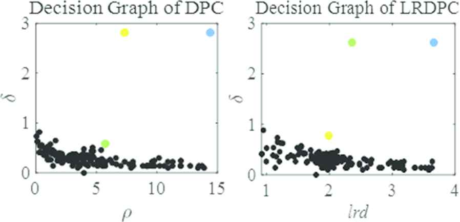
Using lrd as the abscissa and δ as the ordinate, the decision graph can be generated. Cluster centers are those that have both relatively large lrd and extremely large δ. As shown in Figure 1, in this example, the three cluster centers are obviously recognizable as they are all in the upper right area of the decision graph.
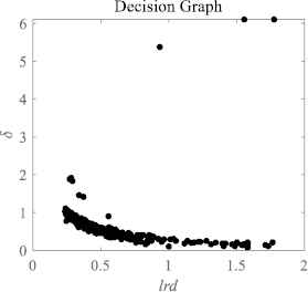
Decision graph of Spiral dataset.
After the total of n cluster centers are selected, a unique set of data points are contained by each cluster, each set being represented as Cj, j = 1, 2 … n. Except the clustering centers, all other points in each set are sorted in a descending order of lrd, along with their k-distance neighborhoods. For each center point i, the number of data points, N(i) in a given cluster based on its k-distance neighborhood can be found. The weight, lrd-weight(i, j) of a given data point i, in Cj is defined as
For a given data point i, Eq. (5) is applied to identify each cluster and its correspondent N(i) number of k-distance neighborhood, and then the sum of lrd in each Cj is calculated separately.
Eq. (6) is used to find the maximum lrd-weight(i, j) and then point i is assigned to the cluster set Cj. The assignment aggregation process is defined as
The procedures of the algorithm LRDPC, governed by Eqs. (4–6) are outlined as follows:
4. EXPERIMENTS
4.1. Performance on Datasets
The performance of the LRDPC algorithm has been evaluated using the standard datasets such as the Spiral [15], Pathbased [15], Aggregation [16], R15 [17] and Db-moon, as well as real-world datasets, Iris [18] and Wine [19]. In order to demonstrate the superiority of this algorithm, some classical clustering algorithms, including the DBSCAN [20], the K-means [21] and the DPC are also tested on these datasets. The foregoing datasets along with their properties are provided in Table 1.
| Datasets | Objects | Features | Clusters |
|---|---|---|---|
| Spiral | 312 | 2 | 3 |
| Aggregation | 788 | 2 | 7 |
| Pathbased | 300 | 2 | 3 |
| R15 | 600 | 2 | 15 |
| Db-moon | 400 | 2 | 2 |
| Iris | 150 | 4 | 3 |
| Wine | 178 | 13 | 3 |
Standard datasets features.
The F-Measure, which is used to assess the accuracy of an algorithm, is widely utilized in statistical analysis [22]. In this paper, this measure is employed to evaluate the performance of each algorithm in Table 1.
The F-Measure is a weighted harmonic mean of precision and recall, where precision P is obtained from the number of correct positive results divided by the number of all positive results returned by the classifier, while recall R is the number of correct positive results divided by the number of all relevant samples. When the weight of precision and recall is equal, the F-Measure becomes F1-Measure, where the score reaches its best value at 1 corresponding to the perfect precision and recall, and it reaches the worst at 0. Some parameters are closely related to precision and recall are introduced in Table 2.
| Relevant | Nonrelevant | |
|---|---|---|
| Retrieved | True positives (TP) | False positives (FP) |
| Not retrieved | False negatives (FN) | True negatives (TN) |
Parameters related with F1-Measure.
Algorithm in this work: LRDPC
Require: Distance matrix D∈RNxM, k
Step 1: Calculate lrd
1.1 Calculate k-distance based on
1.2 Calculate k-distance neighborhood based on Definition 2;
1.3 Calculate reachability distance based on Definition 3;
1.4 Calculate local reachability density based on Definition 4.
Step 2: Identify cluster centers by decision graph
2.1 Sort lrd in a descending order;
2.2 Calculate δ based on Eq. (4);
2.3 Generate the decision graph;
2.4 Select an area in decision graph to identify cluster centers;
2.5 Create a set for each cluster center, and record it as Cj,
Step 3: Assign each point to different clusters
3.1 Calculate lrd-weight based on Eq. (5);
3.2 The remaining points in set U are taken out in descending order and added to the set Cj of the largest lrd-weight based on Eq. (6). Judge whether it meets the criteria: U is an empty set. If satisfied, output Cj,
In Table 2, Precision P and recall R are defined as follows:
The performance of binary tasks is not the only consideration, and improvements in examination of precision and recall are required too. These two issues are addressed by the following straightforward approach. The precision and recall rates on each confusion matrix are calculated from which their mean values are determined. Taking the effects of P and R equivalently into account, the macro F1-Measure is defined as
In the experiments, all the parameters were set to optimal. For examples, for the DBSCAN, the parameters ε and MinPts were adjusted until the classifier was at its best performance; when applying the K-means, the number of clusters K was set to a number which was the same as the correct number of clusters; the cutoff distance dc for the DPC was set to such a value that the average number of neighbors was equal to 2% of the total number of points in the dataset; and the positive integer k for the LRDPC was chosen from 6 to 9. In order to take each feature into equal consideration, all nongeometric features were normalized. The performances of different algorithms are compared based on their application results for each data type using the figures and tables below.
The first dataset used for tests was a two-dimensional (2D) dataset, known as the Spiral. The Spiral contains 312 objects, which are divided into three clusters, and each featured with a spiral line. Credited with its ability in discovery of clusters with arbitrary shapes [5], the DPSCAN algorithm performed very well on this dataset. As shown in the upper right graphs in Figure 2, all data points were correctly clustered. In contrast, the algorithm K-means was confused, resulting in the clusters with mixed up data objects. When the K-means applied, the data in each new cluster became orderless, and many original data points were incorrectly grouped. This is because the K-mean has a difficulty to converge for nonconvex datasets [23]. The results with K-means are depicted with the upper left graphs in Figure 2. Both the DPC and LRDPC worked effectively on this dataset as depicted in Figure 2.
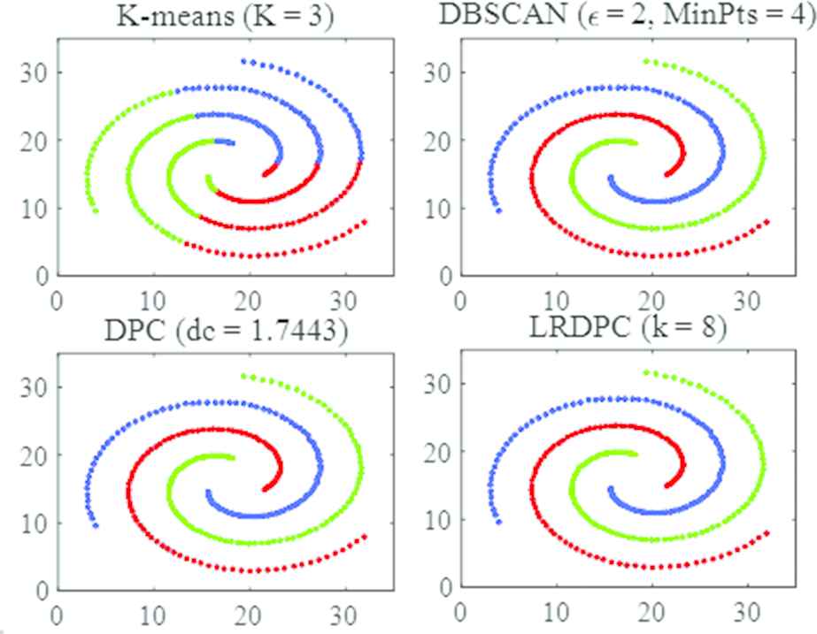
Aggregation of the Spiral dataset using different algorithms.
The Pathbased is another standard dataset with 300 objects which are contained in three clusters. The three clusters include a gapped ring cluster and two others that are enclosed by this ring. The DBSCAN algorithm had the worst performance with the lowest F1-measure value on this dataset, and even the number of clusters was incorrectly identified. The clustering results with the LRDPC were similar to that with the DPC and K-means. Although none of them was perfect, the LRDPC achieved the best F1-measure value. The detailed F1-measure comparison can be seen in Table 3. The clustering results of the four algorithms on the dataset Pathbased are shown in Figure 3.
| Datasets | K-means | DBSCAN | DPC | LRDPC |
|---|---|---|---|---|
| Spiral | 0.3268 | 1 | 1 | 1 |
| Aggregation | 0.4248 | 0.9003 | 1 | 1 |
| Pathbased | 0.7082 | 0.1830 | 0.6936 | 0.7176 |
| R15 | 0.8831 | 0.6406 | 1 | 1 |
| Db-moon | 0.7897 | 1 | 0.8304 | 1 |
| Iris | 0.8918 | 0.4338 | 0.8240 | 0.9048 |
| Wine | 0.9512 | 0.2100 | 0.5287 | 0.9341 |
LRDPC, local reachability density peaks clustering; DPC, density peaks clustering.
F1-Measure of algorithms on datasets.
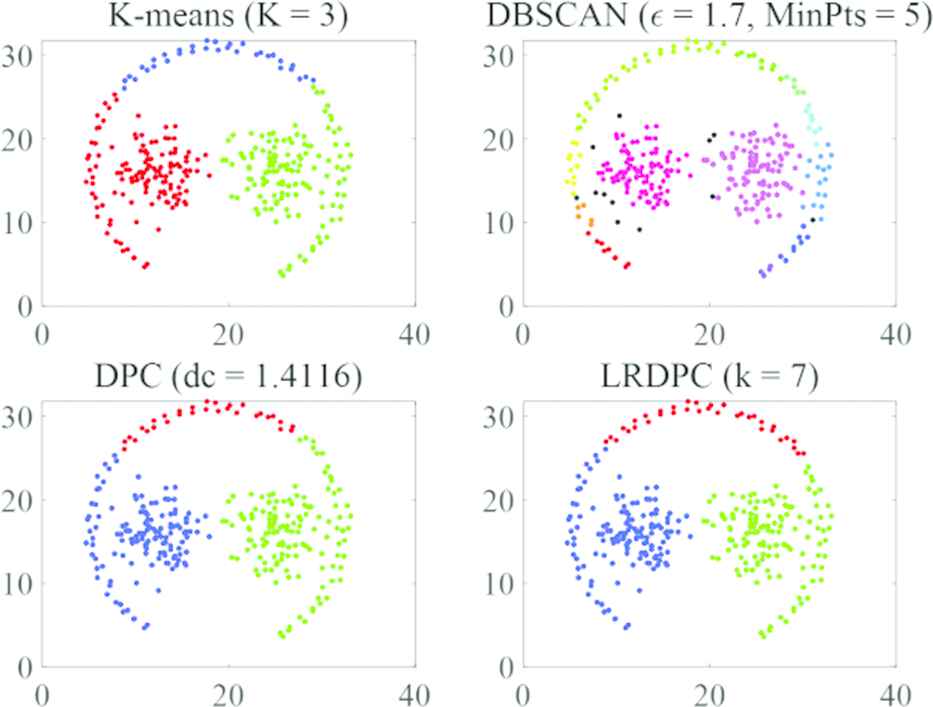
Aggregation of the Pathbased dataset using different algorithms.
Both the DPC and LRDPC allocated all data points correctly and have the best performance on the datasets R15 and Aggregation. In the tests, the number of cluster centers were obtained correctly from their decision graphs, and all the points were divided into the correct clusters. The results are shown in Figures 4 and 5.
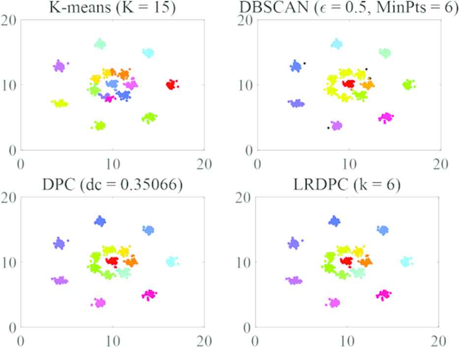
Aggregation of the R15 dataset using different algorithms.
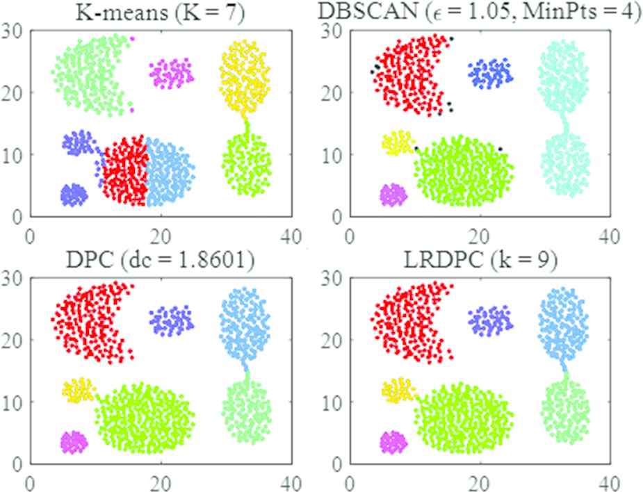
Aggregation of the Aggregation dataset using different algorithms.
As shown in Figure 6, the Db-moon is a synthetic dataset composed of two similar crescent clusters, with a total of 400 2D. The DBSCAN worked perfectly, and every point was assigned into the correct cluster by carefully selecting the hyper-parameters. The same results were obtained by applying the LRDPC, and it must be noted that the LRDPC outperformed the DPC on this dataset. In the case of applying the DPC, a single point was misallocated in the clustering process, which triggered the domino effect, resulting in almost half of a cluster data points being incorrectly grouped. The details can be seen in Figure 6.
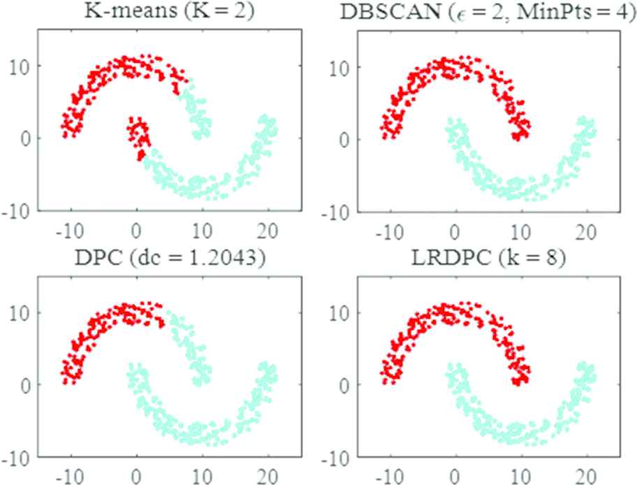
Aggregation of the Db-moon dataset using different algorithms.
The results on the performance of the DBSCAN, K-means, DPC and LRDPC measured by F1-Measure are given in Table 3. The bold numbers are used to indicate that the algorithm performed best on a given data set. It can be seen from Table 3 that K-means has no ability to deal with nonconvex datasets due to its iterative approach. The robustness of the DPC is poor, and it performed poorly on the four datasets. In addition, if the clustering is not entirely correct, more errors can occur due to the domino effect for the DPC, which was demonstrated when dealing with the Db-moon data set. Among these algorithms, the LRDPC achieved the highest F1-score on almost every dataset, and even on the Wine, very good results were obtained, showing its broad adaptability and robustness.
4.2. Superiority of Local Reachability Density
Instead of local density ρ and distance δ, the local reachability density lrd is used to generate decision graph in the LRDPC. The geometric meaning of lrd is the inverse of the average reachability distance, which implies that it takes the characteristics of each cluster into consideration, rather than treating the entire dataset as a whole. Doing so gives rise to two advantages: one is that the cluster centers can be identified more accurately based on a decision graph, and the other is that more reasonable density-based sorting can be ensured. The advantages of the LRDPC were further tested on the real-world datasets, the Iris and the Wine.
The Iris is a real-world dataset with four dimensions, which is divided into three clusters. In the tests, the LRDPC achieved the highest F1-score, considerably higher than that by the DPC on this dataset which can be seen in Table 3. Figure 7 are the decision graphs generated by using both algorithms. The graph on the right-hand side, generated by the LRDPC, has three outliers. However, the left-hand side decision graph, generated by DPC, can hardly get three cluster centers, let alone aggregate data accurately.
Decision graphs of density peaks clusteringDPC and local reachability density peaks clustering (LRDPC) on dataset Iris.
The Wine is a high-dimensional dataset from the real-world, on which, the LRDPC significantly outperformed the DPC and other algorithms, just slightly fell behind the K-means.
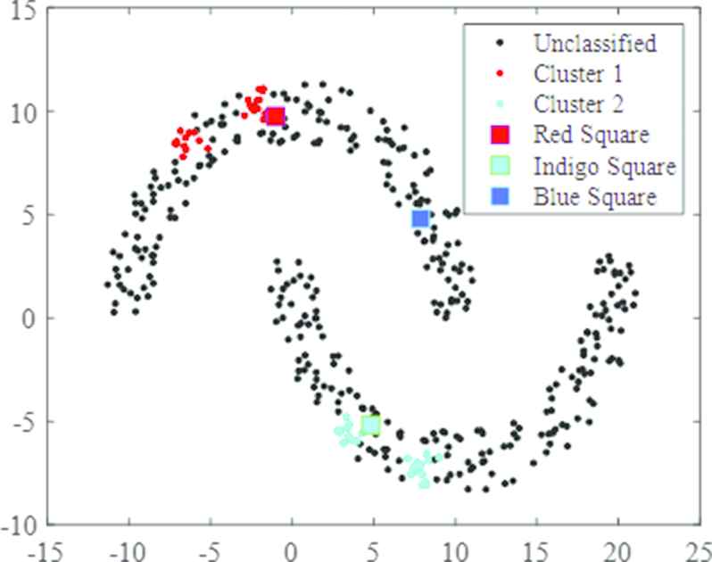
Figures 8 and 9 depict clustering processes of the DPC and LRDPC on dataset of Db-moon. The red and indigo dots indicate those data that have already been aggregated and the blue square represents a point waiting for clustering. Figure 8 shows how a cluster is identified to contain the blue square using local density as a sort benchmark. The red square is the nearest point to the blue square in cluster 1, while the indigo square is the nearest data point to the blue square in cluster 2. The distances between the blue square to red and indigo squares are 13.9991 and 7.6395 respectively, which means the blue square should be aggregated to cluster 2. However, it is obvious, this blue square should be in Cluster 1. This example demonstrates that using local density as sort benchmark as in the DPC can trigger an incorrect clustering process, which has serious detrimental effect. Figure 9 shows the method LRDPC is used to determine the cluster for the same blue square using the reachability density lrd as a sort benchmark. It can be seen that in this case although the original two squares are still the nearest to the blue square, the sequence in distance has been changed. Now between the red and blue squares, the distance is 3.4703 and between the indigo and blue it is 16.6912. As a result, the blue square is clustered into Cluster 1 correctly.
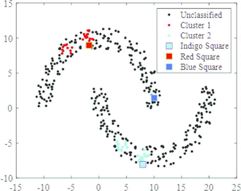
Clustering process of density peaks clustering (DPC) on dataset Db-moon.
Clustering process of local reachability density peaks clustering (LRDPC) on dataset of Db-moon.
4.3. Domino Effect in DPC
According to sample assignment strategy of the DPC, the nearest neighbor of an incorrectly allocated sample is likely to be aggregated to the same cluster as a result. This is because the allocation of the point is based only on its nearest neighbor’s cluster information. This error distribution effect hidden by the allocation strategy is proven fatal, which can cause a series of errors once a sample is assigned incorrectly. This is known as the “domino effect” in aggregation.
Figure 10 is a partially zoomed view of the Spiral data set sorted using the DPC with dc equals to 0.9394, making the average number of neighborhood equal to 1% of the total number of objects in the dataset. The area defined by abscissa from 2 to 12 and the ordinate from 10 to 30 is intercepted from the original dataset. All the samples are sorted in a descending order of the local density ρ, and the serial numbers are marked on the graph. The red dot labeled 251 is the 251th assigned point. The point closest to it on its spiral line that has larger local density ρ is the blue dot labeled 239. The distance between them is 4.2202. However, the point where the local density is greater than point 251 and closest to it is the red dot labeled 168, with a distance 4.1743. Since point 251 is closer to point 168 than to point 239, it is assigned to the same cluster that contains point 168. As point 251 is misallocated, consequently point 253 is also incorrectly assigned. This triggers the domino effect, all points after point 251 in cluster 3 are subsequently misallocated to Cluster 1.
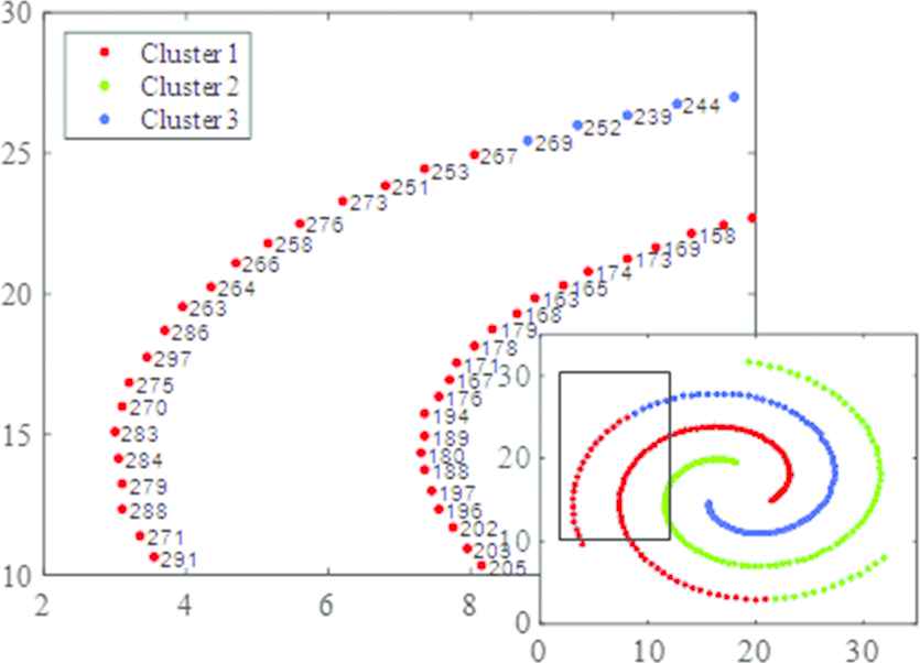
Partial enlarged view of Spiral using density peaks clustering (DPC) with dc equals to 0.9394.
Figure 11 is a partially enlarged view of the Spiral data set, intercepting the same area as defined in Figure 10. However, the data are sorted using the LRDPC with k of 7. The point 251 in Figure 10 is marked as point 259 in Figure 11, which is artificially classified. The point to be assigned next is point 260, and its k-distance neighborhood contains the square-framed points 264, 261, 259, 258, 256 and 253. Among them, points 264 and 261 are points that have not been assigned yet. The lrd-weights of the three clusters calculated based on Eq. (5) are 0.3820, 0 and 1.1576 respectively. According to the proposed allocation strategy, point 260 should be assigned to the correct cluster. In contrast to the DPC, the domino effect does not occur.
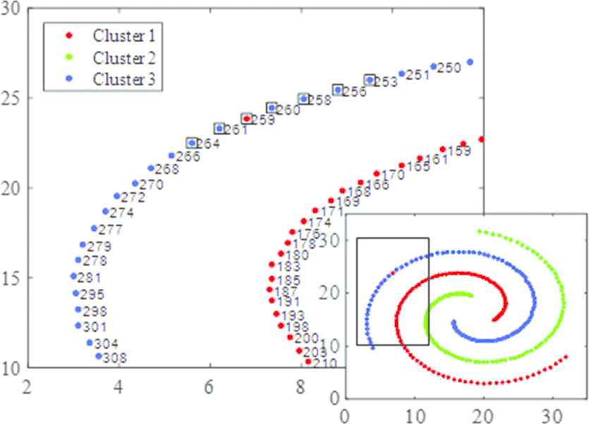
Partial enlarged view of Spiral using local reachability density peaks clustering (LRDPC) with k equals to 7.
4.4. Sensitivity Analyses
The cutoff distance dc in DPC is important to the assignment while has poor fault tolerance. DPC claims that one can choose dc so that the average number of neighbors is around 1% to 2% of the total number of points in the data set. To study the sensitivity of DPC, dc was set to 0.618, 0.939, 1.367, 1.744 respectively, makes the average number of neighbors of the total number of points in the data set equals to 0.5, 1, 1.5, 2%, respectively. The performance on the dataset Spiral is shown in Figure 12. It can be seen that except when
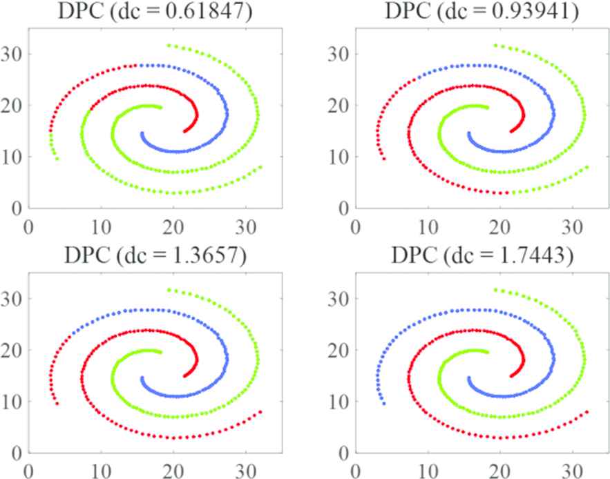
Sensitivity analyses of density peaks clustering (DPC).
As a contrast, the parameter k in LRDPC was set to 6, 7, 8 and 9 respectively, and the performance is also verified on the dataset Spiral. The results are shown in Figure 13. It can be seen that LRDPC is insensitive to its parameter k and has stronger robustness. According to the experimental experience, the value of k is recommended as the positive integer from 5 to 10.

Sensitivity analyses of local reachability density peaks clustering (LRDPC).
5. CONCLUSION
Based on the analysis of the experimental results, it can be concluded that the LRDPC has several advantages over the DPC: (i) On the standard datasets, the overall result of F1-measure of the LRDPC is better than the DPC. The LRDPC also performs better than other algorithms on the real-world dataset. (ii) From the geometric meaning, use of lrd is more suitable for clustering algorithm than using local density ρ. In addition, by introducing lrd, the influence of the sensitive parameter dc is removed. (iii) The allocation strategy of the LRDPC can be employed to eliminate the domino effect, which often occurs in the DPC. It can be seen from the experimental results that LRDPC is more feasible and effective, compared with the K-means, the DBSCAN and the DPC. However, the LRDPC does not perform very well when there are nongeometric features in a dataset, which will be investigated, and a data preprocessing method will be studied to further improve the performance of the LRDPC in near future.
CONFLICTS OF INTEREST
To the best of our knowledge, the named authors have no conflict of interest, financial or otherwise.
AUTHORS' CONTRIBUTIONS
HW and BZ conceived and designed the study. HW analysed the data. HW wrote the paper. BZ, JZ and RC reviewed and edited the manuscript. All authors discussed the results and revised the manuscript.
Funding Statement
This work is supported by National Key Research and Development Program of China under Grant 2017YFB0603204, National Natural Science Foundation of China under Grant 50976024.
ACKNOWLEDGMENTS
The authors gratefully acknowledge the financial supports by the National Key Research and Development Program of China under Grant 2017YFB0603204, as well as the National Natural Science Foundation of China under Grant 50976024.
REFERENCES
Cite this article
TY  - JOUR
AU  - Hanqing Wang
AU  - Bin Zhou
AU  - Jianyong Zhang
AU  - Ruixue Cheng
PY  - 2020
DA  - 2020/06/16
TI  - A Novel Density Peaks Clustering Algorithm Based on Local Reachability Density
JO  - International Journal of Computational Intelligence Systems
SP  - 690
EP  - 697
VL  - 13
IS  - 1
SN  - 1875-6883
UR  - https://doi.org/10.2991/ijcis.d.200603.001
DO  - 10.2991/ijcis.d.200603.001
ID  - Wang2020
ER  -