
An Efficient Evolutionary Metaheuristic for the Traveling Repairman (Minimum Latency) Problem
 , Péter Földesi2, László T. Kóczy1, 3
- DOI
- 10.2991/ijcis.d.200529.001How to use a DOI?
- Keywords
- Metaheuristics; Traveling repairman problem; Minimum latency problem; Discrete optimization; Memetic algorithm
- Abstract
In this paper we revisit the memetic evolutionary family of metaheuristics, called Discrete Bacterial Memetic Evolutionary Algorithm (DBMEA), whose members combine Furuhashi's Bacterial Evolutionary Algorithm and various discrete local search techniques. These algorithms have proven to be efficient approaches for the solution of NP-hard discrete optimization problems such as the Traveling Salesman Problem (TSP) with Time Windows.
This paper presents our results in solving the Traveling Repairman Problem (also called Minimum Latency Problem) with a DBMEA variant. The results are compared with state-of-the-art heuristics found in the literature. The DBMEA in most cases turned out to be faster than all other methods, and for the bigger benchmark instances it was also found to have better solutions than the former best-known results. Based on these test results we claim to have found the best approach and thus we suggest the use of the DBMEA for the Traveling Repairman Problem, especially for large instances.
- Copyright
- © 2020 The Authors. Published by Atlantis Press SARL.
- Open Access
- This is an open access article distributed under the CC BY-NC 4.0 license (http://creativecommons.org/licenses/by-nc/4.0/).
1. INTRODUCTION
1.1. The Traveling Repairman Problem
The Traveling Repairman Problem (TRP) may be considered as an extension of the Traveling Salesman Problem (TSP); however it is essentially different from the TSP. The Minimum Latency Problem and Delivery Man Problem are the same.
The TRP is not only an important theoretical but also a significant practical optimization problem because it can be applied in many areas (logistics, customer-centric routing, scheduling, etc.).
Mathematically, the task is to find a Hamiltonian circuit that minimizes the sum of arrival times at each node, so it can be addressed as a customer-centric optimization problem.
It may be defined as a graph search problem in a weighted edge graph (Equation 1):
C is called cost matrix where cij is the cost of going from vertex i to vertex j. The goal is to find a permutation of the vertices
Like the TSP and it various extensions (such as TSP with Time Windows, Multi-TSP, etc.), this search belongs to the NP-hard class [1,2] in a metric space [3]. A problem is NP-hard if every problem in NP can be reduced to this problem, meaning that it is at least as hard as or harder than any problem in NP [1]. The following classes of methods can be found in the literature, which solve the TRP: exact solvers, approximation algorithms and (meta)heuristics.
Polynomial time algorithms have been developed for some special cases of the TRP. Afrati et al. presented a quadratic time
Although these exact algorithms ensure the optimality of the solution, they all fail to solve medium-sized or large-sized instances within an acceptable time. So, Fischetti et al. failed to solve some instances with around 100 vertices within 48 hours [7]. Abeledo et al. could solve instances only up to 107 vertices with the branch-cut-and-price algorithm [8]. Two improved integer formulations were presented by Angel-Bello et al. for the Minimum Latency Problem in 2013 [9]. The exact method proposed by Roberti and Mingozzi was able to solve five open instances with up to 150 vertices [10]. A branch-and-price algorithm was presented by Bulhoes et al. in 2018 which was able to solve 9 open instances with up to 200 nodes [11]. There are no solvers known for larger graphs.
Approximation algorithms provide solutions with a certain sub-optimality. There are many approximation algorithms for the TRP in the literature (see [6,12–16]). Currently, the best approximation algorithm ensures a 3.59 approximation ratio between the worst-case approximate solution of the algorithm and the known optimal value [15]. This very low performance is a clear evidence for the difficulty of the TRP. By comparison, for the TSP the best approximation ratio is provided by the Christofides algorithm 1.5 [17].
Even though the heuristics do not guarantee the optimality of the solution, they can be applied to much larger instances, still resulting in optimal or near-optimal solutions in reasonable amount of time. In the literature only a few heuristic methods can be found for solving the TRP. The first metaheuristics for the TRP was proposed by Salehipour et al. in 2011 [18]. This method consists of two phases, a tour construction and an improvement phase. The initial solution is constructed with Greedy Randomized Adaptive Search Procedure (GRASP) and the improvement process is a variable neighborhood search.
The so far most efficient heuristic found in the literature is the more recent GILS-RVND heuristic, which was developed by Silva et al. in 2012 [19]. The GILS-RVND is also a two-phase method. The initial tours are constructed using GRASP; the improvement phase consists of Iterated Local Search (ILS) and Variable Neighborhood Descent with Random Neighborhood Ordering (RVND).
Ngueveu et al. presented an effective memetic algorithm for the generalization of the TRP. They investigated the Cumulative Capacitated Vehicle Routing Problem (CCVRP) by adding capacity constraints and a homogeneous vehicle fleet [20]. The method also works with some efficiency on instances of the TRP.
Some more recent approaches also have some relevance. A metaheuristic algorithm was presented by Ban in 2017. It combines Variable Neighborhood Search and Tabu Search [21]. For some small instances (st70, kroD100 and pr107) it found new best solutions, but in the case of big instances with 500 nodes it was not able to overcome the efficiency of the GILS-RVND heuristic. A two-phase metaheuristic method was also proposed by Ramadhan et al. in 2019, but it was only tested on very small instances with 10 nodes [22]. Araujo et al. proposed in 2018 a multi-level parallelization approach for solving the TRP resulting in fast execution time, but the accuracy was lower compared to the abovementioned state-of-the-art methods [23].
1.2. The Structure of the Paper
In this paper, we present the family of metaheuristics introduced earlier by the authors, which combine the Bacterial Evolutionary Algorithm (BEA) with local search techniques, such as the 2-opt, and 3-opt search. Then, we present some speedup techniques for the local search, which increase the efficiency of the method.
In Section 2, a new version of the Discrete Bacterial Memetic Evolutionary Algorithms (DBMEA) will be presented. In Section 3, our test results for the TRP and their comparison with state-of-the-art heuristics are discussed in detail. In Section 4, some conclusions will be drawn.
1.3. Previous Related Work of Our Group
By expanding the idea of the Memetic Algorithm [24] in 2005, we presented a continuous Bacterial Memetic Algorithm (BMA), which combined the BEA with the Levenberg–Marquardt method as local search for solving continuous optimization problems [25].
After this, we examined discrete optimization problems. In 2009, the idea of the BMA was developed for solving the modified TSP with time-dependent costs [26]. Later, the Eugenic BMA was proposed for the solution of the TSP with uncertain (fuzzy) and time-dependent cost values [27,28].
In 2010, we tested and compared [29] various population-based algorithms (the genetic algorithm [30], the BEA [31], the particle swarm optimization [32]) and their respective memetic versions in terms of convergence speed and accuracy by applying them to several benchmark functions used in numerical optimization. Among the tested algorithms, the Bacterial Memetic Evolutionary Algorithm outperformed the others (at least for larger runtimes).
While the BMA proved to be very efficient in continuous optimization tasks, it needed essential modifications for discrete problems owing to the different types of local searches. After some initial attempts to solve various NP-hard problems combined originally with fuzzy restrictions [33,34], the efficient DBMEA was proposed in 2016 and was used successfully for the TSP [35,36]. The algorithm was tested on benchmark problems of up to 1400 cities and the results were compared to one of the most efficient exact solvers, the Concorde algorithm. Our algorithm displayed excellent properties: it found optimal and near-optimal solutions for all instances, and the runtime was considerably more predictable than in the case of the Concorde (which did not find the solution in some larger instances within any reasonable time).
Then, the DBMEA was improved with certain speed-up techniques in the local search, which led to a significant improvement of runtime, while keeping the same quality of results for TSP instances [37].
Then, with some modifications in the algorithm the DBMEA was tested on the TSP with Time Windows benchmark instances. In most cases the DBMEA found the best-known solutions and it was the second fastest method compared with state-of-the-art heuristics [38].
The main focus of our research was to develop generally applicable algorithms which are able to solve efficiently various related graph searching optimization problems. In order to achieve this, we also accepted if the proposed algorithm was not the best for some optimization problems compared with the state-of-the art methods in the literature, provided that it worked equally well on several (possibly many) related problems. This goal led us to use the DBMEA algorithm for the TRP. The main aim was to give a further evidence for the general applicability of our DBMEA for graph searching optimization problems by testing it on TRP instances.
The advantage of a general applicable algorithm is its universality, but it must be clearly seen that the algorithm needs to be adapted to the concrete problem. The adaptation means the following:
using different coding of the solutions
modifications in the algorithm because of the different objective functions
optimization of the parameters of the algorithm as much as possible
From this list, obviously the parameter optimization is the most difficult and most critical task. The correct setting of the parameters proved to be crucial for the TRP, because the parameters collectively affect the convergence speed and the accuracy of the solutions.
2. THE FAMILY OF DBMEAs
The idea of the BEA, an extension of the original Genetic Algorithm, came from Nawa and Furuhashi in 1999 [31]. They used it to discover the optimal parameters of a fuzzy rule-based system, however, it turned out that BEA could be applied to a wide range of optimization problems. Subsequently, a few examples are given.
In 2002, Inoue et al. used the BEA for an interactive nurse scheduling optimization problem [39]. In 2009, Das et al. introduced a clustering algorithm based on the BEA for automatic data clustering [40]. In 2011, a group of authors applied a variation of the BEA to solve the Three-Dimensional Bin Packing Problem [41]. In 2013, the same group combined the BEA with a gradient-based local search to solve a fuzzy resource allocation problem, and thus a discrete memetic version was proposed [42].
The idea of the BEA [30] was inspired by the evolutionary development of bacteria. The BEA uses two operations to improve the individuals in the population (thus the solutions of the problem): bacterial mutation and gene transfer.
The DBMEA proposed and applied here belongs to the class of memetic algorithms because it combines the BEA with traditional (discrete) local search techniques (such as 2-opt, 3-opt, etc.) [35]. Memetic algorithms, in general, consist of a global search evolutionary method and a nested local search process. This combination eliminates the disadvantages of both types of searches. As a result, memetic algorithms can usually outperform the pure evolutionary algorithms in solution quality and convergence speed. Evolutionary algorithms search in the global search space, so they find approximate optimal solutions. In most cases they only give a near-optimal solution due to their slow convergence speed.
Local search methods search only in the neighborhood of the current possible solution, so they usually fail to find the global optimum. However their convergence speed is much faster. According to previously mentioned results, memetic algorithms can be better applied to solve the TSP and other NP-hard optimization problems.
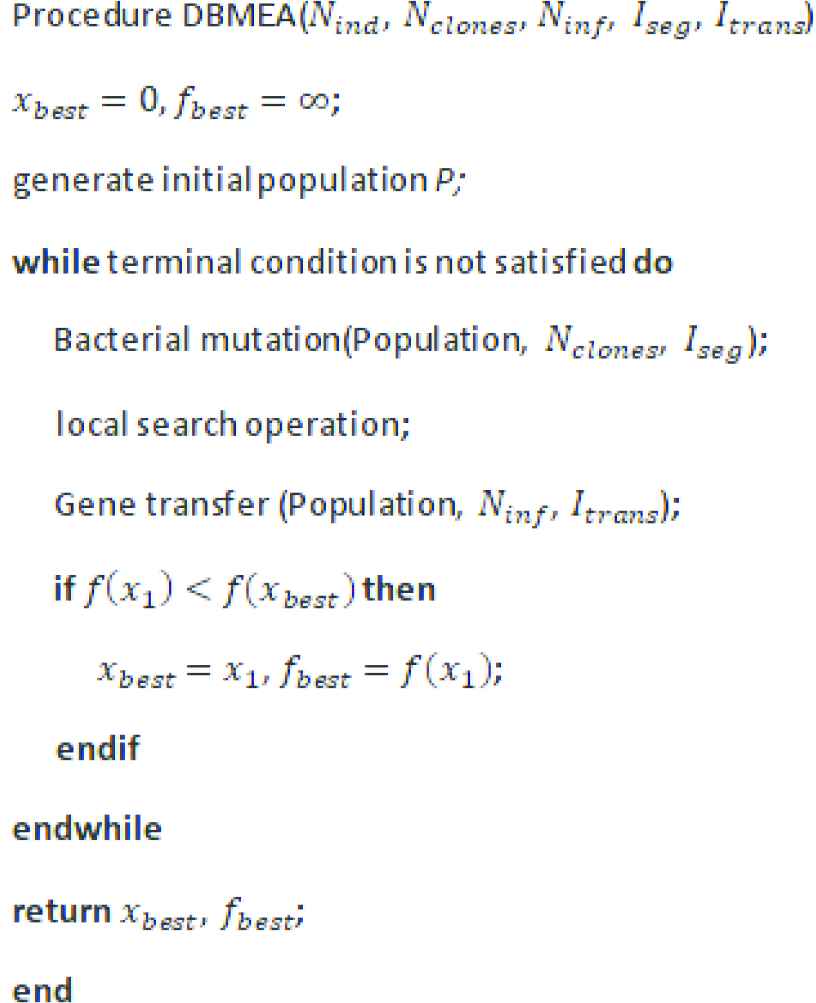
The pseudo-code of the DBMEA is given in Algorithm 1.
2.1. Creating the Initial Population
The “population” is the set of individuals each of which represents a possible solution to the problem. In this case they are the potential tours of the TRP.
In the DBMEA permutation encoding is used. Each city (graph node) is assigned to an index
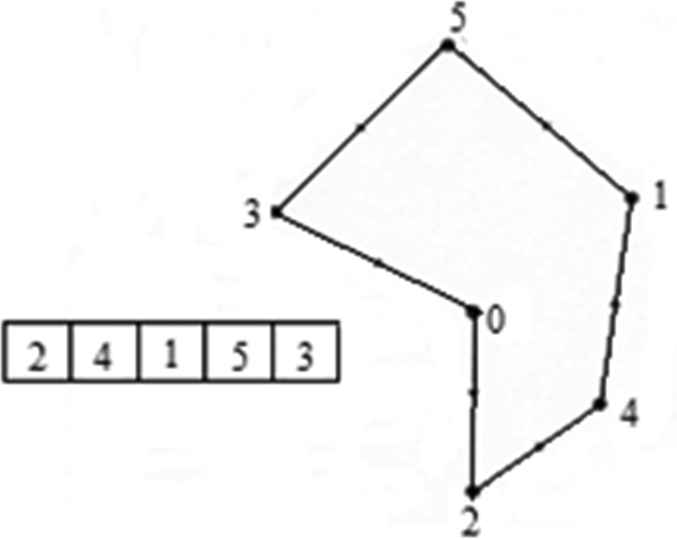
Encoding the individuals.
The initial population consists of randomly created individuals. Random creation ensures that the uniform distribution of the population in the search space is prevented from prematurely getting stuck into a local minimum.
Algorithm 1: Pseudo-code of the DBMEA.
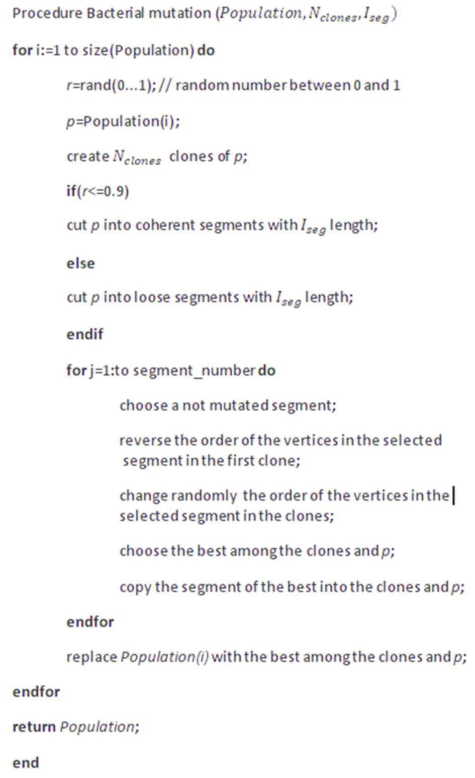
2.2. Bacterial Mutation
Bacterial mutation operates on the bacteria individually. The process of the bacterial mutation can be seen in Figure 2. For every bacterium of the population, the following process will be executed: Initially, a predefined number of clones
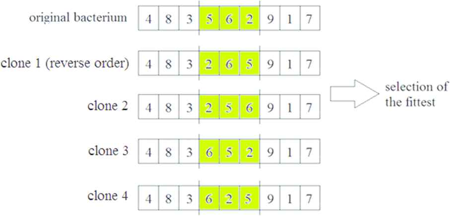
Bacterial mutation.
The next step is ranking the clones of the bacteria, including the original one, based on their fitness values. In the case of the TRP the evaluation of the clones is based on the Csum values (Equation 2). The mutated segment of the fittest clones is copied (back) to all the clones including the original bacterium. This process is consecutively applied until all the genes of the original bacterium have been mutated.
At the end of the mutation, the fittest clone is selected and it will replace the original bacterium, while the other clones are deleted. As a result, the remaining bacterium is at least as fit as the original bacterium.
Two different types of mutation are used in the algorithm, the coherent segment mutation and the loose segment mutation. Our experiments have shown that it is advantageous to use both in the algorithm.
Coherent segment mutation (Figure 3): in this case the elements of the segments are consecutive in the code.
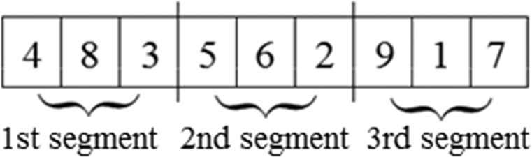
Coherent segment mutation.
Loose segment mutation (Figure 4): Opposed to coherent segment mutation, the segments of the bacterium do not need to consist of neighboring elements. It allows that the elements of the segments come from different parts of the bacterium. The time complexity of the bacterial mutation is
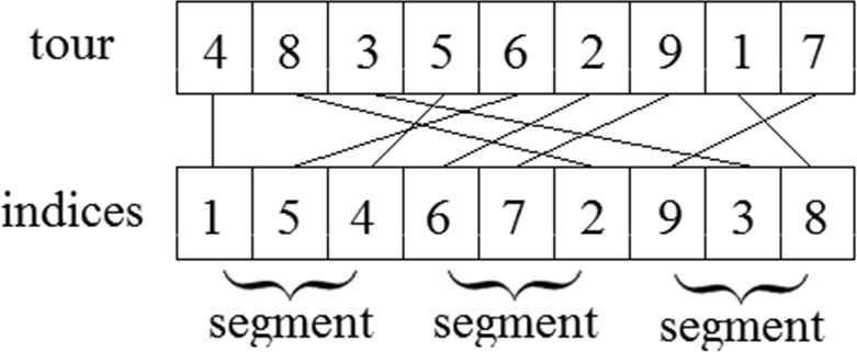
Loose segment mutation.
2.3. Local Search
Local search techniques form an important part of the memetic algorithms because combining an efficient local search with an evolutionary algorithm can increase the efficiency of the algorithm significantly [36].
A local search algorithm starts from a possible solution and then iterates in order to improve the neighborhood of the solution. In many optimization problems, it is advantageous to combine the local search with metaheuristics (genetic algorithms, BEAs, simulated annealing etc.).
Algorithm 2: Pseudo-code of the Bacterial mutation.
2.3.1. Combined local search for the TRP
The algorithm combines the 2-opt and 3-opt local search techniques in order to increase convergence speed. First the tour is improved with the 2-opt local steps and when no further improvement is possible with 2-opt, then the 3-opt search is applied. The local search is stopped when the tour cannot be improved further using the 3-opt steps. As a result of the local search the improved tour will be 3-optimal.
The process of local search for the TRP is more time consuming than for the TSP where the cost of the modified tour can be calculated from the cost of the original tour by adding the lengths (costs) of the newly added edges and subtracting the lengths of the deleted edges. For the TRP, it requires more calculations: Before starting the local search and after each improvement step of the tour, the arrival times and the sums of the arrival times need to be calculated for each node. Using these values the Csum (Equation 2) value of the tour after a local search step can be calculated requiring O(1) operations.
In the case of the TSP, the acceleration of the local search increased the efficiency of the DBMEA [31]. The TRP is in many respects similar to the TSP, so here, the same speed-up techniques were investigated in order to improve the performance of the algorithm for the TRP:
Candidate list [36]: It contains the indices of the closest vertices in ascending order and is created for all vertices. During the local search only the pre-defined number of closest vertices (contained in the candidate lists) are examined for each vertex because a shorter edge is more likely to be part of a high accuracy optimum solution.
“Don't look back bits” (dlb) [36]: Each vertex in assigned to a “don't look back bit.” If no improvement was found for a given vertex (v) then until an incident edge changes, do not consider v (this changes its “don't look back bit” to 1).
2.3.2. 2-opt local search
The 2-opt local search replaces two edge pairs in the original graph to reduce the length of the tour.
Two edge pairs (AB, CD) are iteratively replaced with AC and BD edges, which results in a new possible tour.
If the newly constructed tour has a lower cost than the edge pairs are exchanged; the edges AB and CD are deleted from the graph and edges AC and BD are inserted instead (Figure 5). One of the sub-tours between the original edges is reversed after the 2-opt move. This iterative process is terminated if no further improvement is possible.
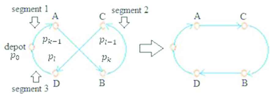
2-opt local search.
In the case of the 2-opt search, the tour falls into three segments, segment 1 goes from the depot to vertex A, segment 2 from vertex B to vertex C and segment 3 from vertex D back to the depot (Figure 5). The Csum value (Equation 2) of the new tour can be calculated using the following, requiring O(1) operations (Equation 3):
2.3.3. 3-opt local search
The 3-opt local search improves the tour by replacing three edges with three other ones. By removing three edges there are 8 alternative ways to reconnect the tour but four of them are identical with the corresponding 2-opt steps; thus they do not need to be examined here (Figure 6). The output of the 3-opt step is the least costly tour of all new tours.
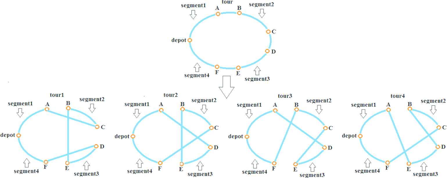
3-opt local search.
The calculation of the Csum values can be done similarly as above in the case of the 2-opt, the difference is that it is based on the total arrival times, total distances and number of vertices of four segments.
2.4. Gene Transfer
The gene transfer operation ensures the flow of information within the population, and hence results in better and better bacteria in the population.
First, the population is divided into two parts after sorting it in a descending order based on the fitness values. The “superior half” is the group of “good” bacteria, the “inferior half” is called “bad” bacteria. Next a predefined length (Itransfer) segment of a randomly selected “good” bacterium copies into a randomly selected “bad” bacterium in which the procedure is repeated Ninf times.
In Figure 7 the source segment is (6, 2, 9); and this segment is transferred to the destination bacterium (between 5 and 7). Double occurrences of nodes are eliminated, consequently the length of the bacterium remains
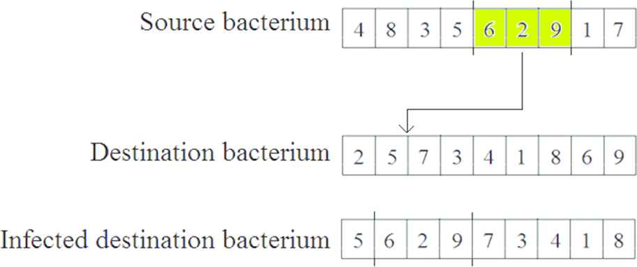
Gene transfer.
The time complexity of the gene transfer operation consists of three components:
The calculation time of fitness values
The sorting time of the population in a descending order, based on the fitness values
The calculation time of the new fitness value of the modified bacterium, and its reinsertion into the population gives
The total time complexity of the gene transfer operation in each generation (Equation 4) is
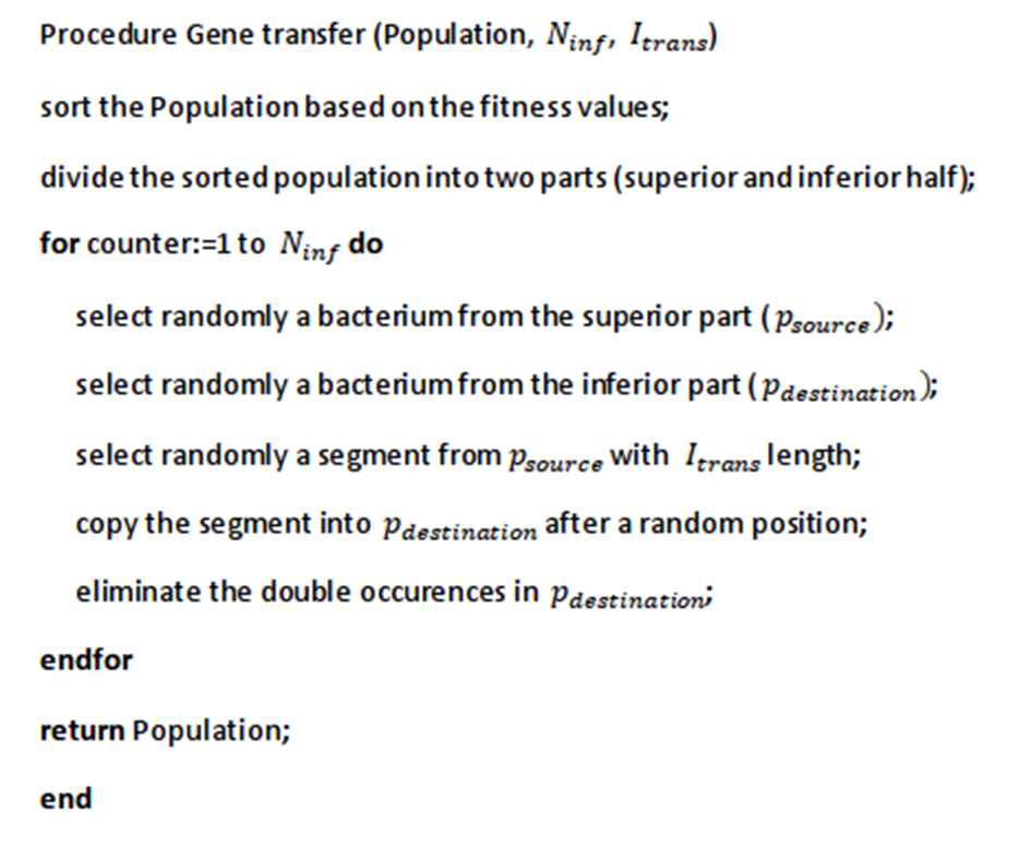
Algorithm 3 shows the pseudo-code of the Gene transfer operation.
3. COMPUTATIONAL RESULTS
The thus adapted DBMEA was tested on a series of benchmark problems, and each instance was ran 10 times. Our test results were compared to state-of-the-art heuristics, namely the
The GILS-RVND heuristic [19]
Salehipour et al.'s method [18]
Ngueveu et al.'s metaheuristic [20] methods, in order to prove the efficiency of the adapted DBMEA for solving the TRP. The mentioned heuristics were, however, tested on different hardware configurations, as namely
DBMEA: Intel Core i7-7500U 2.7 GHz, 8GB of RAM memory running under Linux Mint 18.2
GILS-RVND: Intel Core i7 2.93 GHz, 8 GB of RAM memory running under GNU/Linux Ubuntu 10.04
Salehipour et al.'s heuristic: Pentium 4, 2.4 GHz, 512 MB of RAM memory
Ngueveu et al.'s method: Pentium D 3.40 GHz, 1GB of RAM memory running under Windows XP
Algorithm 3: Pseudo-code of the Gene transfer.
The difference of hardwares has to be taken into consideration when doing the comparison.
Finding the optimal or quasi-optimal parameter values of an evolutionary algorithm is a crucial and time consuming task because the values of the parameters significantly affect the efficiency of the algorithm. For example, a small initial population size can cause that the algorithm fails to find good solutions because of the small diversity of the population, while the too big population size reduces the convergence speed. If the candidate lists of the local search are too short, it can be impossible to find the global optimum with the local search, however this search is fast.
In order to find the optimal parameters of the DBMEA brute force search was carried out. The following parameter values were tested, so in total 972 parameter configurations were tried out:
the number of bacteria in the population (Nind = 20, 50, 100, 200)
the number of clones in the bacterial mutation (Nclones = ncities/10, ncities/15, ncities/20)
the number of infections in the gene transfer (Ninf = 20, 40, 60)
the length of the chromosomes (Iseg = ncities/10, ncities/20, ncities/30)
the length of the transferred segment (Itrans = ncities/10, ncities/20, ncities/30)
length of the candidate lists
Each parameter configuration was tested on three benchmark instances (st70, lin 105, lin318) [43] with 5 test runs per each configuration.
We found that the best balance between the solution quality and the runtime resulting in high-quality solutions for both small and large instances was shown by the following configuration:
the number of bacteria in the population is (Nind = 100)
the number of clones in the bacterial mutationis (Nclones = ncities/15)
the number of infections in the gene transfer is (Ninf = 40)
the length of the chromosomes is (Iseg = ncities/20)
the length of the transferred segment is (Itrans = ncities/20)
the length of the candidate lists (square root of the number of cities)
For achieving a realistic comparison, the DBMEA was tested under both Windows 7 Professional and Linux Mint 18.2. We found that the execution was faster under Linux but the difference was not significant (see Table 1).
| Instance | DBMEA+2-opt+3-opt+cl+dlb |
|
|---|---|---|
| Average Sec. Linux Mint 18.2 | Average Sec. Windows 7 Professional | |
| berlin52 | 0.73 | 0.94 |
| st70 | 1.55 | 2.05 |
| lin105 | 5.15 | 6.24 |
| kroA100 | 3.66 | 4.41 |
| kroB100 | 6.34 | 8.43 |
DBMEA, Discrete Bacterial Memetic Evolutionary Algorithm.
Comparison of runtimes running under Linux and Windows.
The DBMEAs with different versions of local search were tested on the TSPLIB (TSP Library) benchmark instances [43]. In these cases the distance values are rounded to the closest integer value. For these instances, the optimal solutions were given by Abeledo et al. using the branch-cut-and-price algorithm [8]. We examined different speed-up techniques of local search for these instances and how they affected the solution qualities and the required runtimes. For all instances, the optimal solutions were found by all versions of the DBMEA, the speed-up techniques did not decrease the solution quality. The lowest runtimes were achieved using the DBMEA improved by the candidate lists search (cl) and “don't look back bit” speed-ups, which was on average 6.90 times faster than the DBMEA without speed-ups (Table 2). For the larger instances the version of the DMBEA that was used was called “DBMEA-best” (see Table 4–8).
| Instance | Best Known | DBMEA+2-opt+3-opt |
DBMEA+2-opt+3-opt+cl |
DBMEA+2-opt+3-opt+cl+dlb |
||||||||
|---|---|---|---|---|---|---|---|---|---|---|---|---|
| Best Value | Avg. Value | Avg. Sec | Best Value | Avg. Value | Avg. Sec | Ratio | Best Value | Avg. Value | Avg. Sec | Ratio | ||
| dantzig42 | 12528 | 12528 | 12528 | 0.56 | 12528 | 12528 | 0.19 | 2.95 | 12528 | 12528 | 0.15 | 3.73 |
| swiss42 | 22327 | 22327 | 22327 | 0.33 | 22327 | 22327 | 0.13 | 2.54 | 22327 | 22327 | 0.07 | 4.71 |
| att48 | 209320 | 209320 | 209320 | 2.80 | 209320 | 209320 | 0.76 | 3.68 | 209320 | 209320 | 0.48 | 5.83 |
| gr48 | 102378 | 102378 | 102378 | 1.81 | 102378 | 102378 | 0.57 | 3.18 | 102378 | 102378 | 0.42 | 4.31 |
| hk48 | 247926 | 247926 | 247926 | 1.04 | 247926 | 247926 | 0.38 | 2.74 | 247926 | 247926 | 0.31 | 3.35 |
| eil51 | 10178 | 10178 | 10178 | 3.24 | 10178 | 10178 | 1.01 | 3.21 | 10178 | 10178 | 0.75 | 4.32 |
| berlin52 | 143721 | 143721 | 143721 | 3.07 | 143721 | 143721 | 1.13 | 2.72 | 143721 | 143721 | 0.73 | 4.21 |
| brazil58 | 512361 | 512361 | 512361 | 1.96 | 512361 | 512361 | 0.56 | 3.50 | 512361 | 512361 | 0.50 | 3.92 |
| st70 | 20557 | 20557 | 20557 | 9.25 | 20557 | 20557 | 2.26 | 4.09 | 20557 | 20557 | 1.55 | 5.97 |
| eil76 | 17976 | 17976 | 17976 | 10.59 | 17976 | 17976 | 2.01 | 5.27 | 17976 | 17976 | 1.45 | 7.30 |
| pr76 | 3455242 | 3455242 | 3455242 | 7.54 | 3455242 | 3455242 | 1.64 | 4.60 | 3455242 | 3455242 | 0.99 | 7.62 |
| rat99 | 57986 | 57986 | 57986 | 64.30 | 57986 | 57986 | 10.28 | 6.25 | 57986 | 57986 | 9.99 | 6.44 |
| kroA100 | 983128 | 983128 | 983128 | 39.22 | 983128 | 983128 | 5.24 | 7.48 | 983128 | 983128 | 3.66 | 10.72 |
| kroB100 | 986008 | 986008 | 986008 | 53.92 | 986008 | 986008 | 6.92 | 7.79 | 986008 | 986008 | 6.34 | 8.50 |
| kroC100 | 961324 | 961324 | 961324 | 37.47 | 961324 | 961324 | 4.83 | 7.76 | 961324 | 961324 | 3.51 | 10.68 |
| kroD100 | 976965 | 976965 | 976965 | 40.70 | 976965 | 976965 | 5.73 | 7.10 | 976965 | 976965 | 4.55 | 8.95 |
| kroE100 | 971266 | 971266 | 971266 | 37.72 | 971266 | 971266 | 5.66 | 6.66 | 971266 | 971266 | 3.68 | 10.25 |
| rd100 | 340047 | 340047 | 340047 | 38.87 | 340047 | 340047 | 7.60 | 5.11 | 340047 | 340047 | 6.18 | 6.29 |
| eil101 | 27513 | 27513 | 27517.8 | 140.08 | 27513 | 27517.2 | 16.64 | 8.42 | 27513 | 27517.8 | 14.70 | 9.53 |
| lin105 | 603910 | 603910 | 603910 | 46.24 | 603910 | 603910 | 7.59 | 6.09 | 603910 | 603910 | 5.15 | 8.98 |
| pr107 | 2026626 | 2026626 | 2026626 | 36.74 | 2026626 | 2026626 | 6.41 | 5.73 | 2026626 | 2026626 | 3.92 | 9.37 |
DBMEA, Discrete Bacterial Memetic Evolutionary Algorithm; TSPLIB, Traveling Salesman Problem Library.
DBMEA results for the TSPLIB instances with various local searches.
Our results were compared with the GILS-RVND heuristic (Table 3). Both methods were tested on Linux. Both methods found the optimal solution for all instances but the DBMEA was in the majority of cases (15 out of 21) faster than the GILS-RVND heuristic even though the GILS-RVND was tested on hardware with a higher clock speed than the DBMEA (2.93 GHz vs. 2.7 GHz, with both Intel Core i7 processors).
| Instance | Best Known | DBMEA+2-opt+3-opt+cl+dlb |
GILS-RVND |
||||
|---|---|---|---|---|---|---|---|
| Best Value | Avg. Value | Avg. Sec | Best Value | Avg. Value | Avg. Sec | ||
| dantzig42 | 12528 | 12528 | 12528 | 0.15 | 12528 | 12528 | 0.16 |
| swiss42 | 22327 | 22327 | 22327 | 0.07 | 22327 | 22327 | 0.16 |
| att48 | 209320 | 209320 | 209320 | 0.48 | 209320 | 209320 | 0.32 |
| gr48 | 102378 | 102378 | 102378 | 0.42 | 102378 | 102378 | 0.33 |
| hk48 | 247926 | 247926 | 247926 | 0.31 | 247926 | 247926 | 0.3 |
| eil51 | 10178 | 10178 | 10178 | 0.75 | 10178 | 10178 | 0.49 |
| berlin52 | 143721 | 143721 | 143721 | 0.73 | 143721 | 143721 | 0.46 |
| brazil58 | 512361 | 512361 | 512361 | 0.50 | 512361 | 512361 | 0.78 |
| st70 | 20557 | 20557 | 20557 | 1.55 | 20557 | 20557 | 1.65 |
| eil76 | 17976 | 17976 | 17976 | 1.45 | 17976 | 17976 | 2.64 |
| pr76 | 3455242 | 3455242 | 3455242 | 0.99 | 3455242 | 3455242 | 2.31 |
| rat99 | 57986 | 57986 | 57986 | 9.99 | 57986 | 57986 | 11.27 |
| kroA100 | 983128 | 983128 | 983128 | 3.66 | 983128 | 983128 | 8.59 |
| kroB100 | 986008 | 986008 | 986008 | 6.34 | 986008 | 986008 | 9.21 |
| kroC100 | 961324 | 961324 | 961324 | 3.51 | 961324 | 961324 | 8.17 |
| kroD100 | 976965 | 976965 | 976965 | 4.55 | 976965 | 976965 | 8.46 |
| kroE100 | 971266 | 971266 | 971266 | 3.68 | 971266 | 971266 | 8.31 |
| rd100 | 340047 | 340047 | 340047 | 6.18 | 340047 | 340047 | 8.52 |
| eil101 | 27513 | 27513 | 27517.8 | 14.0 | 27513 | 27513 | 12.76 |
| lin105 | 603910 | 603910 | 603910 | 5.15 | 603910 | 603910 | 8.42 |
| pr107 | 2026626 | 2026626 | 2026626 | 3.92 | 2026626 | 2026626 | 10.89 |
Instances selected by Abeledo et al. [8].
DBMEA, Discrete Bacterial Memetic Evolutionary Algorithm; TSPLIB, Traveling Salesman Problem Library.
Comparison of results for TSPLIB instances.a
Our results were compared with the GILS-RVND heuristic (Table 3). Both methods were tested under Linux. The best version of the DBMEA (see Table 2) was also tested on the same TSPLIB instances, which were selected by Salehipour et al. Some of these instances can also be found in Tables 2 and 3, but here, the solutions are different. The differences are caused by the different objective functions. In this case the values of the cost matrix are rounded to the next smallest integer and the sum of the arrival time does not contain the arrival time at the depot.
In Table 4, the results of the most efficient version of the DBMEA are compared with the GILS-RVND heuristic and the method used by Salehipour et al. The best and average values of the other methods are compared to the results of the DBMEA in the “Gap” columns with the following equations (Equation 5):
| Instance | Best Known | DBMEA-best |
GILS-RVND |
Salehipour et al. |
Gap (%) GILS-RVND |
Gap (%) Salehipour et al. |
|||
|---|---|---|---|---|---|---|---|---|---|
| Best Value | Avg. Value | Best Value | Avg. Value | Best Value | Best Value | Avg. Value | Best Value | ||
| st70 | 19215 | 19215 | 19215 | 19215 | 19215 | 19553 | 0.00 | 0.00 | −1.73 |
| rat99 | 54984 | 54984 | 54984 | 54984 | 54984 | 56994 | 0.00 | 0.00 | −3.53 |
| kroD100 | 949594 | 949594 | 949594 | 949594 | 949594 | 976830 | 0.00 | 0.00 | −2.79 |
| lin105 | 585823 | 585823 | 585823 | 585823 | 585823 | 585823 | 0.00 | 0.00 | 0.00 |
| pr107 | 1980767 | 1980767 | 1980767 | 1980767 | 1980767 | 1983475 | 0.00 | 0.00 | −0.14 |
| rat195 | 210191 | 210191 | 210284.3 | 210191 | 210335.9 | 213371 | 0.00 | −0.02 | −1.49 |
| pr226 | 7100308 | 7100308 | 7100308 | 7100308 | 7100308 | 7226554 | 0.00 | 0.00 | −1.75 |
| lin318 | 5560679 | 5562148 | 5566344.8 | 5560679 | 5569820 | 5876537 | 0.03 | −0.06 | −5.35 |
| pr439 | 17688561 | 17693137 | 17710528 | 17688561 | 17734922 | 18567170 | 0.03 | −0.14 | −4.70 |
| att532 | 5581240 | 5579113 | 5584915.3 | 5581240 | 5597867 | –b | −0.04 | −0.23 | – |
Instances selected by Salehipour et al. [18].
The distances between the nodes were calculated in Euclidean distances instead of ATT pseudo-Euclidean distances, so the results are not comparable.
DBMEA, Discrete Bacterial Memetic Evolutionary Algorithm; TSPLIB, Traveling Salesman Problem Library.
Solutions for TSPLIB instances.a
The negative values in these columns indicate where DBMEA found better results.
The DBMEA found much better solutions than Salehipour et al. (see the last column in Table 4). In most cases the DBMEA found the same (best known) solutions as the GILS-RVND heuristic. Although in the case of two instances (lin318, pr439) the GILS-RVND found a somewhat lower value for the optimum but the average optimal values were higher than the ones obtained using the DBMEA. It means that in a single run, the DBMEA is more likely to find a “good” solution than the GILS-RVND heuristic. For att532 the DBMEA found a new best solution. Thus, DBMEA outperformed both other methods in terms of runtime (Figure 8).
Comparison of runtimes for Traveling Salesman Problem Library (TSPLIB) instances.
A large instance set was generated by Salehipour et al., which contained seven different problem sizes ranging from 10 to 1000 vertices (10, 20, 50, 100, 200, 500, 1000) with 20 random instances for each problem size [34]. The coordinates were generated from a uniform distribution.
For small instances (10, 20 50) all three methods, the DBMEA, the heuristics of Salehipour et al. and the GILS-RVND found the optimal solutions (Table 5). In the case of the DBMEA, both the best values and the average values were the same (in the case of all runs the optimal value was found). The results for instances with sizes of 100 and 200 are not detailed in the paper because the DBMEA found very similar, almost equal values to the GILS-RVND heuristic.
| Instance | DBMEA-best |
Optimal Value |
||||
|---|---|---|---|---|---|---|
| S10 | S20 | S50 | S10 | S20 | S50 | |
| TRP-Sn-R1 | 1303 | 3175 | 12198 | 1303 | 3175 | 12198 |
| TRP-Sn-R2 | 1517 | 3248 | 11621 | 1517 | 3248 | 11621 |
| TRP-Sn-R3 | 1233 | 3570 | 12139 | 1233 | 3570 | 12139 |
| TRP-Sn-R4 | 1386 | 2983 | 13071 | 1386 | 2983 | 13071 |
| TRP-Sn-R5 | 978 | 3248 | 12126 | 978 | 3248 | 12126 |
| TRP-Sn-R6 | 1477 | 3328 | 12684 | 1477 | 3328 | 12684 |
| TRP-Sn-R7 | 1163 | 2809 | 11176 | 1163 | 2809 | 11176 |
| TRP-Sn-R8 | 1234 | 3461 | 12910 | 1234 | 3461 | 12910 |
| TRP-Sn-R9 | 1402 | 3475 | 13149 | 1402 | 3475 | 13149 |
| TRP-Sn-R10 | 1388 | 3359 | 12892 | 1388 | 3359 | 12892 |
| TRP-Sn-R11 | 1405 | 2916 | 12103 | 1405 | 2916 | 12103 |
| TRP-Sn-R12 | 1150 | 3314 | 10633 | 1150 | 3314 | 10633 |
| TRP-Sn-R13 | 1531 | 3412 | 12115 | 1531 | 3412 | 12115 |
| TRP-Sn-R14 | 1219 | 3297 | 13117 | 1219 | 3297 | 13117 |
| TRP-Sn-R15 | 1087 | 2862 | 11986 | 1087 | 2862 | 11986 |
| TRP-Sn-R16 | 1264 | 3433 | 12138 | 1264 | 3433 | 12138 |
| TRP-Sn-R17 | 1058 | 2913 | 12176 | 1058 | 2913 | 12176 |
| TRP-Sn-R18 | 1083 | 3124 | 13357 | 1083 | 3124 | 13357 |
| TRP-Sn-R19 | 1394 | 3299 | 11430 | 1394 | 3299 | 11430 |
| TRP-Sn-R20 | 951 | 2796 | 11935 | 951 | 2796 | 11935 |
Instances generated by Salehipour et al. [18].
DBMEA, Discrete Bacterial Memetic Evolutionary Algorithm; TRP, Traveling Repairman Problem.
Solutions for small instances.a
In the case of the size of 500, the DBMEA performed much better than the GILS-RVND. For the 13 instances with the size of 500 the DBMEA found new best values, and the average values were better, except in one case (R14) (see Table 6). On the average, the best cost was less by 0.06%, while the average cost by 0.35% than in the case of applying the GILS-RVND for instances of 500 nodes. In terms of runtimes, in most cases the DBMEA was also better than the GILS-RVND.
| Instance | DBMEA-best |
GILS-RVND |
Gap (%) GILS-RVND |
|||||
|---|---|---|---|---|---|---|---|---|
| Best | Average | Time (s) | Best | Average | Time (s) | Best | Average | |
| TRP-S500-R1 | 1843642 | 1846154 | 1530.15 | 1841386 | 1856018.7 | 1738.48 | 0.12 | −0.53 |
| TRP-S500-R2 | 1819357 | 1820603.3 | 1363.97 | 1816568 | 1823196.9 | 1476.13 | 0.15 | −0.14 |
| TRP-S500-R3 | 1825944 | 1826183.3 | 1421.18 | 1833044 | 1839254.2 | 1557.48 | −0.39 | −0.72 |
| TRP-S500-R4 | 1807676 | 1809097 | 1657.47 | 1809266 | 1815876.4 | 1597.06 | −0.09 | −0.37 |
| TRP-S500-R5 | 1823243 | 1823943 | 1496.96 | 1823975 | 1834031.7 | 1530.94 | −0.04 | −0.55 |
| TRP-S500-R6 | 1785596 | 1789337.5 | 1535.24 | 1786620 | 1790912.4 | 1576.91 | −0.06 | −0.09 |
| TRP-S500-R7 | 1846547 | 1846915 | 1521.77 | 1847999 | 1857926.6 | 1584.67 | −0.08 | −0.60 |
| TRP-S500-R8 | 1819792 | 1820467 | 1505.08 | 1820846 | 1829257.3 | 1565.01 | −0.06 | −0.48 |
| TRP-S500-R9 | 1731478 | 1731810.7 | 1196.69 | 1733819 | 1737024.9 | 1409.23 | −0.14 | −0.30 |
| TRP-S500-R10 | 1761221 | 1763814.8 | 1297.97 | 1762741 | 1767366.3 | 1621.85 | −0.09 | −0.20 |
| TRP-S500-R11 | 1797758 | 1799535.8 | 1603.76 | 1797881 | 1801467.9 | 1530.98 | −0.01 | −0.11 |
| TRP-S500-R12 | 1775801 | 1776487 | 1404.47 | 1774452 | 1783847.1 | 1554.75 | 0.08 | −0.41 |
| TRP-S500-R13 | 1865528 | 1869326.3 | 1540.7 | 1873699 | 1878049.4 | 1598.46 | −0.44 | −0.47 |
| TRP-S500-R14 | 1804917 | 1806526.8 | 1588.03 | 1799171 | 1805732.9 | 1701.9 | 0.32 | 0.04 |
| TRP-S500-R15 | 1786699 | 1790030.7 | 1370.71 | 1791145 | 1797532.9 | 1623.79 | −0.25 | −0.42 |
| TRP-S500-R16 | 1808327 | 1813399.5 | 1590.09 | 1810188 | 1816484 | 1583.7 | −0.10 | −0.17 |
| TRP-S500-R17 | 1820921 | 1823962.3 | 1619.62 | 1825748 | 1834443.2 | 1549.8 | −0.27 | −0.57 |
| TRP-S500-R18 | 1829993 | 1831120.3 | 1445.56 | 1826263 | 1833323.7 | 1620.02 | 0.20 | −0.12 |
| TRP-S500-R19 | 1777407 | 1778580.3 | 1480.87 | 1779248 | 1782763.9 | 1602.87 | −0.10 | −0.24 |
| TRP-S500-R20 | 1822243 | 1822325 | 1346.66 | 1820813 | 1830483.3 | 1507.96 | 0.08 | −0.45 |
Instances generated by Salehipour et al. [18].
DBMEA, Discrete Bacterial Memetic Evolutionary Algorithm; TRP, Traveling Repairman Problem.
Solutions for instances with 500 nodes.a
For instances with the size of 1000, the DBMEA also outperformed the GILS-RVND heuristic. For 19 instances with the size of 1000, the DBMEA found new best solutions (on the average, 0.40% better), and the average values were in all cases better (on the average, by 0.57%) compared to the GILS-RVND heuristic (see Table 7).
| Instance | DBMEA-best |
GILS-RVND |
Gap [%] GILS-RVND |
|||||
|---|---|---|---|---|---|---|---|---|
| Best | Average | Time (s) | Best | Average | Time (s) | Best | Average | |
| TRP-S1000-R1 | 5082586 | 5089863 | 13203.51 | 5107395 | 5133698.3 | 31894.51 | −0.49 | −0.86 |
| TRP-S1000-R2 | 5081789 | 5091883.8 | 15705.61 | 5106161 | 5127449.4 | 30881.19 | −0.48 | −0.70 |
| TRP-S1000-R3 | 5089622 | 5103438.2 | 15734.9 | 5096977 | 5113302.9 | 30184.15 | −0.14 | −0.19 |
| TRP-S1000-R4 | 5100544 | 5112470 | 15125.82 | 5118006 | 5141392.6 | 29951.12 | −0.34 | −0.57 |
| TRP-S1000-R5 | 5085208 | 5088281.4 | 14953.62 | 5103894 | 5122660.7 | 30129.51 | −0.37 | −0.68 |
| TRP-S1000-R6 | 5116794 | 5122238.8 | 15130.3 | 5115816 | 5143087.1 | 28161.57 | 0.02 | −0.41 |
| TRP-S1000-R7 | 4968048 | 4993075 | 15199.74 | 5021383 | 5032722 | 25945.41 | −1.07 | −0.79 |
| TRP-S1000-R8 | 5102829 | 5118066.4 | 15249.06 | 5109325 | 5132722.6 | 26572.71 | −0.13 | −0.29 |
| TRP-S1000-R9 | 5025037 | 5032504.8 | 14349.58 | 5052599 | 5073245.3 | 26330.4 | −0.55 | −0.81 |
| TRP-S1000-R10 | 5056106 | 5063444 | 14816.43 | 5078191 | 5093592.6 | 25676.31 | −0.44 | −0.60 |
| TRP-S1000-R11 | 5033519 | 5047486.3 | 14915.43 | 5041913 | 5066161.5 | 26235.63 | −0.17 | −0.37 |
| TRP-S1000-R12 | 5010741 | 5030020 | 15029.06 | 5029792 | 5051235.2 | 27910.11 | −0.38 | −0.42 |
| TRP-S1000-R13 | 5081275 | 5092837.4 | 15300.22 | 5102520 | 5131437.5 | 28475.89 | −0.42 | −0.76 |
| TRP-S1000-R14 | 5067053 | 5080584.8 | 15659.94 | 5099433 | 5118980.6 | 27639.81 | −0.64 | −0.76 |
| TRP-S1000-R15 | 5130957 | 5155507 | 15281.32 | 5142470 | 5174493.2 | 27633.07 | −0.22 | −0.37 |
| TRP-S1000-R16 | 5039840 | 5046737.8 | 14878.18 | 5073972 | 5090280.5 | 26653.16 | −0.68 | −0.86 |
| TRP-S1000-R17 | 5048305 | 5057721 | 15124.37 | 5071485 | 5084450.4 | 27503.43 | −0.46 | −0.53 |
| TRP-S1000-R18 | 4998682 | 5014361.7 | 15483.35 | 5017589 | 5037094 | 28808.09 | −0.38 | −0.45 |
| TRP-S1000-R19 | 5054659 | 5058987.7 | 14927.27 | 5076800 | 5097167.6 | 29637.49 | −0.44 | −0.75 |
| TRP-S1000-R20 | 4968394 | 4989050.3 | 1322.53 | 4977262 | 5002920.6 | 27499.24 | −0.18 | −0.28 |
Instances generated by Salehipour et al. [18].
DBMEA, Discrete Bacterial Memetic Evolutionary Algorithm; TRP, Traveling Repairman Problem.
Solutions for instances with 1000 nodes.a
The papers on the methods of Salehipour et al. and Ngueveu et al. contain only the average results (comparing the upper bounds) of 20 instances per problem size. The upper bounds were calculated with the nearest neighbor heuristic. In order to compare them with the DBMEA, the average gaps to the upper bounds needed to be calculated. The summarized results can be found in Table 8. The DBMEA was also much better in terms of solution quality and runtime compared to both the heuristics of Salehipour et al. and Ngueveu et al. (although both methods have several versions, always the versions producing the lowest values were chosen for comparison). In addition, the heuristics of Salehipour et al. and Ngueveu et al. were unable at all to solve the largest of the instances (with the size of 1000) within any reasonable runtime using these specified configurations.
| Size | DBMEA-best |
GILS-RVNS |
Ngueveu et al. |
Salehipour et al. |
||||
|---|---|---|---|---|---|---|---|---|
| Upper Bound (%) | Time (s) | Upper Bound (%) | Time (s) | Upper Bound (%) | Time (s) | Upper Bound (%) | Time (s) | |
| 10 | −2.44 | 0.00 | −2.44 | 0.00 | −2.43 | 0.00 | −2.44 | 0.00 |
| 20 | −10.28 | 0.02 | −10.28 | 0.02 | −10.11 | 0.01 | −9.86 | 0.04 |
| 50 | −11.01 | 0.69 | −11.01 | 0.55 | −9.36 | 1.44 | −9.74 | 3.54 |
| 500 | −15.45 | 1475.85 | −15.16 | 1576.6 | −13.85 | 16208.7 | −9.71 | 10381.36 |
| 1000 | −15.95 | 15069.51 | −15.47 | 28186.14 | – | – | – | – |
DBMEA, Discrete Bacterial Memetic Evolutionary Algorithm.
Summarizing the results for the instance set generated by Salehipour et al. [18].
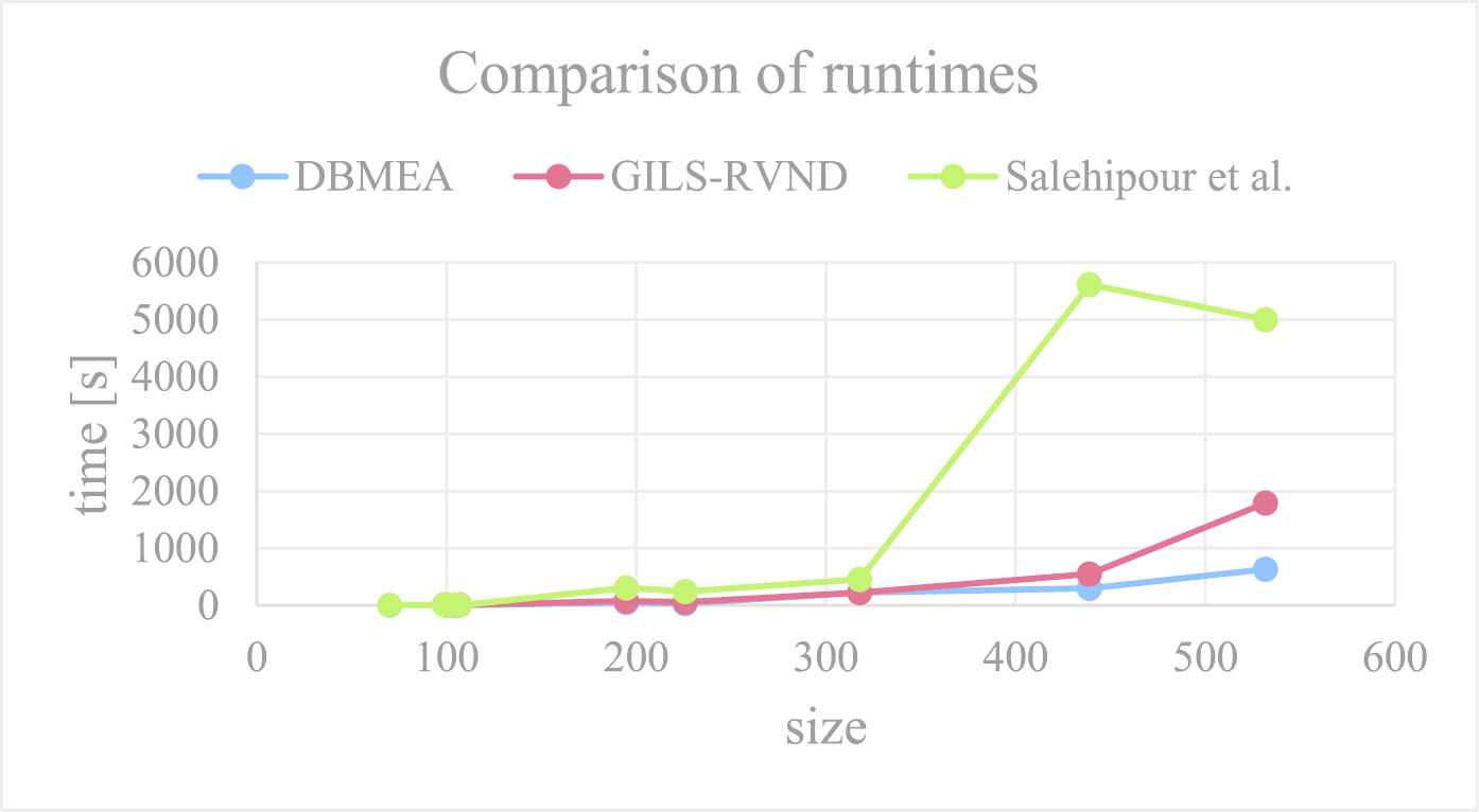
With a growing problem size, the DBMEA also became more efficient than the GILS-RVND heuristic. For instances with sizes of 500 and 1000, our proposed new heuristic always found better values while having lower runtimes (Figure 9).
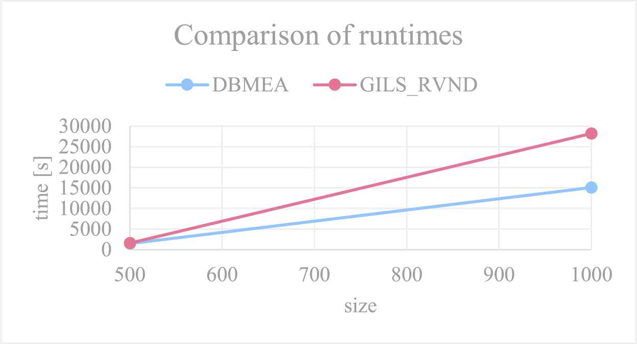
Comparison of runtimes for instances generated by Salehipour et al. [18].
4. THE ANALYSIS OF THE AVAILABLE METAHEURISTICS
The efficiency of the DBMEA and the GILS-RVND heuristic was compared with statistical methods.
The following models were fitted to the mean run times of each method:
polynomial:
exponential:
square-root exponential:
A curve which minimizes the root mean square error (RMSE) was fitted to the mean values of the run times.
Table 9 shows the parameters of the curves of both algorithms fitted as mentioned before. The DBMEA has the lowest b parameter value, which fact indicates that it will be faster on large instances than the former most efficient heuristic, the GILS-RVND.
| a | b | ||
|---|---|---|---|
| GILS-RVND | Polynomial | 9.44*10−9 | 4.1583 |
| Exponential | 77.77089 | 1.00591 | |
| Square-root Exponential | 1.4661 | 1.366 | |
| DBMEA | Polynomial | 0.00000138 | 3.3458 |
| Exponential | 114.2444 | 1.00489 | |
| Square-root Exponential | 5.1519 | 1.2871 |
Parameters of the fitting models.
Table 10 shows the RMSE and R2-values of the fitting models. Because of the low number of points, the R2-values are very close to 1 in each case, so the run time predictability cannot be evaluated due to the limited amount of test data.
| RMSE | R2 | ||
|---|---|---|---|
| GILS-RVND | Polynomial | 18.81 | 1 |
| Exponential | 139.5 | 0.99999 | |
| Square-root Exponential | 28.71 | 1 | |
| DBMEA | Polynomial | 29.03 | 1 |
| Exponential | 176.3 | 0.999 | |
| Square-root Exponential | 42.41 | 0.999 |
RMSE, root mean square error.
The RMSE and R2-value of the fitting models.
5. CONCLUSIONS
In this paper, an efficient metaheuristic, the improved DBMEA adapted for the TRP problem, was introduced in order to solve the TRP. The efficiency of the method was shown by testing it on a large number of instances, up to 1000 vertices. It can be concluded that the DBMEA has better properties both in terms of solution quality and runtime compared to the most efficient methods known so far. This is especially true for large instances (with at least 500 vertices) in which the DBMEA found new “best solutions” at the same time having lower runtimes. The runtime properties of the DBMEA and the state-of-the-art GILS-RVND heuristic were compared by applying curve fitting. The parameter values of the fitted curves show that the DBMEA is a faster method than the so far best GILS-RVND heuristic.
Based on the above-presented test results we recommend using the DBMEA to solve the TRP in general, especially for large instances.
CONFLICT OF INTEREST
The Authors declare that there is no conflict of interest.
AUTHORS' CONTRIBUTIONS
The authors contributed equally to this work.
Funding Statement
The work was supported by the GINOP-2.3.4-15-2016-00003 project.
ACKNOWLEDGMENTS
This work was supported by the National Research, Development and Innovation Office (NKFIH) K124055.
 Supported by the ÚNKP-18-3 New National Excellence Program of the Ministry of Human Capacities. The work was supported by EFOP-3.6.2-16-2017-00015 HU-MATHS-IN – Intensification of the activity of the Hungarian Industrial Innovation Mathematical Service Network.
REFERENCES
Cite this article
TY  - JOUR
AU  - Boldizsár Tüű-Szabó
AU  - Péter Földesi
AU  - László T. Kóczy
PY  - 2020
DA  - 2020/06/16
TI  - An Efficient Evolutionary Metaheuristic for the Traveling Repairman (Minimum Latency) Problem
JO  - International Journal of Computational Intelligence Systems
SP  - 781
EP  - 793
VL  - 13
IS  - 1
SN  - 1875-6883
UR  - https://doi.org/10.2991/ijcis.d.200529.001
DO  - 10.2991/ijcis.d.200529.001
ID  - Tüű-Szabó2020
ER  -