
A Neural Network for Moore–Penrose Inverse of Time-Varying Complex-Valued Matrices
 , Jiqiang Feng1
- DOI
- 10.2991/ijcis.d.200527.001How to use a DOI?
- Keywords
- Zhang neural network; Moore–Penrose inverse; Finite-time convergence; Noise suppression
- Abstract
The Moore–Penrose inverse of a matrix plays a very important role in practical applications. In general, it is not easy to immediately solve the Moore–Penrose inverse of a matrix, especially for solving the Moore–Penrose inverse of a complex-valued matrix in time-varying situations. To solve this problem conveniently, in this paper, a novel Zhang neural network (ZNN) with time-varying parameter that accelerates convergence is proposed, which can solve Moore–Penrose inverse of a matrix over complex field in real time. Analysis results show that the state solutions of the proposed model can achieve super convergence in finite time with weighted sign-bi-power activation function (WSBP) and the upper bound of the convergence time is calculated. A related noise-tolerance model which possesses finite-time convergence property is proved to be more efficient in noise suppression. At last, numerical simulation illustrates the performance of the proposed model as well.
- Copyright
- © 2020 The Authors. Published by Atlantis Press SARL.
- Open Access
- This is an open access article distributed under the CC BY-NC 4.0 license (http://creativecommons.org/licenses/by-nc/4.0/).
1. INTRODUCTION
The Moore–Penrose inverse of a matrix is widely used in scientific and engineering fields as one of the basic problems encountered extensively, such as pattern recognition [1], optimization [2], and signal processing [3]. In general, it is not easy to immediately and accurately solve the Moore–Penrose inverse in numerical simulation. Because of its wide applications, the calculation of Moore–Penrose inverse has been studied a lot, and many algorithms for constant matrix have been proposed, such as continuous matrix square algorithm [4], Newton iteration method [5] and Greyville recursion [6]. However, in the process of solving matrix inverse kinematics problems of online control of redundant robots [7], the real-time calculation problem of the matrix Moore–Penrose inverse is required to be solved. Although there have been many effective methods for solving the matrix Moore–Penrose inverse, as far as we know, most of the research is based on the real field and few people generalize this problem to the complex field. In fact, solving the Moore–Penrose inverse of the complex-valued matrix is also often involved in the abovementioned fields, and it also plays a pivotal role in practical applications.
Parallel computing is widely used to solve linear and nonlinear problems [7–16] for its superior performance in complex large-scale online applications. Neural network is considered as an effective alternative to scientific computing [17,18] due to its parallel distribution and easy hardware implementation. Some recursive neural networks [19–21] have been constructed to compute the pseudo-inverse of matrices.
Zhang neural network (ZNN), as a special kind of recurrent neural network, is different from gradient neural networks (GNNs) that use a passive tracking method. ZNN performs better when involving the time derivative information of time-varying coefficients. It has the advantages of fast convergence rate in solving time-varying problems. And it is widely used in dynamic problems such as nonlinear dynamic optimization [22], motion control of robot redundant arms [23]. In 2013, a sign-bi-power activation function that accelerates ZNN to converge in finite time was proposed by Li et al. [24]. Then, Shen et al. [25] tried to accelerate the convergence rate of ZNN by constructing a tunable activation function. In addition, robustness is also an influence property because noise interference is unavoidable in practical application. Thus, inspired by xiao et al. [26], one noise-tolerance ZNN model which possesses finite-time convergence property is proposed in this paper.
It has been shown that ZNN has been proven to own superior property in many studies (see [27–29]). Therefore, for the time-varying full-rank matrix Moore–Penrose inversion problem, we choose to construct a ZNN to solve the time-varying optimization problem. The contributions of this paper are listed as follows:
To the best of our knowledge, there is little research on solving time-varying Moore–Penrose inverse problems over complex field with ZNN model. Compared with the existing results [30], we generalize the problem to the complex field and solve the Moore–Penrose inverse in finite time.
A time-varying parameter is utilized in the design formula, which can effectively reduce the convergence time of the model solution.
An improved ZNN model which is proved to be more efficient in noise suppression compared with traditional ZNN model is proposed, and the value of its error function converges to zero in finite time.
The remains of this paper are summarized as follows: Some definitions and preliminaries about generalized inverse and complex analysis are introduced in Section 2. The ZNN model for right Moore–Penrose inverse of a matrix with special activation function is constructed and its Lyapunov stability and convergence in finite time are proved in Section 3. In addition, an improved ZNN model for matrix Moore–Penrose inverse which has the ability to suppress noise is introduced. It is worth mentioning that the improved ZNN model can not only effectively suppress noise but also its solution can reach a finite time convergence under the acceleration of a special activation function. In Section 4, numerical examples of time-vary complex-valued problems are given to demonstrate the validity of our results.
2. PROBLEM DESCRIPTION AND PRELIMINARIES
In order to lay the foundation for further discussion, some definitions about the matrix Moore–Penrose inverse are introduced. In this paper,
Definition 1.
[7,31] For a matrix
If
From (1), the Moore–Penrose inverse of matrix
From the definition of
Proposition 1.
[32] For any
3. MODEL DESIGN AND CONVERGENCE ANALYSIS
In this section, we will propose a ZNN model and an improved noise-tolerance ZNN model to solve right time-varying Moore–Penrose inverse of matrices. Their stability and convergence are discussed as well.
3.1. A ZNN Model for Right Time-Varying Moore–Penrose Inverse
In this subsection, we will propose a ZNN model to solve the right Moore–Penrose inverse of time-varying matrix
For solving
The corresponding error function [8,33] could be defined as
Here
Combining (3) with (4), ZNN model is written as follows:
Theorem 2.
For any nonzero complex-valued activation function array
Proof.
For convenience, design formula (4) could be written as subsystems:
The Lyapunov function is defined as
The derivative with respect to time is
Since
So we can get that
It is worth mentioning that under the acceleration of time-varying parameter
Theorem 3.
From any initial value
Proof.
For the Lyapunov function
That is,
From the above inequality, we can conclude that
Integrating both sides of this inequality from
Since
Therefore,
The upper bound on the convergence time of
As is proved above, the state solution of ZNN model can converge to the theoretical solution
It is worth noting that compared with the methods proposed in other references [8,30], not only do we generalize the problem to the complex domain, but also the state solution of the model proposed in this paper can achieve finite time convergence.
Remark 1.
ZNN model for left time-varying Moore–Penrose inverse of matrices can be obtained similarly. The error function could be defined as
The convergence analysis is similar to the proof of Theorems 2 and 3, thus omitted here.
3.2. An Improved Matrix Inversion ZNN Model
The analysis about ZNN model for right time-varying Moore–Penrose inverse in Section 3.1 does not concern the problem of external noise, which means the state solution of the ZNN model (7) and (12) may be unstable once the external noise appears. In this section, we propose an improved matrix inversion ZNN model which can also be more efficient in noise suppression.
We introduce a design formula [26] for
The following theorem ensures the state solution of the ZNN model (14) converges to the exact solution in finite time.
Theorem 4.
From any initial state
Proof.
We firstly introduce an intermediate variable
Define a Lyapunov function as
Note that
It is similar to (8). According to the proof of Theorem 2,
Next, the upper bound of convergent time of state solution
Theorem 5.
Starting from any initial state
Proof.
According to (15), we can further get
Multiplying
Thus, we get
To verify noise-tolerance ability, we add a constant external noise to design formula (13) which is denoted by
Theorem 6.
For noise-polluted model (18), the state solution
Proof.
As defined in Theorem 4,
Define a Lyapunov function as
It is obvious that
That is to say,
4. NUMERICAL EXAMPLES
In this section, numerical examples are presented to illustrate the effectiveness of the proposed ZNN model.
Example 1.
Consider the right Moore–Penrose inverse of the following complex time-varying matrix:
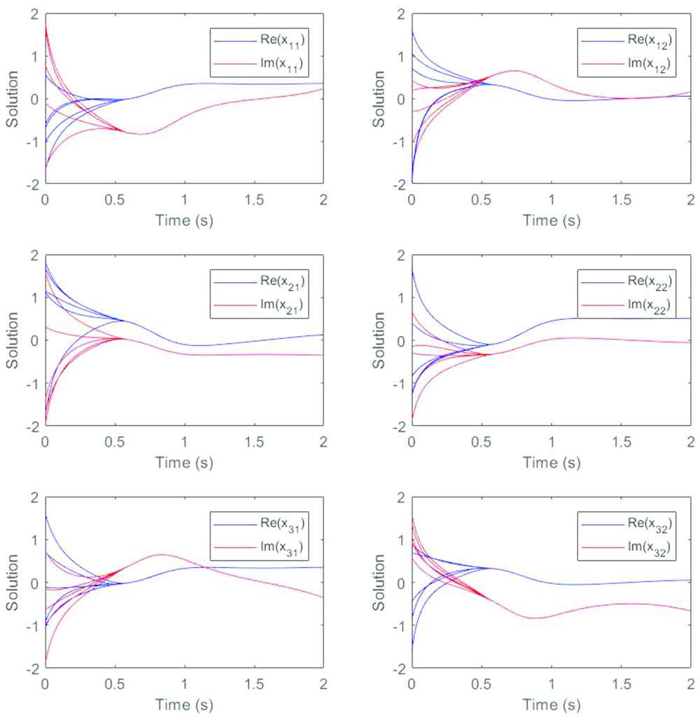
The Zhang neural network (ZNN) model (7) is used to simulate the Moore–Penrose inverse of the time-varying matrix in Example 1. Here, we take
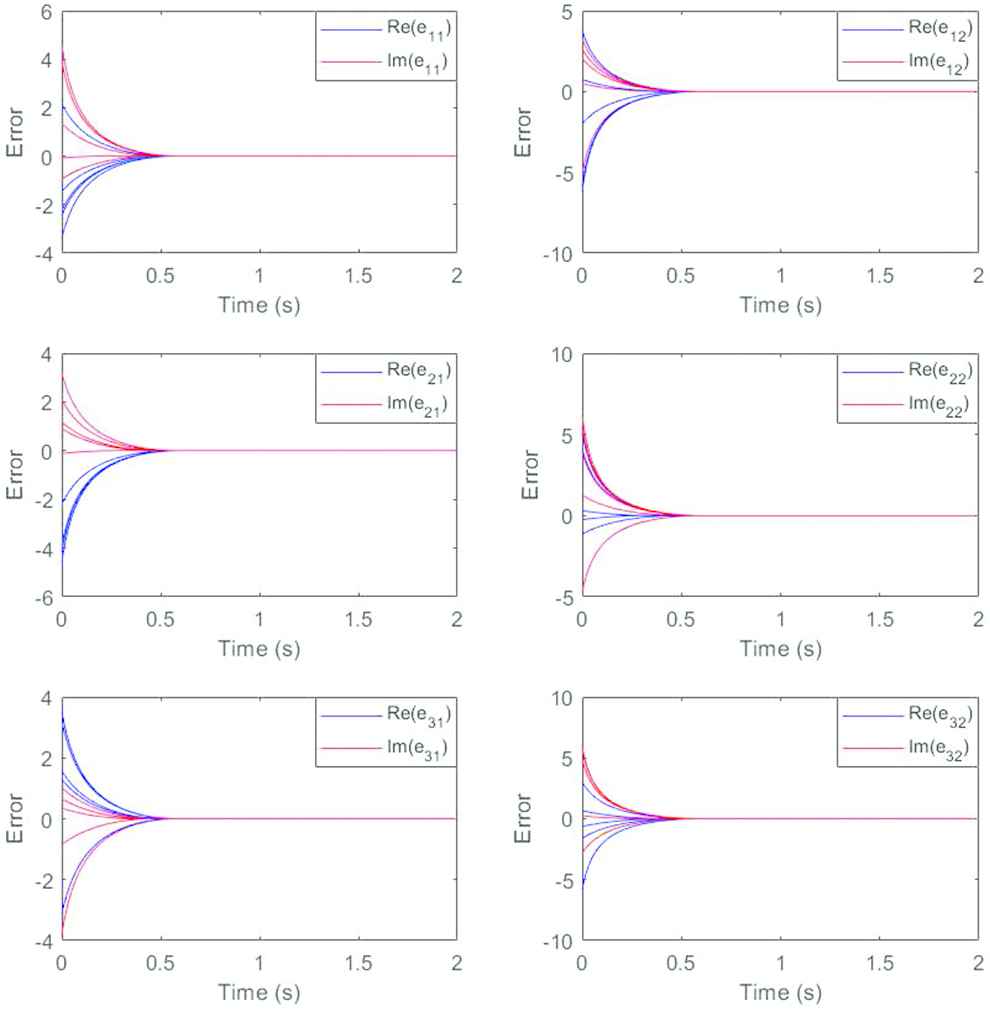
In order to further illustrate the validity of the conclusion, we plot the trajectory of the error function and the results are presented in Figure 2. We also divide the elements in the same position into real part and imaginary part and put them in the same diagram. It can be seen that starting from the same four initial values as before, the real part and imaginary part of each element rapidly converge to zero, indicating that the state solution can converge well to the theoretical solution. Compared with the traditional ZNN model proposed in another reference [30] that also solves the matrix Moore–Penrose inverse, the results in Figure 3 show that the variable parameter

Influence of parameters on convergence time for Example 1.
Example 2.
Consider the left Moore-Penrose inverse of the following complex time-varying matrix:
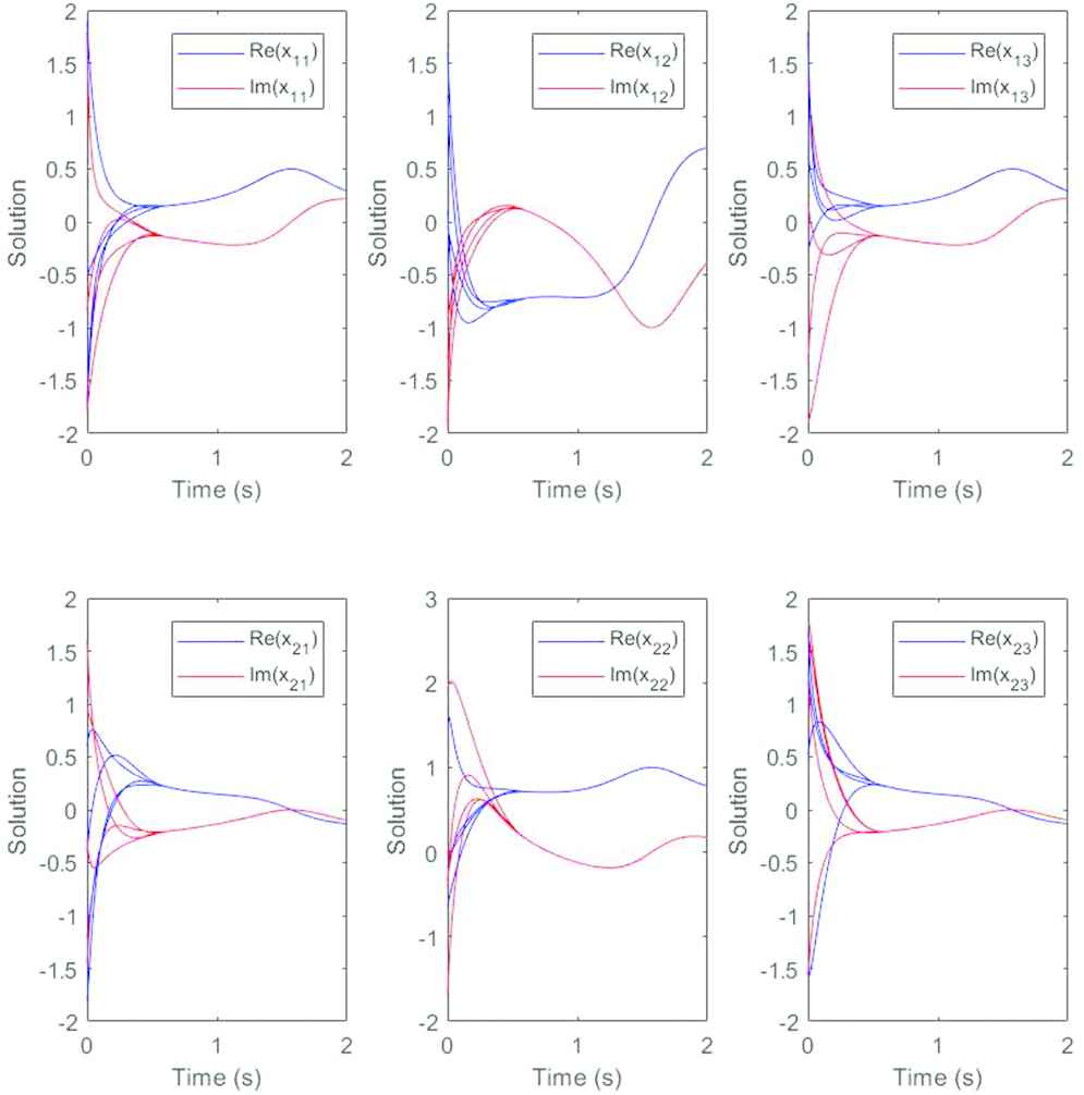
The ZNN model (12) is used to simulate the Moore–Penrose inverse of the time-varying matrix in Example 2. In this case, taking
Choosing four different initial values arbitrarily in every diagram, we divide the elements in the same position into real part and imaginary part. In order to reflect the convergence speed more intuitively, we put them in the same diagram. Similarly, as shown in Figures 4 and 5, we can observe that starting from any four given initial values, the solution curves of model (12) converges to one state corresponding to the elements of
Example 3.
Consider the right Moore–Penrose inverse of the following complex time-varying matrix with noise:
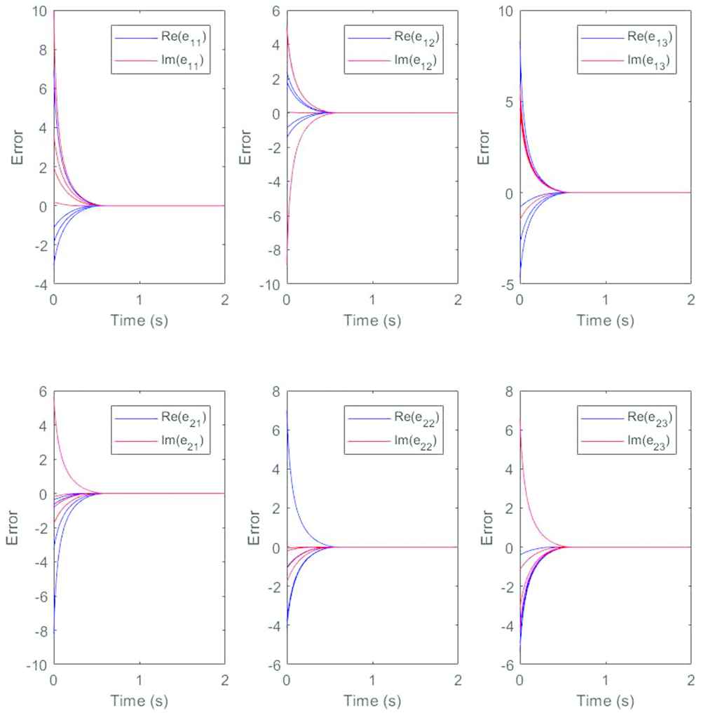
We first examine the stability of the model without interference from external noise. In order to further illustrate the validity of the conclusion, we plot the trajectory of the error function and it is shown in Figure 6. Obviously, every element in the error function, whether real or imaginary, will eventually converge to zero, which effectively proves that the model (14) can solve the time-varying Moore–Penrose inverse of matrices. Next, we randomly choose a set of constant noise values and compare the convergence of the error curves under this noise interference. It is clear that the error curves which are represented by the blue solid line and the blue dotted line in Figure 7 of model (14) both converges to zero faster. However, the error curves of model (7), which are the curves represented by red in Figure 7, converge slowly under the interference of external noise. In other words, model (14) does better in noise suppression.
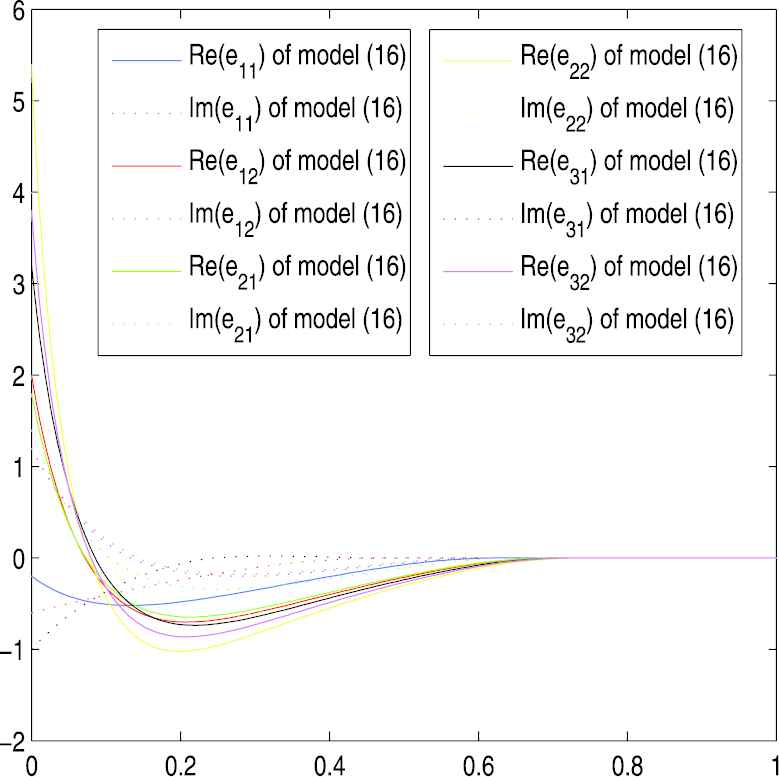
Trajectories of error function without noise for Example 3.
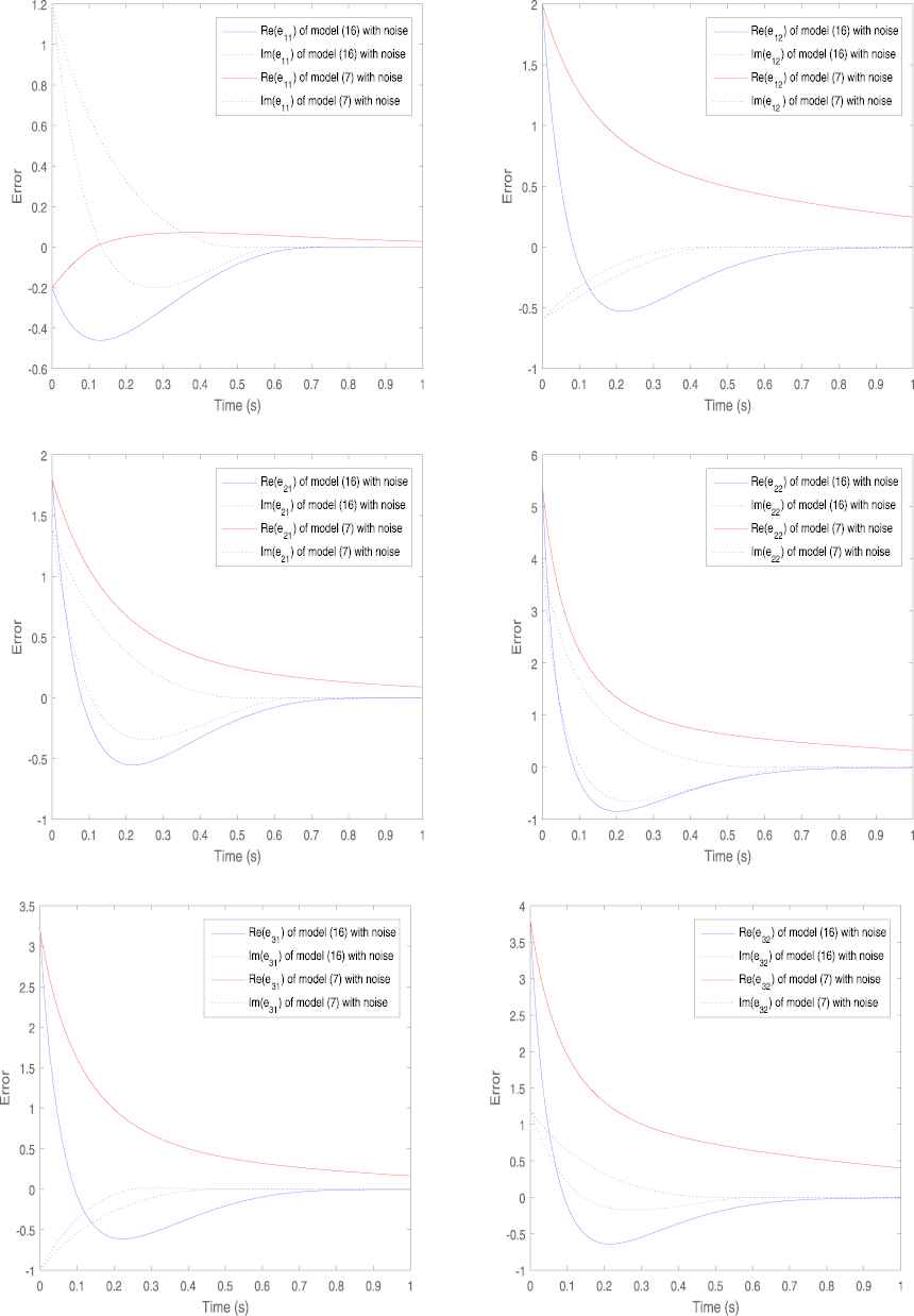
Trajectories of error function with noise for Example 3.
5. CONCLUSION
In this paper, for solving time-varying Moore–Penrose inverse over complex fields, a new ZNN model is proposed. The solution of the ZNN model (7) and the solution of the ZNN model (12) are proved to be stable in the sense of Lyapunov. Furthermore, for any initial value, the state solution of ZNN will converge to the theoretical solution in real time. Compared with existing results, our model converges faster because of the new activation function. The improved ZNN model (14) is proven to be more efficient in noise suppression. In addition, models with faster convergence rate and models for solving Moore–Penrose inverses of rank-deficient matrix would be one of our future research directions, which might achieve rich results under unremitting efforts.
CONFLICT OF INTEREST
The authors declare that we have no financial and personal relationships with other people or organizations that can inappropriately influence our work, there is no professional or other personal interest of any nature or kind in any product, service and/or company that could be construed as influencing the position presented in, or the review of, the manuscript entitled.
AUTHORS' CONTRIBUTIONS
Yiyuan Chai: Conceptualization and Methodology; Haojin Li: Writing- Original draft preparation; Defeng Qiao: Computer programs; Sitian Qin: Supervision, Validation and Investigation; Jiqiang Feng: Writing- Reviewing and Editing.
ACKNOWLEDGMENTS
This research is supported by the National Natural Science Foundation of China (61773136, 11871178).
REFERENCES
Cite this article
TY  - JOUR
AU  - Yiyuan Chai
AU  - Haojin Li
AU  - Defeng Qiao
AU  - Sitian Qin
AU  - Jiqiang Feng
PY  - 2020
DA  - 2020/06/17
TI  - A Neural Network for Moore–Penrose Inverse of Time-Varying Complex-Valued Matrices
JO  - International Journal of Computational Intelligence Systems
SP  - 663
EP  - 671
VL  - 13
IS  - 1
SN  - 1875-6883
UR  - https://doi.org/10.2991/ijcis.d.200527.001
DO  - 10.2991/ijcis.d.200527.001
ID  - Chai2020
ER  -