
Automatic Music Generator Using Recurrent Neural Network
 , Derwin Suhartono1
- DOI
- 10.2991/ijcis.d.200519.001How to use a DOI?
- Keywords
- Music generation; Music composition; Long short-term memory; Gated recurrent units; Subjective evaluation
- Abstract
In this paper, we developed an automatic music generator with midi as the input file. This study uses long short-term memory (LSTM) and gated recurrent units (GRUs) network to build the generator and evaluator model. First, a midi file is converted into a midi matrix in midi encoding process. Then, each midi is trained on a single layer and double stacked layer model of each network as a generator model. Next, classification model, based on LSTM and GRU, are trained and chosen as an objective evaluator to analyze the performance of each generator model which classify each midi based on its musical era. Subjective evaluation is conducted by an interview with volunteer respondents with various backgrounds such as classical music interest, performance, composer, and digital composer. The result shows that the double stacked layer GRU model perform better to resemble the composer pattern in music with 70% score of recall. Moreover, subjective evaluation shows that the generated music is listenable and interesting with the highest score of 6.85 out of 10 on double stacked layer GRU.
- Copyright
- © 2020 The Authors. Published by Atlantis Press SARL.
- Open Access
- This is an open access article distributed under the CC BY-NC 4.0 license (http://creativecommons.org/licenses/by-nc/4.0/).
1. INTRODUCTION
Music composition has been human's most popular hobby since long time ago. Recorded in the book “Ancient Greek Music: A Survey,” the oldest surviving complete musical composition is Seikilos Epitaph from 1st or 2nd century AD [1]. Algorithmic composition—composing by means of formalizable methods—Guido of Arezzo was the first inventing the music theory which mainly known as “solfeggio” in 1025. He invented a method to automate the conversion of text into melodic phrases [2]. Nowadays, the way of electronic instruments communicates with computer is through a protocol named music instrument digital interface (midi) which contains information such as pitch and duration [3]. Midi can be used for the composer to compose an orchestra without having the orchestra itself. Every part of the orchestra could be created from midi with synthesizer [4]. Digital audio workstation (DAW) is the standard in contemporary audio production which revolutionary capable in recording, editing, mastering, and mixing. DAW allows midi plays each channel separately into connected electronic devices or synthesizer [5]. The algorithmic composition has various approach such as Markov model, generative grammars, transition networks, artificial neural network, etc [2].
In his research, Weel [6] used Long Short-Term Memory (LSTM) method to train midi data and evaluate the output of music using subjective evaluation. He discovered that properly encoded midi could be used as an input for the recurrent neural network (RNN) and generate polyphonic music from any midi file, and network struggled to learn how to transition between musical structures. Nayebi et al. [7] compared LSTM and gated recurrent units (GRUs) method using wave file as its input with small size of datasets. They discovered that waveform input is possible with RNN and generating output of the LSTM networks was musically plausible. Kotecha et al. [8] used bi-axial LSTM trained with a kernel reminiscent of a convolutional kernel using the midi file as an input. They discovered that a two-layer LSTM model capable of learning melodic rhythmic probabilities from polyphonic midi files.
This study aims to compare the result of music generated with LSTM and GRU methods using midi as the input. Our main contribution is finding that the double stacked layer GRU model performs better like composer patterns and the generated music is pleasant to hear and interesting. The rest of the paper is organized as follows: Section 2 briefly reviews the literature of RNN. Section 3 describes the research method in detail. Result, and discussion are presented in Section 4. Finally, Section 5 gives the conclusion of this study.
2. RELATED WORKS
2.1. Recurrent Neural Networks
RNNs are in the family of feed-forward neural networks. They are different from other feed-forward networks in their ability to send information over time-steps [9]. RNN considering not an input x and an output y but a series (sequence) of inputs xt and outputs yt, indexed by a parameter t which represents the index or the time. The basic idea is that the outputs of a hidden layer (ht + 1) reenter into itself as an additional input to compute next values (ht + 1) of the hidden layer. This way, the network can learn, not only based on current data, but also on previous one. Therefore, it can learn series, notably temporal series [10]. Figure 1 shows that RNN can be viewed as many copies of a Feed Forward ANN executing in a chain.
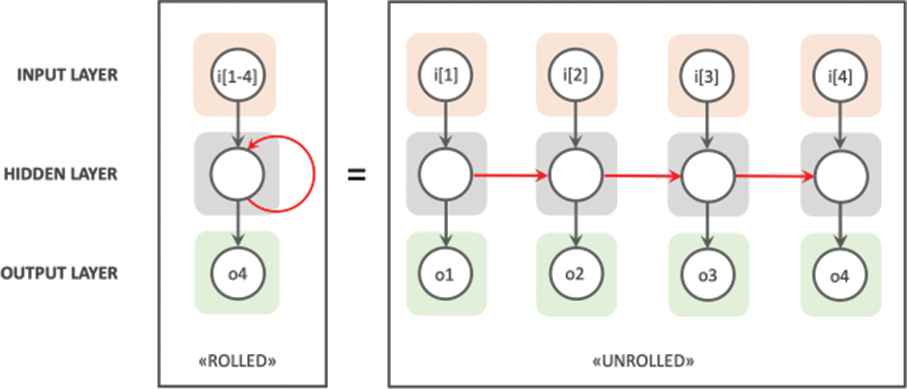
Recurrent neural networks (RNNs).
The recurrent networks suffered from a training problem caused by the difficulty to estimate gradients, because in backpropagation through time (BPTT), recurrence brings repetitive multiplications and could thus lead to over minimize or amplify effects called vanishing gradient problem [10]. BPTT is the back-propagation algorithm applied to the unrolled graph to estimate gradient of each step [11].
2.2. Long Short-Term Memory
LSTM unit was initially proposed by Hochreiter and Schmidhuber [12]. Since then, several minor modifications to the original LSTM unit have been made. We follow the implementation of LSTM as used in Greff [13].
A schematic of the LSTM block can be seen in Figure 2. It features three gates (input, forget, and output), block input, a single cell (the Constant Error Carousel), an output activation function, and peephole connections. The output of the block is recurrently connected back to the block input and all the gates [13].

Long short-term memory diagram.
2.3. Gated Recurrent Unit (GRU)
GRU was proposed by Cho et al. [14] to make each recurrent unit to adaptively capture dependencies of different time scales. Similarly, to the LSTM unit, the GRU, which can be seen in Figure 3, has gating units that modulate the flow of information inside the unit, however, without having a separate memory cell [15].
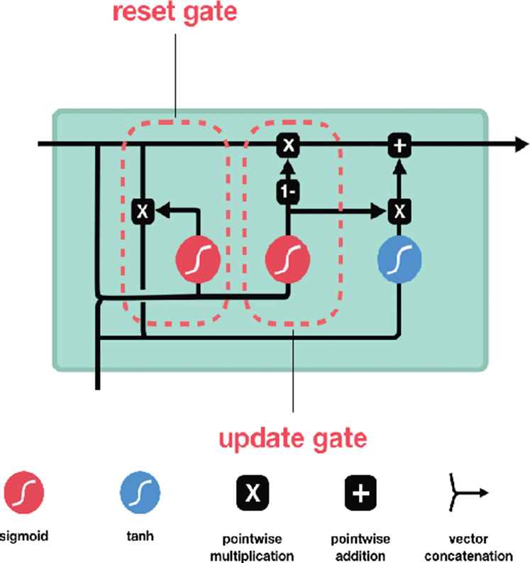
Gated recurrent unit.
3. PROPOSED METHODS
Methodology in this research is divided into several parts, such as midi collecting, midi encoding, music generation model training, generating music, music evaluation, and midi decoding.
3.1. Midi Collecting
67 midi files were downloaded from http://www.piano-midi.de and selected with multiple criteria. Midi must be in one of the classical eras, then it must be played with piano or keyboard. The time signature must be two or four quarter notes in a beat. The details of midi data per era shown in Table 1.
| Era | Amount of File |
|---|---|
| Baroque | 26 |
| Classical (Mozart only) | 12 |
| Romantic | 25 |
Midi classical data count.
As the number of midis are limited, each midi was transposed by 5 semitones up and down (Table 2) to increase the number of patterns input for the neural network.
| Era | Amount of File |
|---|---|
| Baroque | 26 |
| Classical (Mozart only) | 12 |
| Romantic | 25 |
Midi classical data count after transposed.
3.2. Midi Encoding
Midi file contains information of 128 pitch notes. Hence, there are only 88 pitch notes played in piano (A0–C8) from note number 21 till 108. Each of column in vector array sized 1 × 88 represents one pitch note of the piano. In quaver notes time signature, one vector array represents a sixteenth note (♫). In general, the midi encoding process can be seen in the flowchart in Figure 4. A midi file of music score shown in Figure 5.
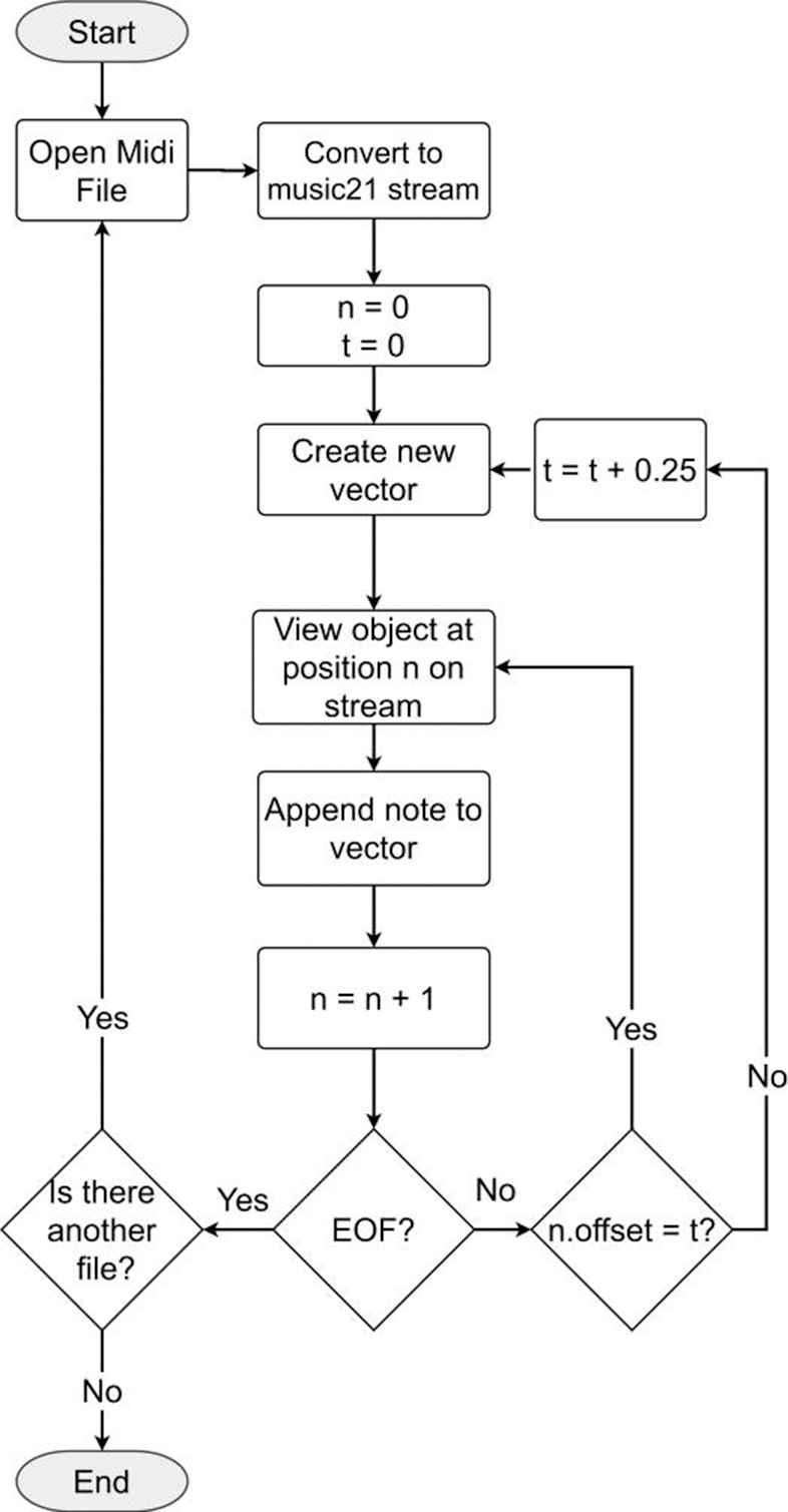
Midi encoding flowchart.
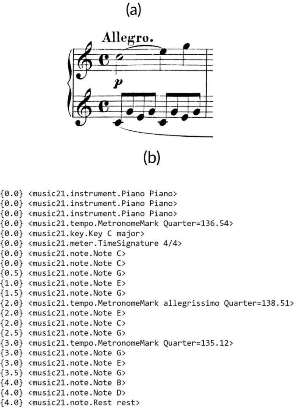
Mozart Piano Sonata no. 16. (a) First bar in music score. (b) First bar in music21 stream object.
(a) converted into a flat-midi stream which will flatten midi into a single channel using music21 (shown in Figure 5(b)). Music21 stream object is the container of offset-positioned notation and music elements in music21. One event of a stream is noted as n and the time it performs in called offset t. For instance, the first row of the stream shown in Figure 5(b) n = 0, offset t = 0.0 with information played with piano. As one midi event n only contain one information, then the information on one offset t written in several event.
One array vector sized 1 × 88 represents 0.25 value of offset. Therefore, one beat of quaver note is composed of 4 array vectors (shown in Figure 6).
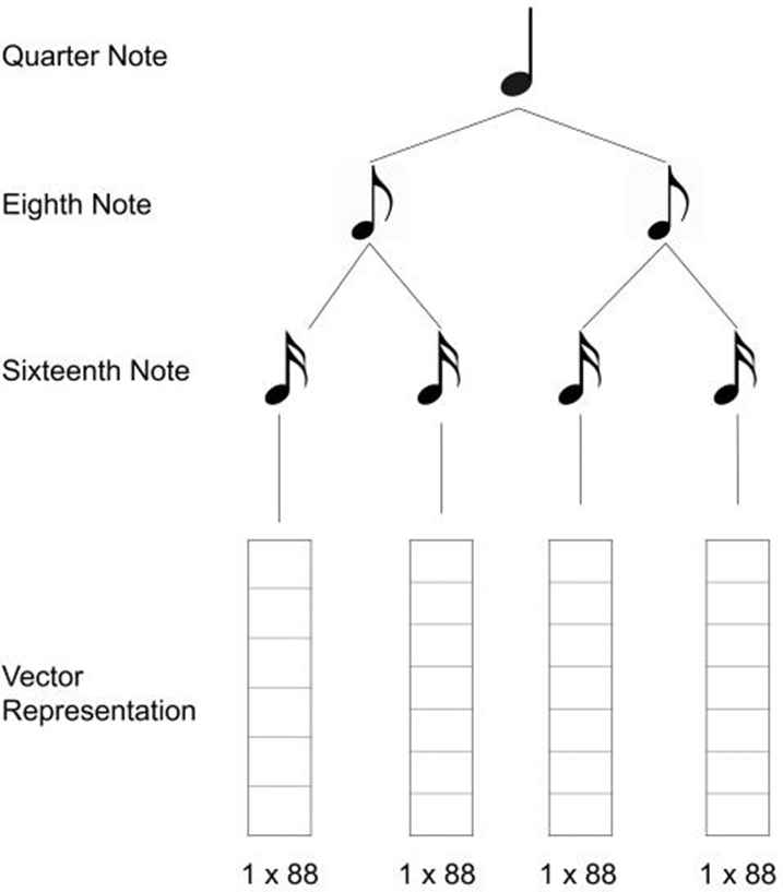
Vector representation of a quaver note.
The result of the midi encoding process is one 88 × t matrix table. Its column indicates the time and 88 rows corresponding to the pitch which each cell contains a note velocity. Midi of one bar Piano Sonata No. 16 can be represented visually in midi editor shown in Figure 7(a). In Midi Editor, each row on represents a pitch note and executed note is defined with a rectangle which its width represents duration of and the result of midi encoding process is shown in Figure 7(b).

Representation of one bar of Mozart Piano Sonata No. 16 midi. (a) Visual representation. (b) Matrix representation.
3.3. Music Generation Model Training
The midi matrix generated from midi encoding process is distributed into some set of sequence input and output (interpret visually in Figure 8). With sequence length 16, the first 16 data from the midi matrix become sequence input (red box) and the vector after it became the sequence output (blue box). Then the window will slide by one till the end of matrix.

Visualization of input and output on Midi Matrix. Red box represents the sequence input and blue box represents the sequence output.
In conducting the training process, the optimizer used is RMSprop with learning rate η = 0.001. Since the model trained is a regression model, the loss function selected is mean squared error (MSE) with epoch 64 and batch_size 32. Small batch_size is chosen to prevent memory used does not exceed the available memory.
The models to be built are single layer LSTM, single layer GRU, double stacked layer LSTM, double stacked layer GRU. The components in each model are as follows:
Components for single layer LSTM model as put in Figure 9 are
Input size is 1 × sequence length × 88
One-layer LSTM with 512 nodes
Dense 88 nodes with linear activation function which connected to the output
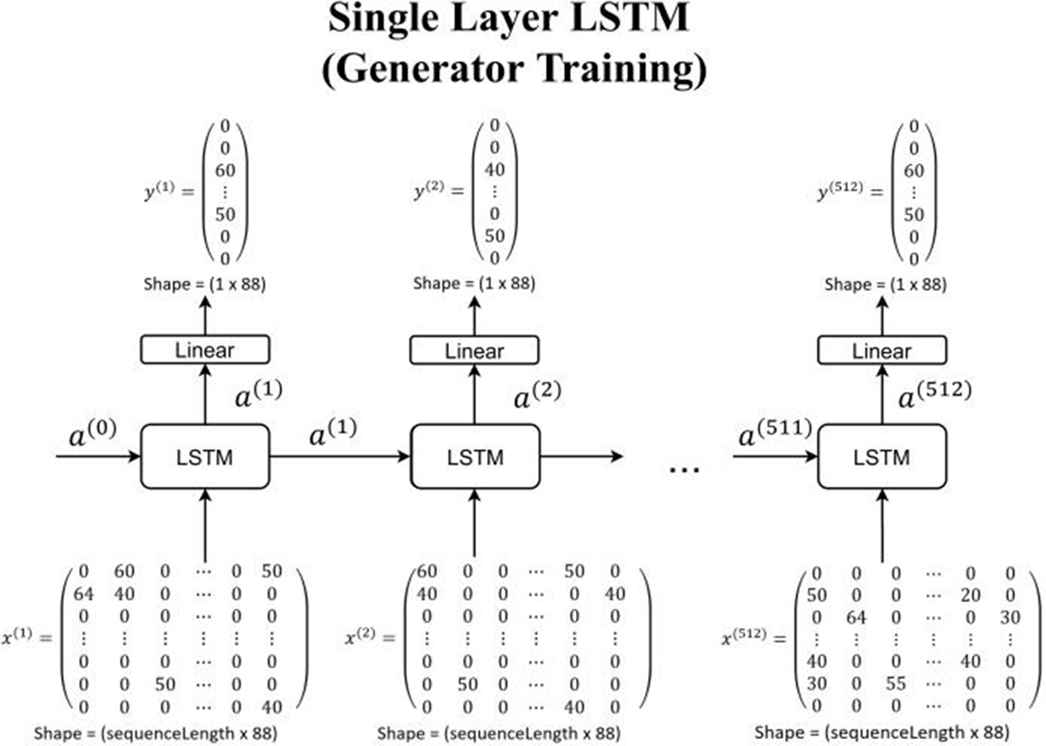
Single layer long short-term memory (LSTM) model for generator training.
Components for single layer GRU model as put in Figure 10 are
Input size is 1 × sequence length × 88
One-layer GRU with 512 nodes
Dense 88 nodes with linear activation function which connected to the output
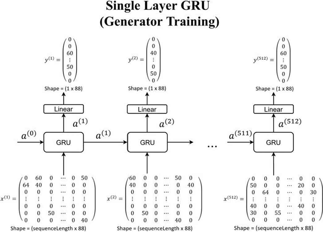
Single layer GRU model for generator training.
Components for double stacked layer LSTM model as put in Figure 11 are
Input size is 1 × sequence length × 88
One-layer LSTM with 512 nodes
Dropout 0.1
One-layer LSTM with 512 nodes
Dense 88 nodes with linear activation function which connected to the output
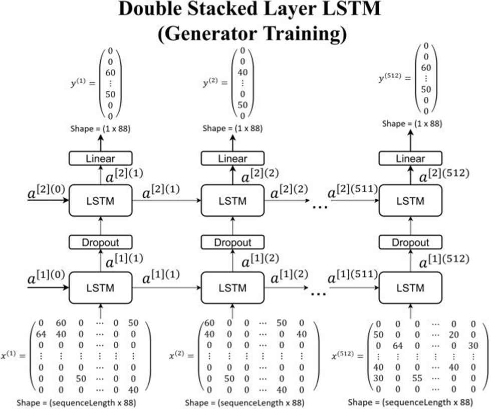
Double stacked layer long short-term memory (LSTM) model for generator training.
Components for double stacked layer GRU model as put in Figure 12 are
Input size is 1 × sequence length × 88
One-layer GRU with 512 nodes
Dropout 0.1
One-layer GRU with 512 nodes
Dense 88 nodes with linear activation function which connected to the output
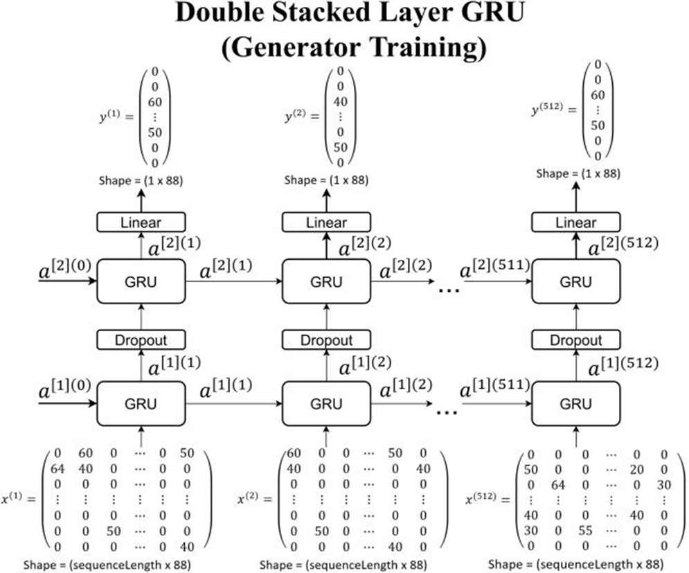
Double stacked layer gated recurrent unit (GRU) model for generator training.
3.4. Music Generation Model Training
In this step, model trained from music generator used to generate the music from the input given.
Assume that the sequence length of trained model was 16, then the generating process is shown in Figure 13. The sequence input in Figure 13(a) from vector 0–15 inserted into the model to generate a 1 × 88 array vector as the next vector. Then the generated vector will be appended to the input as vector 16. Then the sequence input is sliding so the vector 1–16 inserted into the model and generate a new vector (shown in Figure 13(b)). This step is looping until 512 new vectors generated. The music is used for the evaluation in the next process.
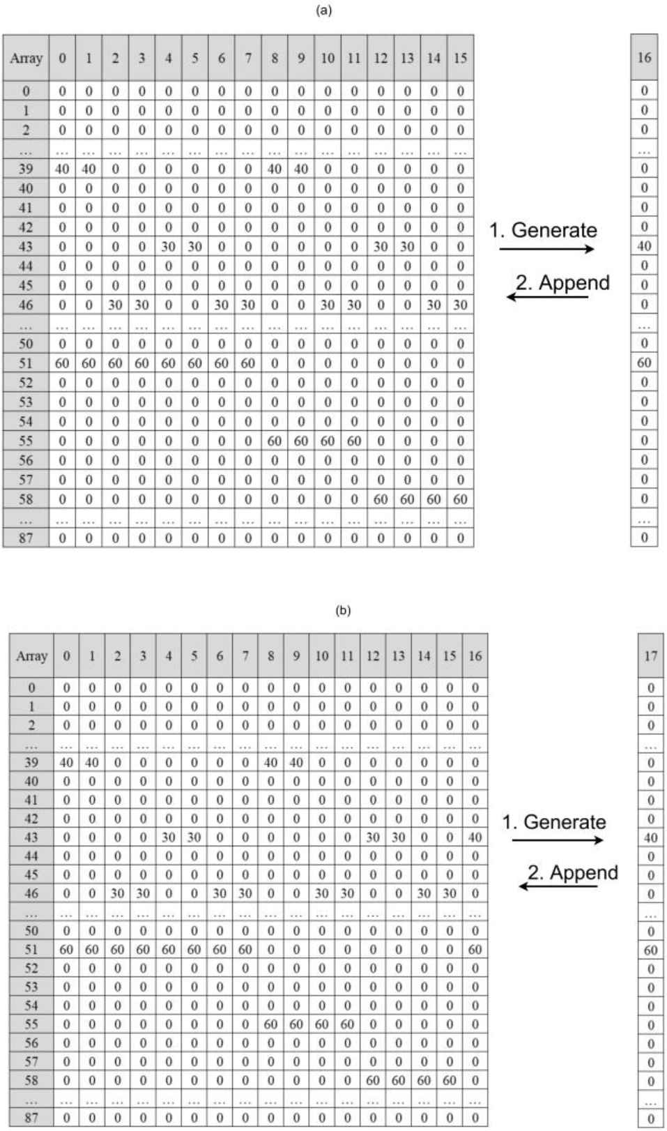
Generating process visualization. (a) First generating process. (b) Second generating process.
3.5. Music Evaluation
Each midi was classified based on its era before the evaluator training process. If it is classical it will be label as 1, otherwise 0. The encoded midi from midi encoding process normalized so that it values are in range 0–1.
In conducting the training process, the optimizer used is RMSprop with learning rate η = 0.001. Since the model trained is a classification model, the loss function selected is binary cross-entropy with epoch 64 and batch_size 32.
The classification model to be built are double stacked layer LSTM and double stacked layer GRU. The components in each model are as follows:
Components for LSTM evaluator model as put in Figure 14 are
Input size is 1 × 1845 × 88
One-layer LSTM with 64 nodes
Dropout 0.5
One-layer LSTM with 64 nodes
Given output layer with sigmoid activation function on the last node which connected to the output
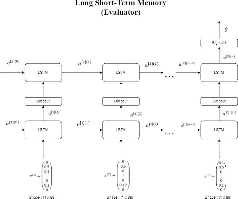
Long short-term memory (LSTM) evaluator model.
Components for GRU evaluator model as put in Figure 15 are
Input size is 1 × 1845 × 88
One-layer GRU with 64 nodes
Dropout 0.5
One-layer GRU with 64 nodes
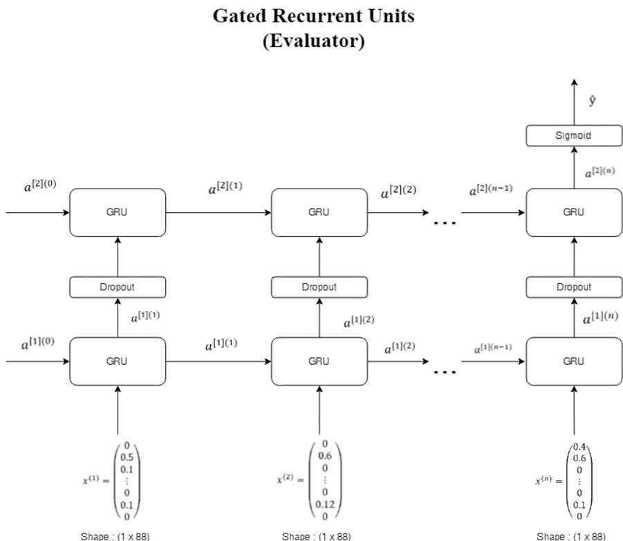
Gated recurrent unit (GRU) evaluator model.
Given output layer with sigmoid activation function on the last node which connected to the output.
3.6. Music Decoding
Midi matrix from music generating process has a size of 272×88 which each vector represents one semiquaver notes with a total of 272 vectors. To decode the midi matrix back to midi files, each vector will be written into stream object. This process can be seen in Figure 16. Since the dimension of the midi matrix is a two-dimensional array, then it will be iterated in x and y. If the note velocity is not zero, then the note velocity on the cell (x, y) will be written into note object and appended into the stream object. Every note object is formed in the following form: (offset, note, velocity, duration).
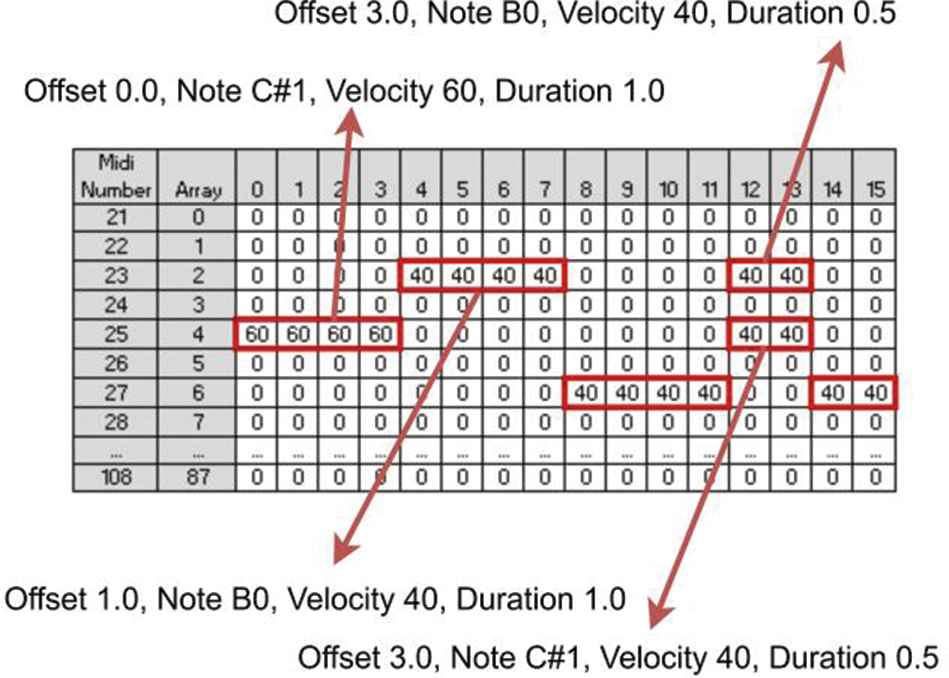
Decoding example of midi matrix.
4. RESULTS AND ANALYSIS
4.1. System Specification and Datasets
The training was run using Google Datalab platform with specification as described in Table 3.
| Hardware | Specification |
|---|---|
| Processor | 8 v CPUs of Intel Xeon E5 v2 @2.5 GHz |
| Memory | 52 GB |
| Hard disk drive | 200 GB |
| Graphics card | 16 GB Nvidia Tesla K80 |
| Operating system | Debian Linux 9 |
| Platform | Google Datalab |
Specifications of Google Datalab platform.
The midi file gathered from the midi collecting process was arranged into two datasets as explained in Table 4.
| Dataset Name | Midi Files | Description |
|---|---|---|
| dsGenerator | 12 | 12 midi files in classical era |
| dsEvaluator | 693 | 132 midi files classical era and 561 midi files nonclassical era |
List of datasets.
4.2. System Specification and Datasets
In this subsection, the model trained will be analyzed in a group of two experiments. The training process used dsGenerator dataset which contains 12 midi files, encoded into 38,141 array vectors and converted with sequence length 16 into 38,125 sets of sequences. The sequence separated into training and validation data with a ratio of 9:1 and became the input of each model.
The first experiment was conducted on single layer LSTM and single layer GRU model. Last trained data was run on January 26th, 2019 and took approximately 2 hours on single layer LSTM and 1 hour on single layer GRU.
Figure 17 showed that the accuracy of both models was tended to increase without any drop drastically in each epoch. Therefore, both models succeeded to learn the data input with the following accuracy as depicted in Table 5.
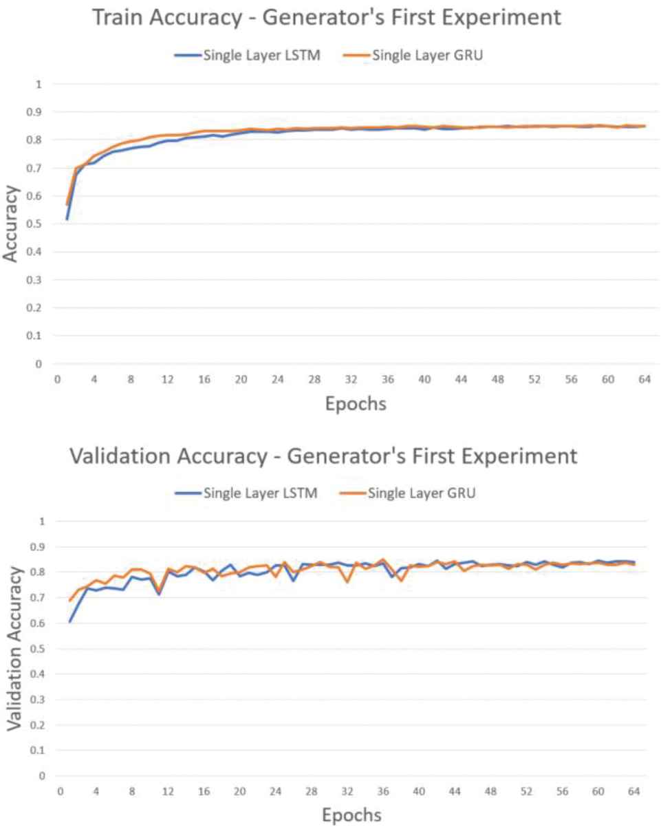
Accuracy graph of experiment with single layer recurrent neural network (RNN).
| Method | Training Accuracy | Validation Accuracy |
|---|---|---|
| LSTM | 0.8501 | 0.8399 |
| GRU | 0.8498 | 0.8278 |
RNN, recurrrent neural network; LSTM, long short-term memory; GRU, gated recurrent unit.
Generator accuracy on single layer RNN.
The second experiment was conducted on double stacked layer LSTM and double stacked layer GRU model. Last trained data was run on January 26th, 2019 and took approximately 3 hours on double stacked layer LSTM and 1.5 hours on double stacked layer GRU.
Figure 18 showed that the accuracy of both models was tended to increase without any drop drastically in each epoch. It showed that each model succeeded to learn the data input. However, the second experiment is more stable and achieves higher accuracy than the first experiment on each epoch with the accuracy as illustrated in Table 6.
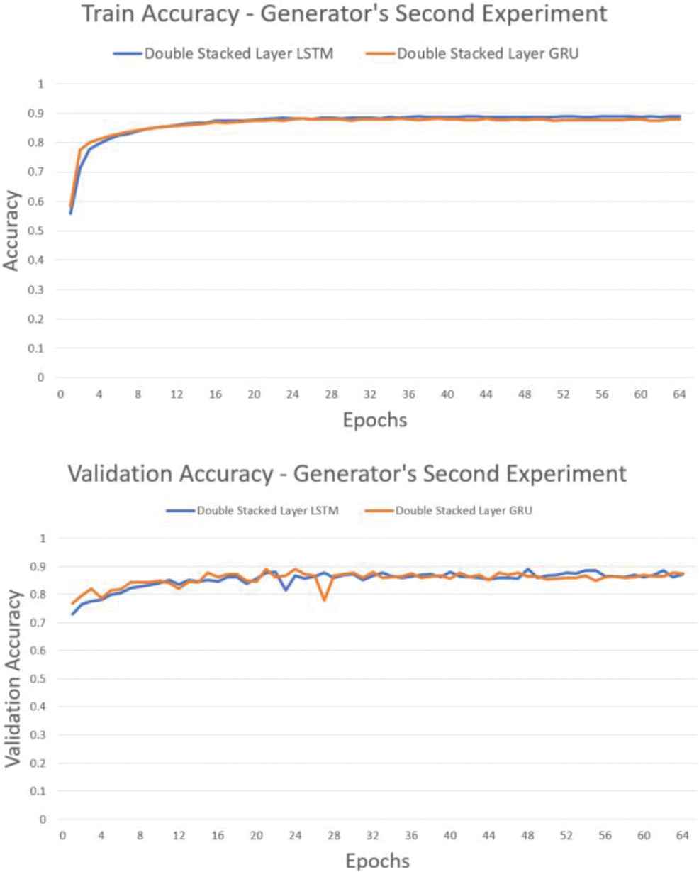
Accuracy graph of experiment with double stacked recurrent neural network (RNN).
| Method | Training Accuracy | Validation Accuracy |
|---|---|---|
| LSTM | 0.8887 | 0.8721 |
| GRU | 0.8781 | 0.8735 |
RNN, recurrrent neural network; LSTM, long short-term memory; GRU, gated recurrent unit.
Generator accuracy on double stacked layer RNN.
Then both experiments model evaluated objectively using evaluator model and subjectively using user scoring.
4.3. Evaluator Model Analysis
In this subsection, the evaluator model trained using dsEvaluator dataset which contains a total of 673 files. The dataset separated into training, validating, and testing data with a ratio of 8:1:1 and became the input of each model using batch size 32. Last trained data was run on January 28th, 2019 and took approximately 8 hours on LSTM model and 6 hours on GRU model.
Figure 19 showed that the accuracy of LSTM dropped drastically in epoch 32. It tells that the LSTM evaluator model tends to overfit. However, GRU model tended to increase in each epoch with the following accuracy:
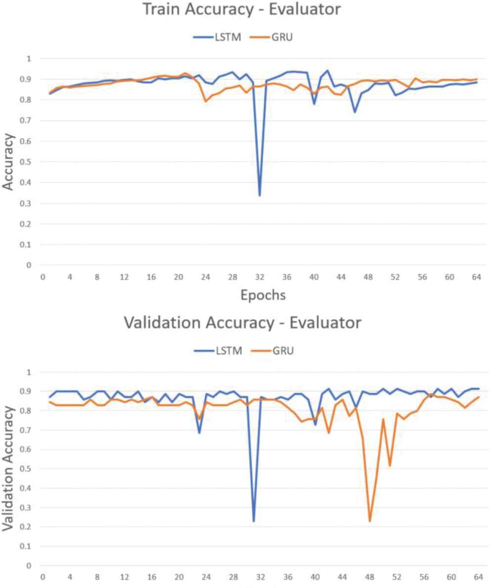
Accuracy graph of evaluator.
Each training and validation accuracy of evaluator showed in Table 7. It was clear that the LSTM has failed to learn the data input hence has a lower training accuracy than the validation.
| Method | Training Accuracy | Validation Accuracy |
|---|---|---|
| LSTM | 0.8831 | 0.9143 |
| GRU | 0.8993 | 0.8714 |
LSTM, long short-term memory; GRU, gated recurrent unit.
Accuracy on evaluator.
Furthermore, to measure the performance of each classification model, a classification comparison was carried out which compare the system output and its actual label to obtain the value of true positive (tp), true negative (tn), false positive (fp), false negative (fn).
With the information shown in Tables 8 and 9. Recall value calculated from the number of true positive over sum of true positive and false negative. Thus, LSTM model achieve 15% of recall and GRU model achieve 20% of recall. Therefore, GRU model was chosen to evaluate the generator model.
| Predicted |
|||
|---|---|---|---|
| True | False | ||
| Actual | True | 3 | 17 |
| False | 0 | 47 | |
LSTM, long short-term memory.
Confusion matrix of LSTM model.
| Predicted |
|||
|---|---|---|---|
| True | False | ||
| Actual | True | 4 | 16 |
| False | 2 | 45 | |
GRU, gated recurrent unit.
Confusion matrix of GRU model.
4.4. Objective Evaluation
Objective evaluation was conducted by looking at the recall value of each experiment using evaluator model. 20 midi files were generated toward each model and became the input of evaluator model to classify whether its classical or nonclassical. The details were shown in the following Table 10.
| Experiment | Recall Value |
|
|---|---|---|
| LSTM | GRU | |
| Experiment 1 (single layer) | 0.0 | 0.0 |
| Experiment 2 (double stacked layer) | 0.3 | 0.7 |
LSTM, long short-term memory; GRU, gated recurrent unit.
Recall value of experiments.
From both experiments, double stacked layer GRU model performs better than another model with a recall of 70%. However, we could not conclude which method performs better, further research in music generation with massive data is required.
4.5. Subjective Evaluation
Subjective evaluation was directed by an interview with 10 volunteer respondents to evaluate the music generated from each model. Respondent of this interview was the audience with classical music interest, performer, composer, and digital composer. Each respondent was given a short explanation of automatic music generator application and chance to using the application.
Two midi files were generated randomly from http://tones.wolfram.com with multiple criteria, the music style must be piano, with tempo is four notes per beats. Then they were become an input of each model. The respondent listened to 8 music which generated by using 2 inputs and 4 models whose arrangement had been randomized. The details of music are shown in Tables 11 and 12. The results of subjective evaluation can be seen in Table 12 and Table 13.
| Song Title | Music Input Title | Model |
|---|---|---|
| Song-1 | Song-A | Double stacked layer LSTM |
| Song-2 | Song-B | Single layer GRU |
| Song-3 | Song-B | Single layer LSTM |
| Song-4 | Song-A | Single layer LSTM |
| Song-5 | Song-A | Double stacked layer GRU |
| Song-6 | Song-A | Single layer GRU |
| Song-7 | Song-B | Double stacked layer GRU |
| Song-8 | Song-B | Double stacked layer LSTM |
LSTM, long short-term memory; GRU, gated recurrent unit.
Arrangement of generated music.
| Single Layer LSTM |
Single Layer GRU |
|||||
|---|---|---|---|---|---|---|
| Song A | Song B | Average | Song A | Song B | Average | |
| Respondent 1 | 3 | 3 | 3 | 2.5 | 2.5 | 2.5 |
| Respondent 2 | 1 | 1 | 1 | 1 | 1 | 1 |
| Respondent 3 | 5 | 4 | 4.5 | 4 | 3 | 3.5 |
| Respondent 4 | 1 | 4 | 2.5 | 1 | 2 | 1.5 |
| Respondent 5 | 6 | 4 | 5 | 5 | 4 | 4.5 |
| Respondent 6 | 4 | 5 | 4.5 | 3 | 4 | 3.5 |
| Respondent 7 | 3 | 3 | 3 | 4 | 5 | 4.5 |
| Respondent 8 | 7 | 7 | 7 | 6.5 | 7.5 | 7 |
| Respondent 9 | 3 | 2 | 2.5 | 1 | 3 | 2 |
| Respondent 10 | 3 | 4 | 3.5 | 2 | 2 | 2 |
| Average Score | 3.65 | 3.2 | ||||
RNN, recurrrent neural network; LSTM, long short-term memory; GRU, gated recurrent unit.
Score of music from each respondent (single layer RNN).
| Double Stacked Layer LSTM |
Double Stacked Layer GRU |
|||||
|---|---|---|---|---|---|---|
| Song A | Song B | Average | Song A | Song B | Average | |
| Respondent 1 | 5 | 7 | 6 | 7 | 8.5 | 7.75 |
| Respondent 2 | 2 | 2 | 2 | 2 | 2 | 2 |
| Respondent 3 | 8 | 6 | 7 | 5 | 8 | 6.5 |
| Respondent 4 | 7 | 7 | 7 | 8 | 7 | 7.5 |
| Respondent 5 | 8 | 7.5 | 7.75 | 7 | 7.5 | 7.25 |
| Respondent 6 | 7 | 6 | 6.5 | 9 | 8 | 8.5 |
| Respondent 7 | 5 | 3 | 4 | 8 | 8 | 8 |
| Respondent 8 | 8 | 7.5 | 7.75 | 8 | 8 | 8 |
| Respondent 9 | 8 | 5 | 6.5 | 7 | 6 | 6.5 |
| Respondent 10 | 4 | 5 | 4.5 | 6 | 7 | 6.5 |
| Average Score | 5.9 | 6.85 | ||||
RNN, recurrrent neural network; LSTM, long short-term memory; GRU, gated recurrent unit.
Score of music from each respondent (double stacked layer RNN).
Each music generated will be played to the respondent, a score was given in range of 1–10 which score 1 is the lowest score and score 10 is the highest score and wrote their opinion or review of the music.
The main point from each interview was summarized in the following list:
The music generated from double stacked layer GRU is a music with score 6.85 out of 10
The music is interesting and acceptable but need more improvement
Some respondent said that articulation, dynamics, chord progression, musical phrasing, and sustained pedal must be considered to create a music. However, automatic music generator could not completely substitute the human needs such as human touch and tone color.
5. CONCLUSIONS AND FUTURE WORKS
From the experiments, evaluation, and interviews, double stacked layer GRU model can perform better to resemble the composer pattern in music with 70% score of recall. Classification model could be used to classify the generator model using double stacked layer GRU with an accuracy of 89.93%. The music generated was listenable and interesting which the highest score is double stacked layer GRU model with a score of 6.85 out of 10. In future research, the dynamics tempo with larger datasets can be considered in the midi encoding process as new information to the neural networks. As the sequence length means the length of sequence input in model, additional sequence length can be considered to enhance the model output.
CONFLICT OF INTEREST
The authors declare that they have no competing interests.
AUTHORS' CONTRIBUTIONS
The study was conceived and designed by Alexander Agung Santoso Gunawan. The experiments are performed by Ananda Phan Iman. The writing is conducted by Derwin Suhartono and Ananda Phan Iman. All authors read and approved the manuscript.
ACKNOWLEDGMENTS
This work is supported by Bina Nusantara University, as a part of Publikasi Unggulan BINUS 2020. The authors would like to thank the referees.
REFERENCES
Cite this article
TY  - JOUR
AU  - Alexander Agung Santoso Gunawan
AU  - Ananda Phan Iman
AU  - Derwin Suhartono
PY  - 2020
DA  - 2020/06/25
TI  - Automatic Music Generator Using Recurrent Neural Network
JO  - International Journal of Computational Intelligence Systems
SP  - 645
EP  - 654
VL  - 13
IS  - 1
SN  - 1875-6883
UR  - https://doi.org/10.2991/ijcis.d.200519.001
DO  - 10.2991/ijcis.d.200519.001
ID  - Gunawan2020
ER  -