
An Improved Parameter Control Based on a Fuzzy System for Gravitational Search Algorithm
- DOI
- 10.2991/ijcis.d.200615.001How to use a DOI?
- Keywords
- Gravitational search algorithm; Fuzzy system; Fuzzy rules; Optimization
- Abstract
Recently, a kind of heuristic optimization algorithm named gravitational search algorithm (GSA) has been rapidly developed. In GSA, there are two main parameters that control the search process, namely, the number of applied agents (Kbest) and the gravity constant (G). To balance exploration and exploitation, a fuzzy system containing twelve fuzzy rules is proposed to intelligently control the parameter setting of the GSA. The proposed method can enhance the convergence ability and yield better optimization results. The performance of fuzzy GSA (FGSA) is examined by fifteen benchmark functions. Extensive experimental results are tested and compared with those of the original GSA, CGSA, CLPSO, NFGSA, PSGSA and EKRGSA.
- Copyright
- © 2020 The Authors. Published by Atlantis Press SARL.
- Open Access
- This is an open access article distributed under the CC BY-NC 4.0 license (http://creativecommons.org/licenses/by-nc/4.0/).
1. INTRODUCTION
As optimization problems have become increasingly complicated, the traditional methods cannot effectively solve them in a high-dimensional search space. Hence, heuristic search algorithms have come into being. Heuristic optimization methods are developed based on natural or physical processes. Algorithms inspired by the behavior of natural phenomena have received widespread attention over the past few decades [1–4].
The superior performance of gravitational search algorithm (GSA) has attracted increasing attention. In recent years, many modified versions of GSA have been proposed. The most famous are the real GSA [5], introduced for real-valued variables; the binary GSA [6], which has variables with a value of either 0 or 1; the discrete GSA [7], possessing variables with discrete values; and the mixed GSA [8], containing both continuous and binary variables.
To control exploitation and exploration efficiently, some new GSA operators have been designed, including disruption [9–11], chaotic [12,13], mutation [14], crossover [15], and so on.
In the original GSA, the parameters mainly consist of the following aspects: mass of agent (M), number of agents (N), gravitational constant (G), distance between agents in the search space (R), power between distances (P) and number of applied agents (Kbest). The number of agents is generally set at the beginning of the algorithm and fixed during operation [16]. M has three attributes [5]: active gravitational mass, which determines the intensity of the gravitational field produced by an agent; passive gravitational mass, which determines the strength of an agent's interaction with the gravitational field and inertial mass, which represents the intensity of resistance to motion change when a force acts on an agent. The value of N is set according to the requirements of the specific algorithm used. The distance between agents is calculated as a function of the Euclidian distance, and the power between distances is set to one in the GSA and all its variants.
The values of the masses in the original GSA, including the passive mass, active mass and inertia mass, are set to the same value. Javidi suggested that mass calculation should be improved by defining an opportune function named sigma scaling and the Boltzmann functions [17]. These functions try to balance exploration and exploitation to prevent the algorithm from falling into local optimum. Khajooei and Rashedi proposed a function related to the concept of antigravity, which utilizes both positive and negative masses. The algorithm aims to enhance the ability to explore the search space [18].
In most GSA versions, both G and Kbest follow the same rules and decrease as the number of iterations increases [19]. In the original GSA, Kbest is obtained by the decreasing function in Eq. (1) [5]:
The NFGSA [21] proposed a neural network combined with a fuzzy system to adjust the parameter
In the binary GSA,
Fatemeh and Esmat use a fuzzy rule for controlling GSA setting [22]. In their opinion, the distance between agents (
In another study [23], the authors deemed that the value of
According to the two parameter control methods based on fuzzy theory mentioned above, the former uses two functions to control two input parameters, which represent the population diversity and population progress respectively. However, although these fuzzy rules of the former are used to control the parameter
It is important to control exploitation and exploration in GSA. A new fuzzy system is applied to intelligently control the parameters of GSA, which includes twelve fuzzy rules. They are adopted to increase the convergence rate and prevent the algorithm from falling into local optimum.
New control functions are designed to calculate the value of the input variables so that the agent diversity and optimization progress of GSA can be well monitored.
Compared with the original GSA, CGSA, CLPSO, NFGSA, PSGSA and EKRGSA, the proposed method has achieved better results for fifteen well-known standard functions. Additional experiments have indicated that these fuzzy rules are effective.
This paper consists of five sections. Introduction is firstly suggested as Section 1. After that, GSA is reviewed in Section 2. In Section 3 fuzzy GSA is described in detail. Experimental results are presented in Section 4. At last, conclusions are included in Section 5.
2. GRAVITATIONAL SEARCH ALGORITHM
In GSA, the objective function of an optimization problem is based on many variables. Each variable has an upper and a lower bound, as shown in Eq. (7), represented by
Let
Then, the law of motion is used to calculate the acceleration of the agents, as shown in Eq. (10):
The gravitational constant
The masses of the agents are calculated by the fitness evaluation. Supposing that the gravitational mass is numerically equal to the inertia mass, the mass
To control important parameters, the original GSA uses a mathematical model, which includes linearity, an exponential character or both. As the iteration proceeds, the exploration becomes weaker and the exploitation becomes stronger. However, when faced with complex engineering problems, such as big data analysis, the problem becomes nonlinear and complex. It is not enough to control the algorithm process through a mathematical model [23]. An effective solution is to establish a balance between exploration and exploitation through parameter control.
3. FUZZY GSA
Currently, many scholars combine heuristics methods with fuzzy logic to improve algorithms [22,24–26]. They integrate algorithm processes with the linguistic description to create a fuzzy system to intelligently control parameters. In GSA, the larger the agent is, the slower the convergence rate is and the better the diversity is; the smaller the agent is, the easier it is for the agent to fall into the local optimum.
In the original GSA, there are two important parameters, i.e.,
3.1. Kbest and G
The parameter
3.2. Agent Diversity and Optimization Progress
Agent diversity and optimization progress are the most effective tools for monitoring the performance of the algorithm [22]. The parameter
The positions of the agents in the search space are not far apart. In this case, the objective function has fallen into the local optimum at similar locations in the search space.
The positions of the agents in the search space are far apart. In this case, the objective function has at least 2 local optima at different locations in the search space.
Both conditions indicate that the objective function is trapped in the local optimum regardless of whether the locations of the agents are similar or different, which implies that the diversity of the agents is poor, and vice versa.
In addition to
The smaller
3.3. Membership Functions
A fuzzy inference system is composed of three input variables and two output variables.
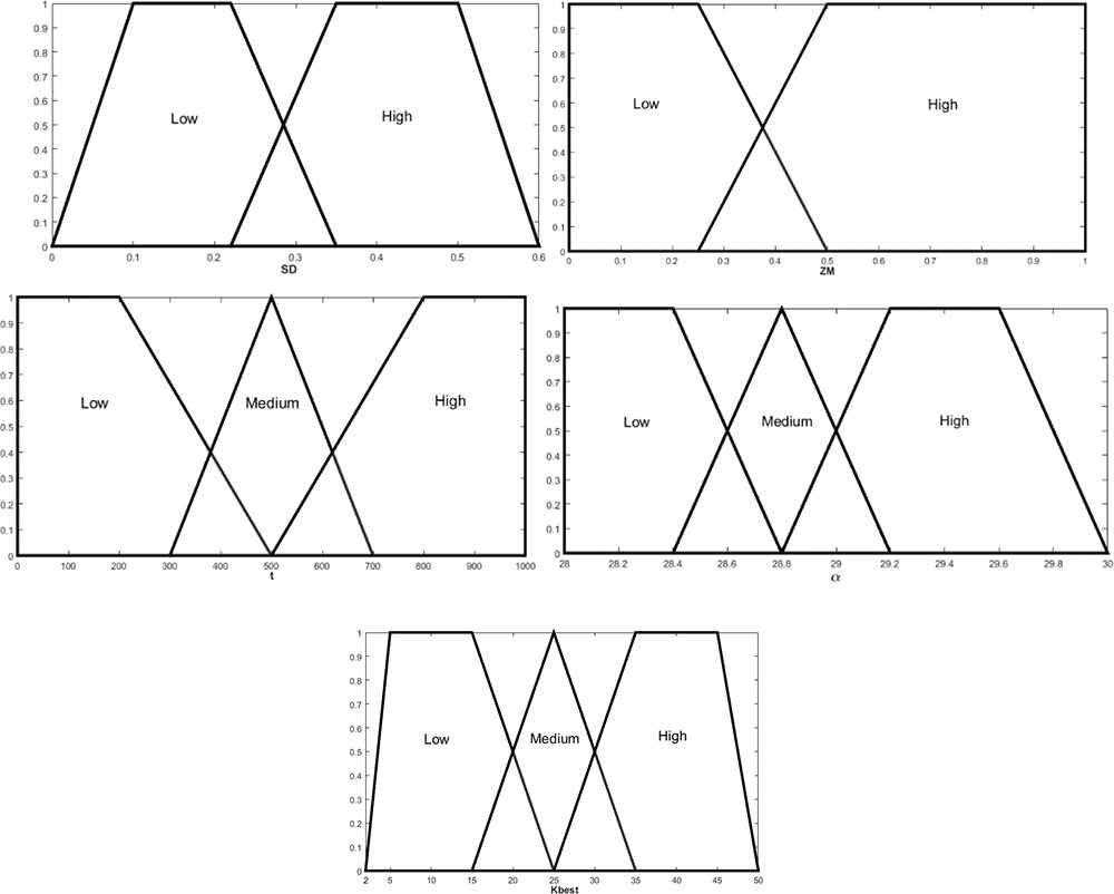
Membership functions.
3.4. Fuzzy Rules
Twelve fuzzy rules are extracted from the previous subsections with three input and two output variables, as shown in Table 1. These rules are proposed to intelligently control the search process of GSA, prevent the algorithm from falling into a local optimum and avoid premature convergence. Each of the fuzzy rules is set up to enhance the performance of the algorithm.
| Rule | SD | T | ZM | α | Kbest | ||
|---|---|---|---|---|---|---|---|
| 1 | high | low | high | high | medium | ||
| 2 | low | low | high | medium | high | ||
| 3 | low | low | low | low | medium | ||
| 4 | high | low | low | high | medium | ||
| 5 | high | medium | high | high | medium | ||
| 6 | If | low | medium | high | Then | medium | high |
| 7 | low | medium | low | low | high | ||
| 8 | high | medium | low | medium | medium | ||
| 9 | high | high | high | high | low | ||
| 10 | low | high | high | medium | medium | ||
| 11 | low | high | low | low | medium | ||
| 12 | high | high | low | high | low |
Fuzzy rules for controlling the parameter of α and
The first rule in Table 1 indicates that in the early stage of the iterations, the optimization progress and the diversity are good. At this time, when
The second rule indicates that in the early stage of the iterations, the optimization progress is good and the diversity is bad. This may reveal that the algorithm is prematurely trapped; thus,
The third rule is that at early iterations, the optimization progress and the diversity are poor. This shows that the algorithm is trapped in local optimum and suffers from premature convergence. At this moment, by decreasing
The fourth rule is that at early iterations, the optimization progress is poor and the diversity is good. This scenario shows that the algorithm converges slowly. It is necessary to increase α and decrease
The seventh rule indicates that at medium iterations, the optimization progress and the diversity are poor. Similar to the third rule, the algorithm falls into local optimum, and premature convergence occurs.
Regarding the ninth rule, when the algorithm is at a later iteration, the optimization progress and the diversity are good. In this case, the exploitation capability should be enhanced. Therefore,
The difference between the twelfth rule and the ninth rule is that the optimization progress is low. Because the diversity is good, it is necessary to strengthen the convergence ability, which requires a high value of
In this paper, inputs are combined logically using the AND operator to obtain a crisp decision front, and the center-of-gravity method is utilized for defuzzification.
3.5. Pseudocode of FGSA
Pseudocode of FGSA
Input:
(1) Rnorm = 2 (norm in the Euclidian distance);
(2) Generate the initial position of the
(3) for iteration = 1:
(4) Checks the search boundaries for agents;
(5) Evaluate the objective function values of agents;
(6) If
(7) Select the minimum value in the calculation result;
(8) else
(9) Select the maximum value in the calculation result;
(10) end If
(11) Calculate the values of masses of each agent (
(12) Update gravitational coefficient (
(13) Calculate gravitational constant (
(14) Calculate acceleration and velocity;
(15) Update agents' position;
(16) end for
Output:
4. EXPERIMENTS AND DISCUSSION
The performance of the proposed algorithm can be tested by fifteen standard benchmark functions [27], including some unimodal and some multimodal criteria, which are presented in Table 2. The proposed algorithm is tested for minimization and compared with the original GSA, CGSA [13] and CLPSO [28]. The CGSA (chaotic GSA) embeds chaotic maps into the gravitational constant (G) and proposes an adaptive normalization method to make the transition from the exploration stage to the exploitation stage smoother, which are all used to balance exploration and exploitation. The CLPSO (comprehensive learning particle swarm optimizer) introduces a novel learning strategy and combines the particles' historical best information to update the particle velocity in PSO. In all algorithms, the number of agents is 50 (N = 50). The dimensions of the test function are set to 30, the maximum number of iterations is 1000 and
| Test Functions | Bounds |
|---|---|
| [−100, 100]n | |
| [−10, 10]n | |
| [−100, 100]n | |
| [−100, 100]n | |
| [−30, 30]n | |
| [−100, 100]n | |
| [−1.28, 1.28]n | |
| [−500, 500]n | |
| [−5.12, 5.12]n | |
| [−32, 32]n | |
| [−600, 600]n | |
| [−50, 50]n | |
| [−50, 50]n | |
| [−65.53, 65.53]2 | |
| [−5, 5]4 |
Test functions.
The results are averaged over 25 runs. In all tables, the mean represents the average of the 25 best fitness values, the median represents the median of the 25 best fitness values, and the variance represents the variance of the 25 best fitness values, among which the best results have been highlighted in bold.
The results are shown in Table 3 and Figure 2. Table 3 illustrates that the FGSA provides a better mean, median and variance than those of the original GSA in
| Function | FGSA | GSA | CGSA | CLPSO | |
|---|---|---|---|---|---|
| Mean | 6.74E−24 | 2.069E−17 | 1.620E−05 | 5.502E−02 | |
| Median | 6.32E−24 | 1.978E−17 | 1.430E−5 | 4.516E−01 | |
| Variance | 4.2E−48 | 2.847E−35 | 2.088E−11 | 7.247E−03 | |
| Mean | 3.55E−12 | 2.272E−08 | 2.014E−02 | 4.612E−02 | |
| Median | 3.56E−12 | 2.244E−08 | 1.996E−02 | 4.382E−02 | |
| Variance | 2.66E−25 | 1.687E−17 | 7.659E−06 | 8.210E−05 | |
| Mean | 1.05E+02 | 2.546E+02 | 1.534E−03 | 8.585E+01 | |
| Median | 9.007E+01 | 2.286E+02 | 1.298E−02 | 8.726E+01 | |
| Variance | 2.271E+03 | 6.670E+03 | 6.764E−07 | 1.639E+02 | |
| Mean | 1.26E−12 | 3.188E−09 | 4.267E−03 | 2.509E+01 | |
| Median | 1.19E−12 | 3.213E−09 | 4.429E−03 | 2.519E+01 | |
| Variance | 4.49E−26 | 3.655E−19 | 4.558E−07 | 3.369E+00 | |
| Mean | 2.66E+01 | 2.857E+01 | 2.508E+01 | 4.021E+02 | |
| Median | 2.65E+01 | 2.610E+01 | 2.499E+01 | 3.997E+02 | |
| Variance | 1.028E−01 | 1.576E+02 | 9.226E−02 | 7.377E+03 | |
| Mean | 0 | 0 | 0 | 4.721E−02 | |
| Median | 0 | 0 | 0 | 4.497E−02 | |
| Variance | 0 | 0 | 0 | 1.380E−04 | |
| Mean | 4.57E−02 | 1.798E-02 | 4.919E−02 | 3.123E−02 | |
| Median | 4.412E−02 | 1.808E-02 | 4.762E−02 | 3.106E−02 | |
| Variance | 1.82E−03 | 3.836E−05 | 7.182E−05 | 5.638E−05 | |
| Mean | −2.928E+03 | −2.840E+03 | −2.789E+03 | −1.254E+04 | |
| Median | −2.877E+03 | −2.865E+03 | −2.722E+03 | −1.255E+04 | |
| Variance | 2.130E+05 | 3.766E+05 | 9.139E+04 | 1.130E+03 | |
| Mean | 2.69E+01 | 1.496E+01 | 2.080E+01 | 1.001E+01 | |
| Median | 2.587E+03 | 1.492E+01 | 2.139E+01 | 1.046E+01 | |
| Variance | 2.799E+03 | 1.068E+01 | 1.054E+01 | 2.805E+00 | |
| Mean | 2.08E−12 | 3.732E−9 | 3.038E−03 | 1.581E−01 | |
| Median | 2.15E−12 | 3.671E−09 | 3.059E−03 | 1.485E−01 | |
| Variance | 1.39E−25 | 1.986E−19 | 3.014E−07 | 1.049E−03 | |
| Mean | 2.06E+01 | 3.777 | 0.022 | 0.152 | |
| Median | 2.017E+01 | 3.433 | 0.013 | 0.145 | |
| Variance | 2.29E+01 | 2.071 | 0.001 | 0.002 | |
| Mean | 4.32E−26 | 1.431E−19 | 1.126E−07 | 1.818E+01 | |
| Median | 4.32E−26 | 1.484E−19 | 1.103E−07 | 1.828E+01 | |
| Variance | 1.39E−52 | 1.804E−39 | 1.141E−15 | 9.706E−01 | |
| Mean | 6.53E−25 | 1.900E−18 | 1.940E−06 | 5.245E−02 | |
| Median | 5.8E−25 | 1.747E−18 | 1.794E−06 | 4.956E−02 | |
| Variance | 7.05E−50 | 2.006E−37 | 6.331E−13 | 5.622E−04 | |
| Mean | 3.506 | 3.656 | 2.530 | 0.998 | |
| Median | 2.209 | 2.982 | 2.317 | 0.998 | |
| Variance | 6.916 | 6.926 | 1.020 | 0 | |
| Mean | 2.11E−03 | 2.007E−03 | 1.889E−03 | 5.807E−04 | |
| Median | 2.102E−03 | 1.991E−03 | 1.219E−03 | 5.857E−04 | |
| Variance | 2.44E−07 | 4.99263E−07 | 2.59053E−06 | 5.45262E−09 |
GSA, gravitational search algorithm; FGSA, fuzzy GSA.
The best results of 15 benchmark function with GSA, CGSA and CLPSO.
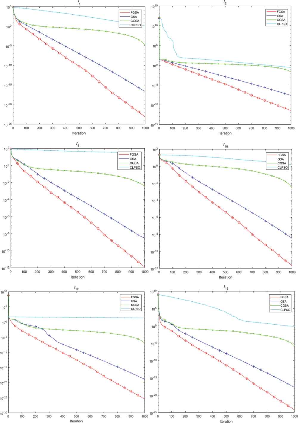
Comparison of performance of
For CGSA and CLPSO, the results of FGSA are better in most functions. In particular, the mean, median and variance of
The progress of GSA, CGSA and CLPSO for
The non-parametric statistical method Wilcoxon test was used to make a compete comparison. Table 4 lists the results of the Wilcoxon test on every test function between FGSA and the other algorithms. Rows “+,” “=” and “−” denote the number of test functions of the other algorithms that FGSA performs better than, almost the same as, and worse than, respectively. Row “Score” indicates the difference between the number of “1”s and “−1”s. It is used to make an overall comparison between two algorithms.
| Function | FGSA | GSA |
CGSA |
CLPSO |
|---|---|---|---|---|
| Wilcoxon | Wilcoxon | Wilcoxon | ||
| + | + | + | ||
| + | + | + | ||
| + | − | = | ||
| + | + | + | ||
| + | − | = | ||
| = | = | + | ||
| − | = | − | ||
| = | = | − | ||
| − | − | − | ||
| + | + | + | ||
| − | − | − | ||
| + | + | + | ||
| + | + | + | ||
| = | = | − | ||
| = | − | − | ||
| + | 8 | 6 | 7 | |
| = | 4 | 4 | 2 | |
| − | 3 | 5 | 6 | |
| Score | 5 | 1 | 1 |
GSA, gravitational search algorithm; FGSA, fuzzy GSA.
The Wilcoxon test of the best results for 15 benchmark function.
For example, FGSA outperforms GSA on 8 functions (
4.1. Comparison with the Latest GSA Variants
To further validate the performance of the proposed algorithm, the three latest GSA variants, i.e., NFGSA [21], PSGSA [21] and EKRGSA [20], are selected for comparison.
In all algorithms, the test functions are the same as in Table 2. The number of agents is 50 (N = 50). The dimension of the test function is set to 30, the maximum number of iterations is 1000 and
Table 5 illustrates that the mean of FGSA is the best for
| Function | FGSA | NFGSA | PSGSA | EKRGSA | |
|---|---|---|---|---|---|
| Mean | 6.74E−24 | 7.51E−23 | 1.04E−02 | 3.68E−19 | |
| Mean | 3.55E−12 | 7.69E−09 | 3.77E−02 | 3.74E−09 | |
| Mean | 1.05E+02 | 9.13E +01 | 2.72E+02 | 2.46E+03 | |
| Mean | 1.26E−12 | 3.42E−08 | 1.67E−02 | 2.16E−08 | |
| Mean | 2.66E+01 | 2.50E+01 | 5.53E+01 | 2.457E+01 | |
| Mean | 0 | 0= | 3.33E−02 | − | |
| Mean | 4.57E−02 | 5.06E−02 | 1.05E−01 | 6E−02 | |
| Mean | −2.928E+03 | −2.68E+03 | −3.39E+03 | − | |
| Mean | 2.69E+01 | 2.33E+01 | 2.13E+01 | − | |
| Mean | 2.08E−12 | 5.16E−12 | 1.48E−02 | 3.61E−10 | |
| Mean | 2.06E+01 | 1.50E+00 | 1.01E+01 | − | |
| Mean | 4.32E−26 | 2.07E−02 | 1.17E−02 | 1.91E−21 | |
| Mean | 6.53E−25 | 1.10E−03 | 1.30E−01 | 3.13E−20 | |
| Mean | 3.506 | 4.32 | 5.93 | 1.02 | |
| Mean | 2.11E−03 | 2.78E−03 | 4.52E−03 | 9.05E−04 |
The best results of 15 benchmark function with NFGSA, PSGSA and EKRGSA.
4.2. Discussion
To set the parameters of GSA more reasonably, a fuzzy system with twelve fuzzy rules is introduced. However, the setting of the three input parameters needs to confirm the rationality. Thus, an experiment is designed to test the performance of three different combinations of input parameters:
| Function | SD + t | ZM + t | SD + ZM + t |
|---|---|---|---|
| 2.91E−21 | 1.43E−23 | 6.74E−24 | |
| 6.99E−11 | 1.60E−11 | 3.55E−12 | |
| 1.83E+02 | 1.93E+02 | 1.05E+02 | |
| 2.73E−11 | 1.67E−12 | 1.26E−12 | |
| 2.68E+01 | 2.88E+01 | 2.66E+01 | |
| 0 | 0 | 0 | |
| 3.98E−02 | 1.96E−02 | 4.57E−02 | |
| −2.84E+03 | −2.73E+03 | −2.93E+03 | |
| 2.95E+01 | 1.91E+01 | 2.69E+01 | |
| 3.80E−11 | 2.77E−12 | 2.08E−12 | |
| 1.60E+01 | 1.15E+01 | 2.06E+01 | |
| 1.69E−23 | 8.48E−26 | 4.32E−26 | |
| 2.27E−22 | 1.34E−24 | 6.53E−25 | |
| 5.17E+00 | 3.91E+00 | 3.82E+00 | |
| 3.27E−03 | 3.27E−03 | 2.11E−03 |
Mean of three ways of input parameters.
The average of the 25 best fitness values is chosen as the standard for testing the pros and cons. The combination of
The inference mechanism behind these fuzzy rules in Table 1 is herein explained. The process of controlling parameters by the corresponding fuzzy rules for
| Inputs | 199 | 200 | 201 | 499 | 500 | 501 | 799 | 800 | 801 | |
| 0.470 | 0.580 | 0.294 | 0.394 | 0.228 | 0.433 | 0.458 | 0.430 | 0.452 | ||
| 0.746 | 0.903 | 0.276 | 0.656 | 0.367 | 0.603 | 0.405 | 0.177 | 0.377 | ||
| Outputs | 25 | 25 | 25 | 31 | 40 | 25 | 11 | 11 | 11 | |
| 29.49 | 29.47 | 28.36 | 28.76 | 28.31 | 29.28 | 29.50 | 29.49 | 29.50 | ||
| Corresponding rule | 1 | 1 | 3 | 6 | 7 | 5 | 12 | 12 | 12 | |
Control parameters by corresponding fuzzy rules for
Due to the addition of a fuzzy system, the computational cost may be slightly worse. Nowadays, the performance of computer increasingly becomes improved. The gap of response time between FGSA and GSA is within seconds. However, we admit that our proposed algorithm has increased some computational cost. This is the limitation of the paper.
5. CONCLUSIONS
The idea of intelligently controlling the parameters of GSA is introduced, and a fuzzy system is designed for this purpose. In this article, an improved idea of controlling the important parameters of GSA is proposed, which shows that a fuzzy inference system containing 12 fuzzy rules can be used to control the parameters
The new strategy gives GSA a higher convergence rate and the ability to escape the local minimum. A balance between exploration and exploitation is also realized. The performance of FGSA is examined on fifteen well-known standard functions. The experimental results are compared with those of the original GSA, CGSA, CLPSO, NFGSA, PSGSA and EKRGSA. The results indicate that FGSA achieves superior performances on most functions.
CONFLICT OF INTEREST
The authors declare no conflict of interest.
AUTHORS' CONTRIBUTIONS
Xianrui Yu conceived the research, drafted the manuscript and performed the experiments; Xiaobing Yu edited, and revised the manuscript. Chenliang Li and Hong Chen designed the experiments and analyzed the data.
ACKNOWLEDGMENTS
This research was funded by the National Natural Science Foundation of China (No.71974100, No.71503134), Natural Science Foundation of Jiangsu Province (No. BK20191402), Major Project of Philosophy and Social Science Research in Colleges and Universities of Jiangsu province (2019SJZDA039), Key Project of National Social and Scientific Fund Program (16ZDA047), Qing Lan project (R2019Q05), Postgraduate research and innovation plan project of Jiangsu Province (SJKY19_0983) and National Undergraduate Training Program for Innovation and Entrepreneurship (201910300016Z), the Joint Open Project of KLME & CIC-FEMD, NUIST (KLME202004).
REFERENCES
Cite this article
TY  - JOUR
AU  - Yu Xianrui
AU  - Yu Xiaobing
AU  - Li Chenliang
AU  - Chen Hong
PY  - 2020
DA  - 2020/06/25
TI  - An Improved Parameter Control Based on a Fuzzy System for Gravitational Search Algorithm
JO  - International Journal of Computational Intelligence Systems
SP  - 893
EP  - 903
VL  - 13
IS  - 1
SN  - 1875-6883
UR  - https://doi.org/10.2991/ijcis.d.200615.001
DO  - 10.2991/ijcis.d.200615.001
ID  - Xianrui2020
ER  -