
A New Hybrid Metaheuristic Algorithm for Multiobjective Optimization Problems
 , M.A. El-Shorbagy1, 2, , A.A. Mousa1, 3, , I.M. El-Desoky1
- DOI
- 10.2991/ijcis.d.200618.001How to use a DOI?
- Keywords
- Sine-cosine algorithm; Nondominated sorting genetic algorithm; Multiobjective optimization problems; The economic emission dispatch problem; TOPSIS
- Abstract
The elitist nondominated sorting genetic algorithm (NSGA-II) is hybridized with the sine-cosine algorithm (SCA) in this paper to solve multiobjective optimization problems. The proposed hybrid algorithm is named nondominated sorting sine-cosine genetic algorithm (NS-SCGA). The main idea of this algorithm is the following: NS-SCGA integrates the merits of exploitation capability of NSGA-II and exploration capability of SCA for a better search ability and speeds up the searching process. The performance of NS-SCGA is tested on the set of benchmark functions provided for CEC09. The NS-SCGA results are compared with other recently developed multiobjective algorithms in terms of convergence, spacing, and spread of the obtained nondominated solutions to the true Pareto front. The statistical analysis of the results obtained is performed by nonparametric Friedman and Wilcoxon signed-rank tests. The results prove that NS-SCGA is superior to or competitive with other multiobjective optimization algorithms considered in the comparison. Furthermore, the economic emission dispatch problem (EEDP) is solved by NS-SCGA. The operating cost (fuel cost) and pollutant emission of the standard IEEE 30-bus network with six generating units are minimized simultaneously by the NS-SCGA considering the losses. The results show the superiority of NS-SCGA and confirm its ability in solving EEDP. Finally, TOPSIS technique is applied to choose the best compromise solution from the obtained Pareto-optimal solutions of EEDP according to the decision-maker's preference.
- Copyright
- © 2020 The Authors. Published by Atlantis Press SARL.
- Open Access
- This is an open access article distributed under the CC BY-NC 4.0 license (http://creativecommons.org/licenses/by-nc/4.0/).
1. INTRODUCTION
In the real world, many engineering, science, finance, economics, and logistics optimization problems usually have more than one conflict objective. Problems of this kind are named as multiobjective optimization problems (MOPs).
MOPs are different from single-objective optimization, as there is no single solution that optimizes all objective functions simultaneously. It makes solving MOPs a challenging job, because of the conflicting nature of objective functions (improving one objective leads commonly to the deterioration of another, a.k.a improving one worsens others). In addition, the obtained set of solutions from solving MOPs (Pareto-optimal) has main features such as the following: each solution produces trade-offs between the different objectives, and no solution is subaltern to the other solutions [1].
Different conventional algorithms have been developed to solve MOPs such as the following: the goal programming, the hierarchical optimization algorithms, the ε-constraint technique, and the objective weighted method [2]. These techniques converted the vector of objectives of MOP into a single objective by generating one particular nondominated solution at a time. The conventional algorithms suffer from some drawbacks, such as the differentiation requirements of the objective function and constraints, the need for a good initial point, the expensive computation for Jacobian and/or Hessian [1,3]. Also, these methods are usually inefficient in case of some objectives involving concavity, discontinuity, uncertainty, and noise in their search space [4]. Therefore, they cannot be used universally in optimizing the complex MOPs.
Therefore, over the past two decades, much emphasis has been laid on developing metaheuristic methods to yield a computationally efficient and convergent procedure. Among these metaheuristic methods are evolutionary algorithms (EAs) and intelligent swarm algorithms [5]. Most of the metaheuristic algorithms can obtain the Pareto-optimal solutions of MOPs, which are difficult to obtain by the conventional algorithms within a reasonable computation time, as proven in [5].
The most popular metaheuristic algorithms for solving MOPs are the following: multiobjective genetic algorithm (MOGA) [6,7], nondominated sorting genetic algorithm (NSGA-II) [8], Niche Pareto genetic algorithm (NPGA) [9], a multiobjective differential-evolution algorithm (MO-DEA) [10], strength Pareto evolutionary algorithm (SPEA) [11], SPEA2 [12], Pareto archived evolutionary strategy (PAES) [13], multiobjective evolutionary algorithm (MOEA) based on decomposition (MOEA/D) [14], Liu Li algorithm [15], indicator-based EA (IBEA) [16], archived multiobjective simulated annealing (AMOSA) [17], multiobjective particle swarm optimization (MOPSO) algorithm [18], clustering multiobjective EA (clustering MOEA) [19], multiple trajectory search (MTS) [20], a multiobjective teaching learning based optimization (MO-TLBO) algorithm [21], multiobjective firefly algorithm for continuous optimization [22], multiobjective cuckoo search [23], a multiobjective ant colony algorithm [24], multiobjective optimization (MO) algorithm based on artificial algae (MO-AAA) [1], multiobjective ant lion optimizer [25], water cycle algorithm [26], multiobjective grey wolf optimizer (MOGWO) [27], dragonfly algorithm [28], multiobjective sine-cosine algorithm (SCA) [29,30], and others; it is difficult to mention all.
In addition, the hybrid algorithms have also been developed and applied to a variety of MOPs and their application such as [31–36]. Hybrid algorithms can be more efficient than the basic versions of the basic approaches, because of the fact that the hybrid algorithm benefits from all the advantages of the basic algorithms. Many researchers proposed hybrid metaheuristic algorithms for this aim. The literature proves that hybridizing metaheuristic techniques is one of the ways of using the advantages of many techniques. It also aids in developing an efficient technique to solve optimization problems, such as sine-cosine crow algorithm [37], NSGA-II/EDA hybrid EA [38], nondominated sorting moth-flame optimization (NS-MFO) [39], K-means-clustering-based EA [40], and GA-based clustering technique [41].
Genetic algorithms (GAs) are the most popular metaheuristic algorithms that introduced at 1975. GAs are well suited to solve MOPs by searching the Pareto front step by step. The primary reason for using GA for MO is its ability to deal with a set of potential solutions (population) and finding Pareto-optimal solutions at each simulation run. The ability of GA in the convergence and searching for the global optimum makes it possible to obtain a diverse solutions' set for the complex problems in multimodal, nonconvex, and discontinuous solution spaces [42]. Therefore, for MOPs, a variety of GA methods can be suggested: random weighted GA (RWGA), NPGA, nondominated sorting GA (NSGA), MOGA, SPEA, and NSGA-II. Of all the aforementioned methods, NSGA-II is a recently and efficiently well-known MOEA which has captured more attention due to its efficiency in producing better Pareto front for any number of objectives [43].
NSGA-II, introduced in 2000 [8], is an improved version of NSGA. NSGA-II uses the elitist technique, which consists of sorting the population at different “fronts” using the nondominated ranking technique with a particular bookkeeping strategy. The crowding distance (CRD) sorting is a secondary ranking that measures the population density around each solution and sorts the individuals, which enter the same front. The best solutions are then chosen according to nondominance and diversity. NSGA-II is computationally fast, incorporates elitism, and converges better in the obtained Pareto front compared to other MOEAs. The NSGA-II has been proved as a very efficient multiobjective GA which had been used successfully in solving various MOPs [44–47]. The algorithm's calculation performance depends on the optimizing strategy inside of the algorithm itself. Besides this, the calculation performance of one algorithm varies when dealing with various optimization problems. So, various researchers presented some improvement strategies into the NSGA-II to deal with the shortcomings when solving some complex optimization problems.
SCA is a recent metaheuristic algorithm presented by Mirjalili in 2016 [48]. SCA proved its efficiency in solving single-objective optimization [48]. SCA updates its solutions according to the trigonometric sine and cosine functions, where it oscillates around the best solution. This algorithm has been studied and investigated by many researchers and applied to solve many problems in different fields [29,49–52] due to its higher exploration capability, simple implementation, and less parameter setting. But SCA suffers from slow convergence and speed, low optimization precision, and weak exploitation capability. The algorithm is often trapped in local minima [53]. According to this, in the last two years, many researches proposed various improvements in SCA from different perspectives to handle these drawbacks [54–56].
In this article, a novel optimization algorithm called nondominated sorting sine-cosine genetic algorithm (NS-SCGA) is presented for solving MOPs. The proposed algorithm combined NSGA-II and SCA to integrate the merits of both techniques. The main idea of the proposed algorithm is the following: NS-SCGA integrates the merits of exploitation capability of NSGA-II and exploration capability of SCA for a better search ability as well as speeding up the searching process. The nondominated sorting and CRD techniques of NSGA-II divide the population into several ranks, which ensure Pareto dominance and solution diversity in NS-SCGA. The population evolves using the SCA mechanism along with the genetic operators, which integrate the merits of exploitation capability of genetic operators and the exploration capability of SCA. The search accuracy and performance of the NS-SCGA are verified on the set of benchmark functions provided for the 2009 IEEE Congress on Evolutionary Computation (CEC09). They are also compared with other recently developed multiobjective algorithms in terms of convergence, spacing, and spread of obtained nondominated solutions along the true Pareto front. The Lexicographic ordering (LO) is used to assess the overall performance of the proposed NS-SCGA among the compared techniques. The statistical analysis of the experimental results is also carried out by nonparametric Friedman and Wilcoxon signed-rank tests. The computational results prove that the NS-SCGA is superior to or competitive with other MO algorithms considered in the comparison.
The economic emission dispatch problem (EEDP) is a crucial task in the planning and operation of the power systems [57]. EEDP in power systems is a task of the determination of an optimum schedule of a generation of the generating units to minimize the total generation cost and pollutants emission within the constraints of the power system. EEDP is becoming more and more worthwhile for not only resulting in great economic benefit but minimizing the emission of pollutants also. EEDP is considered a highly constrained conflicting MOP, and it is very complex to solve due to its nonlinearity nature.
Different algorithms have been presented in the literature to solve EEDP including conventional optimization methods and metaheuristic algorithms. Among the conventional optimization algorithms which had been used in solving EEDP are the following: a linear programming method [58], weighted sum method [59], lambda iteration method [60], ε-constraint method, Lagrangian multiplier method [61], and quadratic programming [62]. But these conventional techniques need the curves of incremental cost to be piece-wise or increasing monotonically linear. But, virtually, the input characteristics of the generators are highly nonsmooth and nonlinear [63]. In addition, due to the nonlinearity and nonconvexity that arise from the effect of the valve point, using these conventional techniques is not recommended and is not suitable for a complex EEDP [64].
On the other hand, some metaheuristic algorithms, especially EAs and swarm intelligence algorithms, were used to solve EEDP [64–67]. Here, the NS-SCGA which is a hybrid algorithm of two metaheuristic search techniques, is implemented to solve the standard IEEE 30-bus with the six-generator network. The proposed NS-SCGA is compared to other MO algorithms, and the effectiveness of NS-SCGA in solving the EEDP is demonstrated.
Finally, Technique for Order Performance by Similarity to Ideal Solution (TOPSIS) is used to help the decision-maker (DM) to identify the best compromise solution from the nondominated solutions obtained by the proposed NS-SCGA [68]. TOPSIS takes into account the relative priorities of the two objective functions (minimum fuel cost and the minimum emission) in the Pareto-optimal solutions on the basis of the DM perceptions. TOPSIS technique is based upon distance maximization from a nadir point (NP) and distance minimization from the negative ideal solution simultaneously. A NP is constructed by the worst objective values of the solutions of the entire Pareto-optimal set.
The main contributions of the present article are as follows:
A novel optimization algorithm, called NS-SCGA, is presented and evaluated.
A comparative study of the optimization results using NS-SCGA is presented to 20 benchmark multiobjective problems.
The results of 20 benchmark functions obtained by NS-SCGA are compared with other newly developed algorithms, and the LO, Friedman test and Wilcoxon signed-rank test are used for evaluating the overall performance of the comparing algorithms.
NS-SCGA is applied to EEDP and the results are compared with other optimization algorithms.
The best compromise solution of EEDP has been extracted by the TOPSIS technique from nondominated solutions according to the DM's preference.
The rest of this paper is organized as follows: The preliminaries about the MO are briefly studied in Section 2. Section 3 describes the NSGA-II briefly. Section 4 includes the description of the SCA. The explanation about NS-SCGA is given in Section 5. Section 6 presents and discusses the results. Finally, Section 7 includes the conclusion of this paper.
2. MULTIOBJECTIVE OPTIMIZATION PROBLEMS
The MO deals with more than one objective function. In order to solve the MOPs, all objectives functions must be optimized simultaneously. In general, there are two categories of MOPs: one is unconstrained MOPs (UCMOPs) and the other is constrained MOPs (CMOPs). The general formulation of the MOP is given by [69]
In MO, the objectives are often conflicting and need special considerations. Therefore, comparing the MOPs solutions by the relational operators is no longer effective, because of the presence of more than one criterion for a comparison [70]. Consequently, other operators are needed to find out and measure how much a solution is better than another. The Pareto dominance is the most widely used operator for comparing the MOPs solutions which can be defined as follows [71]:
Pareto Dominance. It is the case if q and p are two feasible solutions belonging to
The Pareto-optimal solution can be defined as follows:
Pareto-Optimal Solution. The feasible solution,
The set of all Pareto-optimal solutions is called the Pareto-optimal set (POS), while the Pareto-optimal front (POF):
3. THE ELITIST NSGA-II
NSGA-II is a population-based algorithm, which is widely used in solving MOPs [8]. In this algorithm, the individuals are divided into nondominated layers on the basis of the concept of Pareto and sorting nondominated solutions as graphically explained in Figure 1.
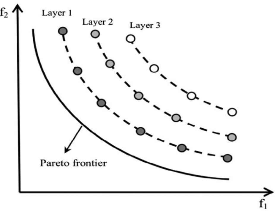
The schematic view of grouping the solutions in different layers in nondominated sorting genetic algorithm (NSGA-II) [73].
In NSGA-II, the offspring population
3.1. Sorting the Individuals into Nondominated Layers (The Fast Nondominated Sorting Technique)
For each solution j in the intermediate population (
Step 1. Evaluate all the objective functions for each solution.
Step 2. Assign a domination count zero for all the solutions and put them in the first nondominated layer.
Step 3. For each individual j with
Step 4. The above step is repeated for each solution of 2nd nondomination layer to find the 3rd layer; thereafter, the procedure is repeated until all the population are assigned into different nondomination layers.
The elitist nondominated sorting technique.
For each individual j in the 2nd or higher level of nondomination layer, the domination count
Therefore, if two individuals (i and j) with different layers are compared, the individual with a better or lower layer is prioritized. But if both individuals belong to the same layer (
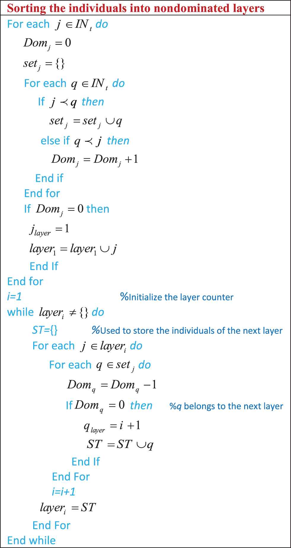
3.2. The CRD
The CRD is assigned to each individual i in the population with the goal of measuring the density of individuals surrounding it. Therefore, the
Step 1. Determine the number of individuals in each layer as
Step 2. Assign
Step 3. Sort the individuals in the layer in the worst order of
Step 4. Assign infinity CRD to the first and the last individuals in the sorted list, for each objective function (
Step 5. Assign CRD for the other individuals in the sorted list i = 2 to (h-1) for each objective by
The pseudocode of crowding distance computation.
The crowding-comparison operator (
The crowding-comparison operator chooses the solutions from the least crowded region, which guarantees the diversity in the population.
4. SINE-COSINE ALGORITHM
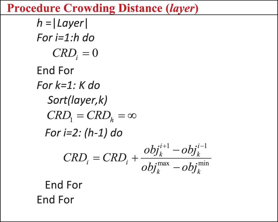
SCA is a population-based algorithm which is based on sine and cosine mathematical functions for solving optimization problems. SCA initiates the search process with a random agent set, which is updated in each generation by using the mathematical expressions based on sine and cosine functions. The position of each individual is updated by the following equations [48]:
As shown in (5), the deterministic parameter
- where c is constant, q is the current iteration, and
Finally,
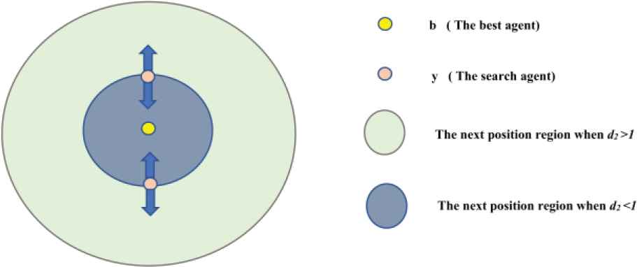
Effect of sine and cosine components in (5).
The general steps of SCA are implemented as follows:
Initialize random solutions set (search agents) inside the range of upper and lower limits of decision variables.
While (q < qmax)
Do
Evaluate the objective functions of each solution.
Identify the best individual according to the objective function (
Update the deterministic parameter
Update the individual position through. (5).
End
Save the best individual obtained so far as the optimal solution
5. THE NS-SCGA
This section introduces the NS-SCGA. NS-SCGA aims to integrate the merits of exploration capability of SCA and exploitation capability of NSGA-II to quicken the process of searching, avoid getting stuck in local minima, and speed up the convergence to best solutions in a reasonable time. In NS-SCGA, the nondominated sorting and CRD techniques of NSGA-II divide the population into several ranks, which ensure solution diversity and Pareto dominance in NS-SCGA. Meanwhile, the population is evolved by the SCA mechanism along with the genetic operators, which integrates the merits of exploitation capability of genetic operators and the exploration capability of SCA. In NS-SCGA, the initial set of candidate solutions is generated and iteratively updated. Each new generation is produced by stochastically removing less desired solutions and introducing small random changes. The population of the solutions is subjected to selection based on CRD operator and crossover and mutation operators and updating formula of SCA. As a result, the population will gradually evolve toward an optimal solution. Therefore, the combination of the two well-known search strategies in the optimization field by this different technique aims to speed the process of searching, speed up the convergence to best solutions in a reasonable time, and avoid getting stuck in local minima, which can make a contribution in the field of multi-objective optimization. The basic steps of NS-SCGA are shown in Figure 5 and can be illustrated as follows:
- Step 1
(Initialization):
Firstly, initialize the set of parameters which are the following:
Npop: the size of population
Crossover-probability pc
Mutation-probability pm
Secondly, initialize the parent population (
- Step 2
(Evaluation):
Once the population is initialized, the objective functions of each individual are evaluated.
- Step 3
(Generating Offspring Population):
Divide
- Step 4
(Evaluation):
Once the offspring population is generated, the objective functions of each individual are evaluated.
- Step 5
(Merge):
Merge
- Step 6
(Sorting the Population-Based on Crowding-Comparison Operator):
Compute Layer and CRD for each individual of
- Step 7
(Generate the New Population):
Choose the new population (Npop) solutions from the sorted
- Step 8
(Termination Condition):
When the termination condition (maximum number of function evaluations [NFEs] or maximum number of generations) has been satisfied, the algorithm is stopped.
If the termination condition is not satisfied, the selected Npop solutions are assigned as
- Step 9
(The Optimal Pareto Front)
When the termination condition is satisfied the nondominated solutions in the first layer are selected and assigned as the optimal Pareto solution.
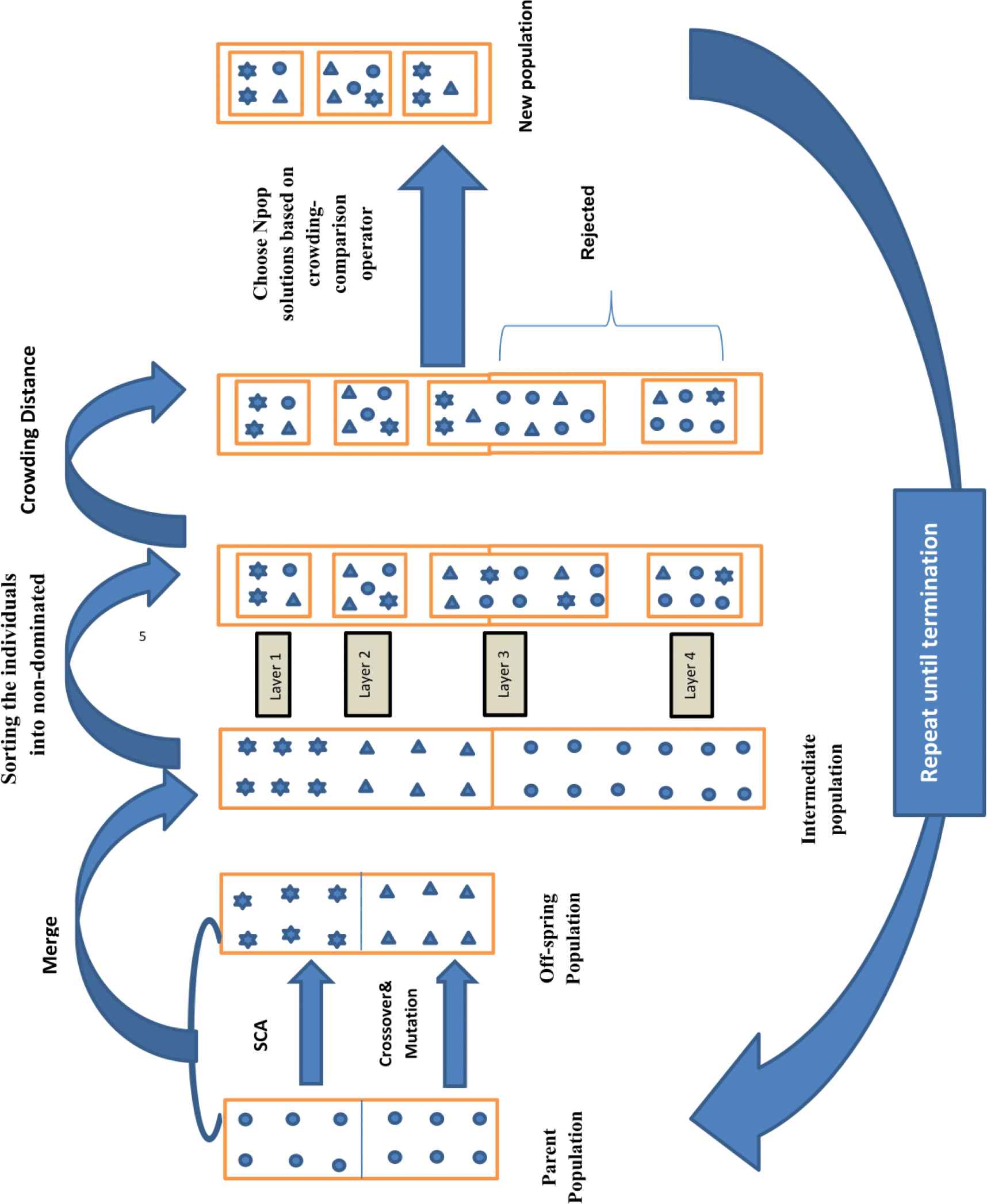
The framework of nondominated sorting sine-cosine genetic algorithm (NS-SCGA).
6. EXPERIMENTAL RESULTS
The performance of NS-SCGA is benchmarked by three main groups of test function which are as follows:
Unconstrained multiobjective test functions: 10 unconstrained benchmark functions from the CEC09 test suite (UF1-UF10).
Constrained multiobjective test functions: 10 constrained benchmark functions from the CEC09 test suite (CF1-CF10).
Engineering application: The EEDP.
The NS-SCGA is coded in MATLAB 2018. The parameters of NS-SCGA used are given in Table 1. The NS-SCGA is implemented 30 times for each problem and the average results of the NS-SCGA are compared with the results of the other techniques available in the literature in terms of three commonly used performance metrics: inverted generational distance (IGD), maximum spread (MS), and spacing metric (SP).
| Pc | 0.95 |
|---|---|
| Crossover operator | Single_point |
| Pm | 0.09 |
| Mutation operator | Real_value |
| NS-SCGA iterations | 100–500 |
NS-SCGA, nondominated sorting sine-cosine genetic algorithm.
The description of the parameters set.
6.1. Performance Metrics
In order to validate the quality of the Pareto-optimal solutions obtained by the NS-SCGA, both quantitative and qualitative metrics are employed, including IGD, MS, and SP. For quantifying the convergence, IGD is employed [1,77], where SP [78] and MS [79] have been employed to quantify the distribution of the obtained Pareto-optimal front (coverage).
Inverted Generational Distance (IGD): IGD is used to quantify the convergence by calculating the distance of the obtained Pareto front (OPF) by the proposed algorithm from the true Pareto front (TPF). A small value of IGD denotes that the OPF closely approaches the TPF. The mathematical equations of this performance metric are given by
where TPF is the set of uniformly distributed points along true Pareto front and OPF is the set of the obtained Pareto-optimal solutions by the proposed algorithm. FurthermoreSP: SP is used to measure the extent of the spread of the nondominated solutions throughout the Pareto front (i.e., it describes the distribution of nondominated solutions vectors). Through comparison with the true Pareto, coverage degree or distribution of nondominated solution vectors searched by algorithm could be
where
The lower value of SP indicates a better uniform distribution in OPF. As the smaller value of SP indicates the better distribution of the current solution set of the algorithm as the zero value of SP indicates that all the Pareto points on the front are equidistant to each other and the Pareto points are evenly distributed on the front
MS: MS is used to measure the maximum extension covered by the nondominated solution in the Pareto front. The mathematical equation of this performance metric is
where
A higher value of MS indicates that the nondominated solutions covered a large area of Pareto front.
6.2. Results of Unconstrained (CEC09) Benchmark Functions
To investigate the NS-SCGA performance, unconstrained test suites CEC09 have been employed. Among all the ten unconstrained benchmark problems, UF1 to UF7 are biobjective and UF8 to UF10 are triobjective optimization problems. The mathematical equations of these test functions are given in [80].
The maximum NFEs is set as 300000. The proposed NS-SCGA is compared with another 11 newly developed algorithms for MOPs in terms of the average value of IGD obtained in 30 independent runs. These algorithms are MO-TLBO [21], MOEA/D [14], MTS [20], MOEA/D with guided mutation and priority update (MOEADGM) [81], dynamical MOEA with decomposition technique (DMOEADD) [82], multiobjective artificial bee colony algorithm (MOABC) [83], Liu Li algorithm [15], hybrid NSGA-II with adaptive operators selection (HNSGA) [84], a new decomposition-based MOEA with the ε-constraint framework (DMOEA-εC) [85], adaptive cross-generation differential evolution (ACGDE-NSGA-II) [86], and MO-AAA [1]. The computational results of UF1 to UF10 benchmark functions are given in Table 2. Moreover, NS-SCGA is compared with another three recent algorithms, which solved unconstrained CEC09 in terms of the average value of SP and MS obtained in 30 independent runs in Table 3. These algorithms include enhanced multiobjective particle swarm optimization (MOPSO+EPD) [87], MOGWO [27], and multiobjective grasshopper optimization algorithm (MOGOA) [88]. The best Pareto-optimal fronts obtained by the NS-SCGA are given in Figure 6.
| MO-AAA | MO-TLBO | MOEA/D | MTS | DMOEADD | MOABC | Liu Li Algorithm | MOEADGM | HNSGA | DMOEA-εC | ACGDE-NSGA-II | NS-SCGA | |
|---|---|---|---|---|---|---|---|---|---|---|---|---|
| UF1 | 0.003910 | 0.008790 | 0.004350 | 0.006460 | 0.01040 | 0.006180 | 0.007850 | 0.006200 | 0.01203 | 0.004407 | 0.05280 | 0.003840 |
| UF2 | 0.006720 | 0.007840 | 0.006790 | 0.006150 | 0.006790 | 0.004840 | 0.01230 | 0.006400 | 0.003897 | 0.006530 | 0.02050 | 0.003700 |
| UF3 | 0.07620 | 0.06930 | 0.007420 | 0.05310 | 0.03340 | 0.05120 | 0.01500 | 0.04290 | 0.02875 | 0.007209 | 0.09470 | 0.01290 |
| UF4 | 0.03560 | 0.07010 | 0.06390 | 0.02630 | 0.04270 | 0.05800 | 0.04350 | 0.04760 | 0.04121 | 0.06017 | 0.04100 | 0.02540 |
| UF5 | 0.04130 | 0.09790 | 0.1810 | 0.04490 | 0.3150 | 0.07780 | 0.1620 | 1.790 | 0.3792 | 0.3845 | 0.2870 | 0.04122 |
| UF6 | 0.04820 | 0.05530 | 0.005870 | 0.05920 | 0.06670 | 0.06540 | 0.1760 | 0.5560 | 0.1508 | 0.2662 | 0.1576 | 0.004801 |
| UF7 | 0.006420 | 0.06800 | 0.004440 | 0.04080 | 0.01030 | 0.05570 | 0.007300 | 0.007600 | 0.009700 | 0.004079 | 0.02620 | 0.004022 |
| UF8 | 0.05980 | 0.09930 | 0.05840 | 0.1130 | 0.06840 | 0.06730 | 0.08240 | 0.2450 | 0.08169 | 0.05284 | 0.1383 | 0.09634 |
| UF9 | 0.2000 | 0.1640 | 0.07900 | 0.1140 | 0.04900 | 0.06150 | 0.09390 | 0.1880 | 0.1120 | 0.04290 | 0.1776 | 0.03990 |
| UF10 | 0.5120 | 0.1790 | 0.4740 | 0.1530 | 0.3220 | 0.1950 | 0.4470 | 0.5650 | 0.3165 | 0.02240 | 0.6440 | 0.2873 |
IGD values for different CEC09 unconstrained test functions obtained by nondominated sorting sine-cosine genetic algorithm (NS-SCGA) and other techniques in 30 independent runs.
| MOGOA |
MOGWO |
MOPSO+EPD |
NS-SCGA |
|||||
|---|---|---|---|---|---|---|---|---|
| MS | SP | MS | SP | MS | SP | MS | SP | |
| UF1 | 0.7270 | 0.001200 | 0.9268 | 0.01237 | 1.263 | 0.008000 | 1.401 | 0.001000 |
| UF2 | 0.8845 | 0.0007000 | 0.9097 | 0.01108 | 0.8640 | 0.008000 | 1.403 | 0.0009531 |
| UF3 | 0.6051 | 0.001900 | 0.9498 | 0.04590 | 1.406 | 0.007000 | 1.412 | 0.0005095 |
| UF4 | 0.9050 | 0.0001000 | 0.9424 | 0.009690 | 1.025 | 0.007000 | 1.232 | 0.0007899 |
| UF5 | 0.2379 | 0.0007000 | 0.3950 | 0.1523 | 1.275 | 0.005000 | 1.525 | 0.001300 |
| UF6 | 0.2525 | 0.0003000 | 0.6736 | 0.01446 | 0.6060 | 0.007000 | 1.031 | 0.007500 |
| UF7 | 0.8460 | 0.0001000 | 0.8013 | 0.008240 | 0.7860 | 0.007000 | 1.361 | 0.00009000 |
| UF8 | 0.4417 | 0.01750 | 0.4457 | 0.006870 | 4.065 | 0.02600 | 1.731 | 0.01250 |
| UF9 | 0.1938 | 0.01390 | 0.8399 | 0.01730 | 3.838 | 0.02300 | 1.724 | 0.01290 |
| UF10 | 0.3233 | 0.006700 | 0.2972 | 0.02523 | 2.913 | 0.01900 | 1.725 | 0.02990 |
SP and MS values for different CEC09 unconstrained test functions obtained by nondominated sorting sine-cosine genetic algorithm (NS-SCGA) and other techniques in 30 independent runs.
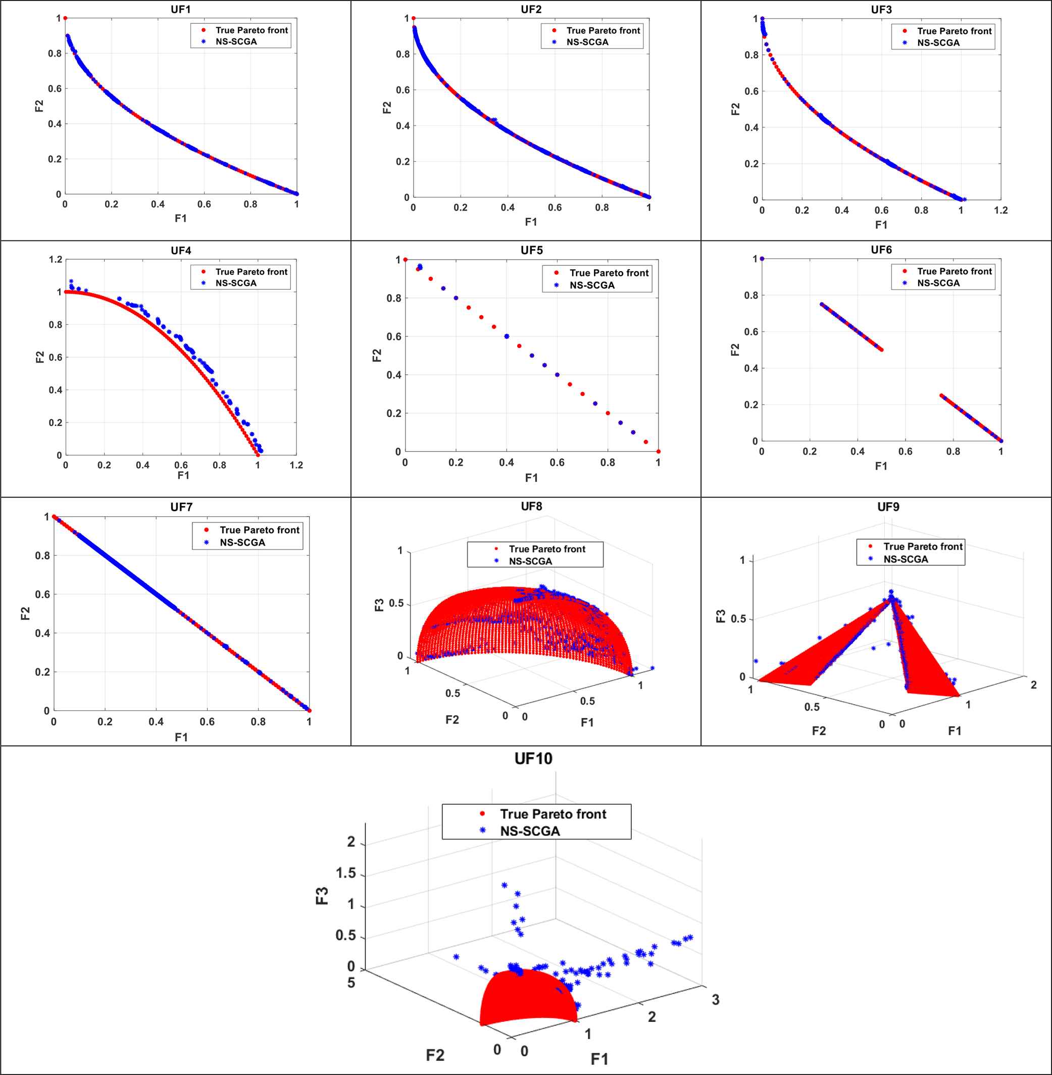
The obtained Pareto fronts by the nondominated sorting sine-cosine genetic algorithm (NS-SCGA) for CEC09 unconstrained benchmark functions.
It can be noticed that three other methods are used in the comparison between SP and MS values in Table 3, as IGD calculation has two formulas in the literature (the one which was used in formula 7 and the other one can be found in [27,87]).
The 11 techniques used in the comparison in Table 2 use the same formula which is used in calculating the IGD metric in this paper, while those 11 techniques did not calculate SP and MS metric. That is why we used the only three methods that were found in the literature which calculate SP and MS metrics for these benchmark functions in the comparison of the results of SP and MS metric. (Meanwhile, they did not use the same formula of IGD metric which is used in our work.)
Based on Table 2, the NS-SCGA showed improved average results in comparison to all other techniques across all test suites except for problems UF3, UF8, and UF10.
As shown in Table 2 in UF2, UF5, UF6, UF7, and UF9 function, the average value of IGD produced by NS-SCGA is better than the other techniques. Therefore, our algorithm outperforms the other techniques in these functions. As shown in Figure 6, the obtained Pareto fronts of these functions by the NS-SCGA show a good convergence and suitable distribution over the Pareto front.
Meanwhile, the NS-SCGA obtains a competitive result for UF1 and UF4 functions. Only MO-AAA obtains results comparable to the NS-SCGA, but the latter still produces slightly better solutions. The obtained Pareto front for UF1 and UF4 test functions represents good distribution and appropriate proximity in the objective space. But, for the UF3 function, the NS-SCGA is placed at the third rank in solving it. Only DMOEA-εc and MOEA/D algorithms give a good result compared to NS-SCGA. As shown in Figure 6, the obtained nondominated solutions of UF3 are uniformly distributed along the Pareto front. The UF8 is the first triobjectives benchmark function solved in this work. The NS-SCGA is ranked the eighth in solving UF8 among the competing algorithms. The MO-AAA, MOEA/D, DMOEADD, MOABC, Liu Li, HNSGA, and DMOEA-Εc algorithms obtained the best result for this benchmark function. However, the obtained Pareto front of UF8 shows that NS-SCGA obtained a set of solutions distributed appropriately in the three-dimensional objective space. Also, in the case of the UF10 benchmark function, MO-TLBO, MTS, MOABC, and DMOEA-c produced competitive performance. The proposed NS-SCGA obtained the fifth rank in solving this problem. Figure 6 shows that most of the portions of the Pareto front of UF10 are not covered successfully by NS-SCGA. Thus, the IGD value is a large value in the UF10 test problem.
This shows that, overall, the NS-SCGA has good convergence for unconstrained MOPs and rivals other techniques that we compared it against in these experiments. On the other hand, Figure 6 proves that the obtained Pareto-optimal solutions by the NS-SCGA tend to be closer to the true Pareto-optimal front. That is, the proposed NS-SCGA is capable of approximating the true Pareto front.
Note that MS with high values and SP with low values indicate that the obtained Pareto-optimal fronts have a more uniform distribution. It can be observed from Table 3 that our algorithm is superior in almost half of the benchmark problems. These results prove that the coverage of the obtained solutions by the NS-SCGA is of high distribution across all objectives of the benchmark functions. This can be observed as well in Figure 6 where the obtained solutions by the NS-SCGA are well-distributed on the majority of the benchmark functions.
As per the results of Tables 2 and 3 and Figure 6, it is proved that NS-SCGA is able to outperform other techniques in the majority of unconstrained benchmark problems and the obtained Pareto-optimal fronts are well spread across all objectives.
6.3. Results of Constrained (CEC09) Benchmark Functions
The performance of NS-SCGA in solving the CMOPs is evaluated by investigating constrained CEC09 test instances. Among the constrained CEC09 benchmark problems, CF1–CF7 are biobjective where CF8, CF9, and CF10 are triobjective problems. The mathematical equations of these test instances are available in [80]. The NFEs is set as 300000. The NS-SCGA is compared with eight other MO algorithms for CMOPs in terms of the average IGD value estimated in 30 independent runs. These algorithms include MTS [20], MOEADGM [81], Liu Li algorithm [15], differential evolution with self-adaptation and local search for constraint multiobjective optimization algorithm (DECMOSA-SQP) [89], NSGA-II with local search (NSGAIILS) [47], generalized differential evolution (GDE3), and MO-AAA [1]. The computational results of CF1 to CF10 benchmark functions are shown in Table 4. All the results except for the NS-SCGA were taken from [1] for the comparison purpose. The best obtained Pareto-optimal fronts by the NS-SCGA are given in Figure 7.
| MO-AAA | Liu Li Algorithm | DECMOSA-SQP | MTS | NSGAIILS | GDE3 | MO-TLBO | MOEADGM | NS-SCGA | |
|---|---|---|---|---|---|---|---|---|---|
| Cf1 | 0.06820 | 0.0008500 | 0.1080 | 0.01920 | 0.006920 | 0.02940 | 0.02490 | 0.01080 | 0.006000 |
| Cf2 | 0.003920 | 0.004200 | 0.09460 | 0.02680 | 0.01180 | 0.01600 | 0.01200 | 0.008000 | 0.003851 |
| CF3 | 0.04250 | 0.1830 | 1.000 | 0.1040 | 0.2400 | 0.1280 | 0.09800 | 0.5130 | 0.04170 |
| CF4 | 0.002810 | 0.01420 | 0.1530 | 0.01110 | 0.01580 | 0.007990 | 0.008680 | 0.07070 | 0.007100 |
| CF5 | 0.06230 | 0.1100 | 0.4130 | 0.02080 | 0.1840 | 0.06800 | 0.07640 | 0.5450 | 0.01579 |
| CF6 | 0.04010 | 0.01390 | 0.1480 | 0.01600 | 0.02010 | 0.06200 | 0.0640 | 0.2070 | 0.03003 |
| CF7 | 0.02880 | 0.1040 | 0.2600 | 0.02470 | 0.2330 | 0.04170 | 0.03330 | 0.5360 | 0.01120 |
| CF8 | 0.03110 | 0.06070 | 0.1760 | 1.090 | 0.1110 | 0.1390 | 0.2980 | 0.4060 | 0.02290 |
| CF9 | 0.07620 | 0.05050 | 0.1270 | 0.08510 | 0.1060 | 0.1150 | 0.08100 | 0.1520 | 0.05041 |
| CF10 | 0.09990 | 0.1970 | 0.5070 | 0.1380 | 0.3590 | 0.4920 | 0.3010 | 0.3140 | 0.1034 |
IGD values for different CEC09 constrained multiobjective optimization problems (CMOPs) obtained by nondominated sorting sine-cosine genetic algorithm (NS-SCGA) and other techniques in 30 independent runs.
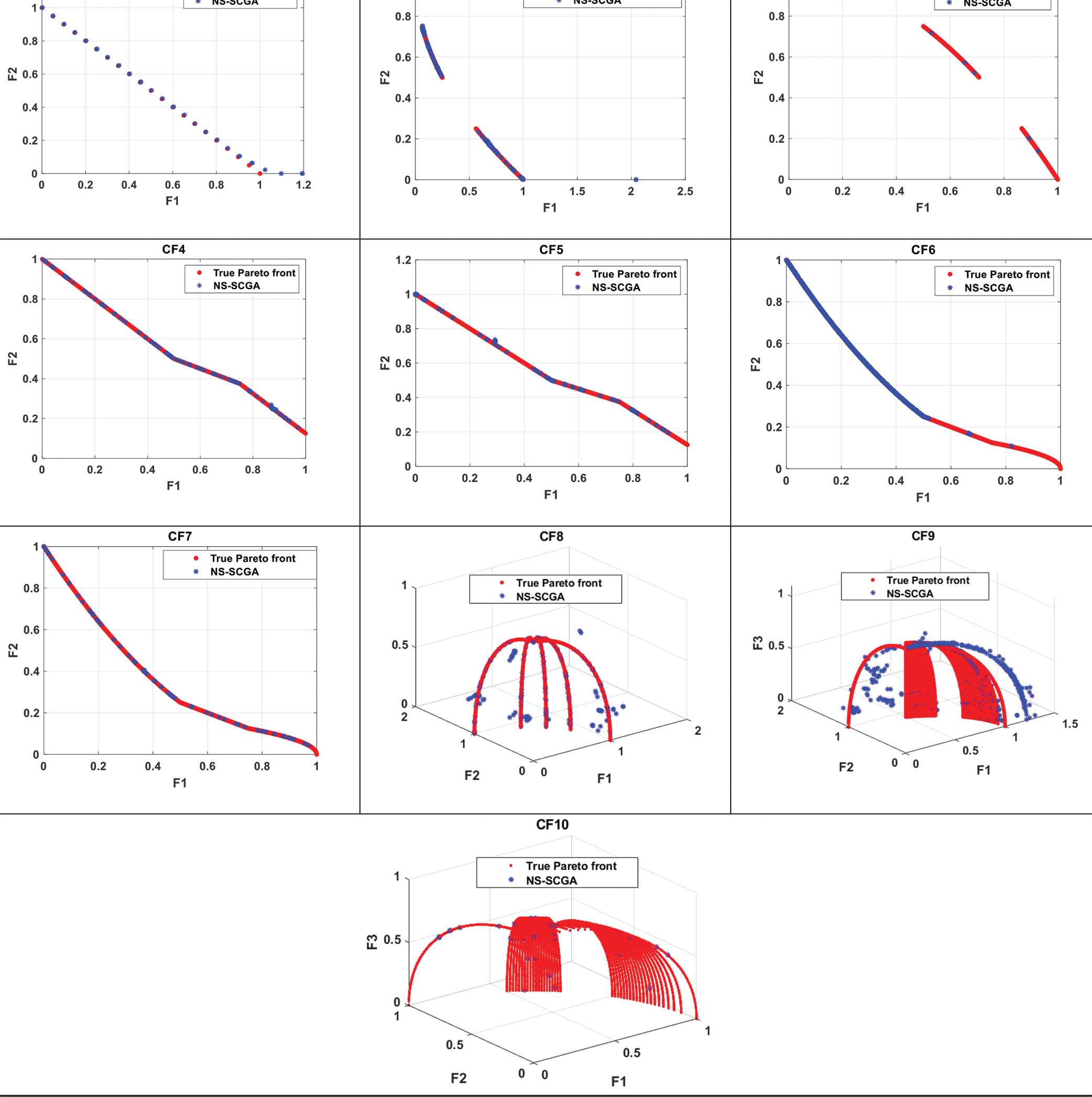
The Pareto front obtained by the nondominated sorting sine-cosine genetic algorithm (NS-SCGA) for CEC09 constrained multiobjective optimization problems (CMOPs).
As shown in Table 4, NS-SCGA obtains the best IGD values for all the constrained test functions, except in CF1, CF4, CF6, and CF10, for which MO-AAA and Liu Li algorithm obtain the best results for CF4&CF10 and CF1&CF6, respectively. However, the other compared algorithms do not perform as well as NS-SCGA, MO-AAA, and Liu Li algorithm. It is worth stressing that NS-SCGA outperforms MO-TLBO, MTS, NSGAIIlS, and MOEADGM, which are mainly designed for MOPs; therefore, their performance is not evaluated on CF test functions.
The approximated fronts obtained by NS-SCGA for each CF test functions are shown in Figure 7 with the true fronts. The obtained Pareto fronts by the NS-SCGA algorithm in the CF1, CF4, CF6, and CF10 test functions are well-converged and well-distributed also. Figure 7 proves that NS-SCGA is capable of converging to a certain degree to the true Pareto front. The proposed NS-SCGA performs well in CF8 and CF9 which are triobjective test functions. The Pareto-optimal solutions obtained by NS-SCGA cover almost the whole true Pareto fronts for the triobjective benchmark functions. The above results indicate that NS-SCGA is effective in solving CMOPs.
6.4. The LO for Unconstraint and Constrained Benchmark Problem
The LO [75] is used to assess the overall performance of the NS-SCGA between the 9 compared techniques in solving the constrained test problems and the 12 compared techniques in solving the unconstrained test functions. LO defines the overall rank of the compared techniques. For any test instance, the algorithm which occupies the 1st rank is the one which obtains the best value of average IGD for that function as compared to the rest of the techniques, and the next better performing algorithm obtains the 2nd rank, and so on. In this section, the ranks are assigned to the compared techniques for each constrained and unconstrained test instance. Then, the mean ranking is calculated for each algorithm for the constrained test instances as well as unconstrained test instances. The algorithm which has minimum mean rank is defined as the best algorithm and occupies the 1st rank in LO. Similarly, the next better mean rank is determined and the algorithm which obtains that rank is assigned in the 2nd order in the LO and so on. The mean ranking and ranking based on LO of the considered techniques which solved the constrained and unconstraint test functions are given in Table 5. It can be observed from Table 5 that the NS-SCGA obtains the minimum mean ranking and occupies the 1st rank among the 9 algorithms and the 12 algorithms in solving the constrained and unconstrained test instances, respectively.
| Constrained Function Algorithm | Mean Ranking | Rank According to LO | Unconstrained Function Algorithm | Mean Ranking | Rank According to LO |
|---|---|---|---|---|---|
| NS-SCGA | 1.600 | 1.000 | NS-SCGA | 2.300 | 1.000 |
| MO-AAA | 3.000 | 2.000 | DMOEA | 4.900 | 2.000 |
| Liu Li algorithm | 3.800 | 3.000 | MOEA/D | 5.200 | 3.000 |
| MTS | 4.500 | 4.000 | MO-AAA | 5.770 | 4.000 |
| MO-TLBO | 5.100 | 5.000 | MOABC | 5.800 | 5.000 |
| NSGAIILS | 5.600 | 6.000 | MTS | 6.500 | 6.000 |
| GDE3 | 5.720 | 7.000 | Liu Li algorithm | 6.800 | 7.000 |
| MOEADGM | 7.500 | 8.000 | DMOEADD | 7.000 | 8.000 |
| DECMOSA-SQP | 8.200 | 9.000 | MO-TLBO | 8.200 | 9.000 |
| HNSGA | 8.500 | 10.00 | |||
| MOEADGM | 9.000 | 11.00 | |||
| ACGDE-NSGA-II | 9.900 | 12.00 | |||
The lexicographic ordering (LO) for the constrained multiobjective optimization problems (NS-SCGA) and the other compared algorithms which solved unconstrained and constrained test instances for the CEC09.
6.5. Statistical Analysis
In this section, Friedman test [90] is utilized to analyze the results of IGD metric acquired from using various algorithms in case of unconstrained and constrained benchmark functions. Furthermore, Wilcoxon signed-rank test [91] is performed to illustrate the significant differences between the NS-SCGA and the other algorithms in each case.
Friedman test
The nonparametric Friedman test is used with a significance level of 0.05 to statistically assess the IGD's experimental results. The Friedman statistical test is performed to demonstrate whether the differences in performance between the NS-SCGA and the compared algorithms are significant or not in solving unconstrained and constrained benchmark functions.
Friedman test ranks the algorithms for each benchmark function separately, and the best performing algorithm obtains rank 1, the second-best rank 2, and so forth. In case of ties, it assigns average rank. Then, the Friedman test compares the average rank for the algorithms and obtains the Friedman statistics. In the Friedman test, the smaller the ranking, the better the performance of the algorithm. One more important term in the Friedman test is the p-value. A p-value gives an indicator whether there is a significant difference between algorithms or not, where the smaller the p-value, the stronger the evidence of a significant difference [90].
Figures 8 and 9 show Friedman's average rankings of the compared algorithms on the unconstrained and constrained benchmark problems.
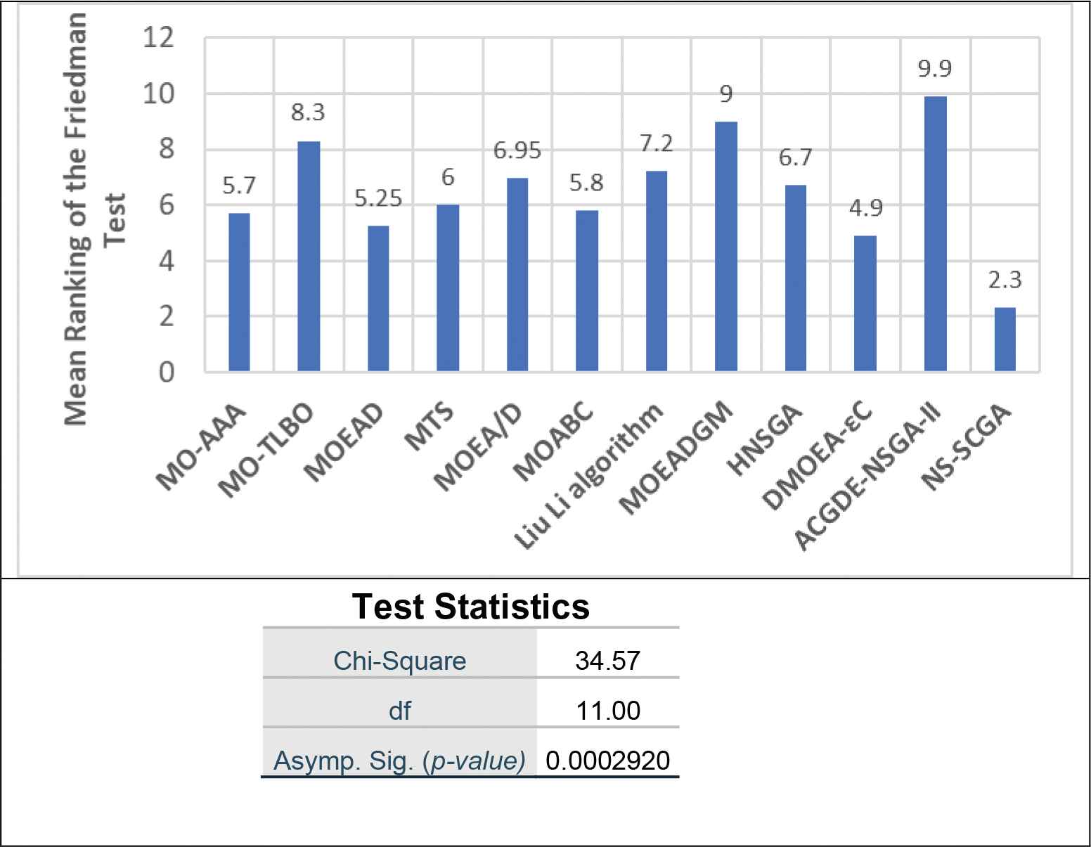
Friedman test on nondominated sorting sine-cosine genetic algorithm (NS-SCGA) and its 11 competitors on all the unconstrained CEC09 benchmark problems in terms of inverted generational distance (IGD).
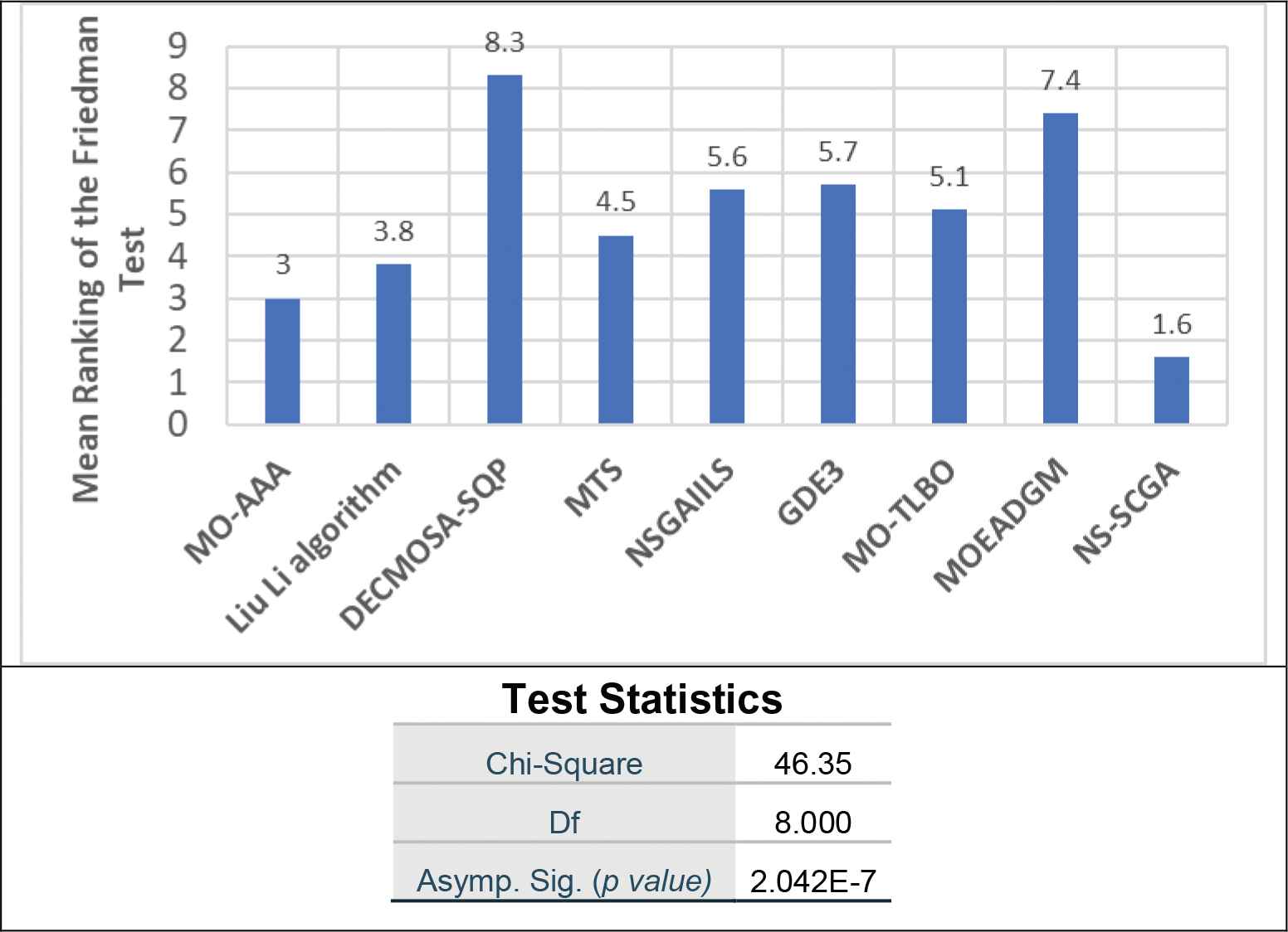
Friedman test on nondominated sorting sine-cosine genetic algorithm (NS-SCGA) and its 8 competitors on all the constrained CEC09 benchmark problems in terms of inverted generational distance (IGD).
In Friedman's test statistics in Figures 8 and 9, there are three values: Chi-Square, df, and Asymp. Sig., where the Chi-Square basically summarizes how differently the algorithms were rated in a single number, while df is the degrees of freedom associated with our test statistic, and finally Asymp. Sig. is the approximate p-value.
As shown in Figures 8 and 9, we can see that the p-value (Asymp. Sig.) is less than the level of significance (Alpha = 5%) in the two cases (unconstrained and constrained problems). This denotes that the algorithms used in the comparison differ in performance. Furthermore, the performance of NS-SCGA is better than the competitors as it has the lowest ranked mean.
According to the Friedman test, it can be concluded that NS-SCGA is an efficient and competitive MO algorithm.
The Wilcoxon signed-rank test
The Wilcoxon signed-rank test was also performed to detect significant differences between the behaviors of the algorithms' pair. Wilcoxon test provides the p-value, that is, the probability that the difference in the performance achieved by the two algorithms is obtained by chance and is not statistically significant [91].
In Tables 6 and 7, NS-SSGA is compared with the other algorithms in terms of IGD in constrained and unconstrained benchmark function, respectively, by applying the Wilcoxon signed-rank test to determine whether NS-SCGA is statistically better than other algorithms or not.
| N | Mean Rank | Sum of Ranks | p-value | ||
|---|---|---|---|---|---|
| NS-SCGA vs MO-AAA | Negative ranks | 9.000 | 5.440 | 49.00 | 0.02800 |
| Positive ranks | 1.000 | 6.000 | 6.000 | ||
| NS-SCGAvs MO-TLBO | Negative ranks | 9.000 | 5.110 | 46.00 | 0.05900 |
| Positive ranks | 1.000 | 9.000 | 9.000 | ||
| NS-SCGAvs MOEA/D | Negative ranks | 8.000 | 5.500 | 44.00 | 0.09300 |
| Positive ranks | 2.000 | 5.500 | 11.00 | ||
| NS-SCGA vs MTS | Negative ranks | 9.000 | 5.000 | 45.00 | 0.07400 |
| Positive ranks | 1.000 | 10.00 | 10.00 | ||
| NS-SCGA vs DMOEADD | Negative ranks | 9.000 | 5.330 | 48.00 | 0.03700 |
| Positive ranks | 1.000 | 7.000 | 7.000 | ||
| NS-SCGA vs MOABC | Negative ranks | 8.000 | 5.130 | 41.00 | 0.1640 |
| Positive ranks | 2.000 | 7.000 | 14.00 | ||
| NS-SCGA vs Liu Li algorithm | Negative ranks | 9.000 | 5.560 | 50.00 | 0.02200 |
| Positive ranks | 1.000 | 5.000 | 5.000 | ||
| NS-SCGA vs MOEADGM | Negative ranks | 10.00 | 5.500 | 55.00 | 0.005000 |
| Positive ranks | 0.000 | .000 | .00 | ||
| NS-SCGA vs HNSGA | Negative ranks | 9.000 | 5.670 | 51.00 | 0.01700 |
| Positive ranks | 1.000 | 4.000 | 4.000 | ||
| NS-SCGA vs DMOEA-εC | Negative ranks | 7.000 | 4.860 | 34.00 | 0.5080 |
| Positive ranks | 3.000 | 7.000 | 21.00 | ||
| NS-SCGA vs ACGDE-NSGAII | Negative ranks | 10.00 | 5.500 | 55.00 | 0.005000 |
| Positive ranks | 0.00 | .00 | .00 | ||
Nondominated sorting sine-cosine genetic algorithm (NS-SCGA) pairwise comparisons: Wilcoxon test summary for the CEC09 unconstrained benchmark functions.
| N | Mean Rank | Sum of Ranks | p-value | ||
|---|---|---|---|---|---|
| NS-SCGA vs MOAAA | Negative ranks | 8.000 | 6.000 | 48.00 | 0.03700 |
| Positive ranks | 2.000 | 3.500 | 7.000 | ||
| NS-SCGA vs Liu Li algorithm | Negative ranks | 8.000 | 5.880 | 47.00 | 0.04700 |
| Positive ranks | 2.000 | 4.000 | 8.000 | ||
| NS-SCGA vs DECMOSA-SQP | Negative ranks | 10.00 | 5.500 | 55.00 | 0.005000 |
| Positive ranks | 0.00 | 0.000 | 0.000 | ||
| NS-SCGA vs MTS | Negative ranks | 9.000 | 5.560 | 50.00 | 0.02200 |
| Positive ranks | 1.000 | 5.000 | 5.000 | ||
| NS-SCGA vs NSGAIILS | Negative ranks | 9.000 | 5.670 | 51.00 | 0.01700 |
| Positive ranks | 1.000 | 4.000 | 4.000 | ||
| NS-SCGA vs GDE3 | Negative ranks | 10.00 | 5.500 | 55.00 | .0.005000 |
| Positive ranks | 0.000 | 0.000 | 0.000 | ||
| NS-SCGA vs MO-TLBO | Negative ranks | 10.00 | 5.500 | 55.00 | 0.005000 |
| Positive ranks | 0.00 | .0000 | 0.00 | ||
| NS-SCGA vs MOEADGM | Negative ranks | 10.00 | 5.500 | 55.00 | 0.005000 |
| Positive ranks | 0 | 0.000 | 0.00 | ||
Nondominated sorting sine-cosine genetic algorithm (NS-SCGA) pairwise comparisons: Wilcoxon test summary for the CEC09 constrained benchmark functions.
As shown in Table 6, the Wilcoxon test results indicate that the NS-SCGA had a better statistically significant performance compared to MO-AAA, DMOEADD, Liu li algorithm, MOEADGM, and ACGDE-NSGAII as p-value is smaller than the level of significance (Alpha = 5%). But there is no statistically significant difference between the NS-SCGA on one hand and MO-TLBO, MOEA/D, MTS, MOABC, and DMOEA-εC on the other hand as p-value is greater than the level of significance (5%).
On the other hand, all p-values of the Wilcoxon test results in Table 7 are less than 5%. Therefore, there are statistically significant differences between NS-SCGA and the other algorithms. NS-SCGA was significantly better than the other algorithms in solving constrained benchmark functions.
In view of the results of Wilcoxon signed-rank test, it can be concluded that the NS-SCGA is superior to most of the compared algorithms in solving MOPs.
6.6. The EEDP: Case Study
The main objective of EEDP is the minimization of fuel cost and emission of atmospheric pollutants which are two conflicting objective functions while satisfying inequality and equality constraints foist by the power system requirements. The objectives and constraints of EEDP are given below [38]:
Objective
The total fuel cost is formulated as a quadratic function in terms of real power output as follows:
and the total emission of atmospheric pollutants from fossil-fueled thermal stations in ton/h can be represented bywhereConstraints
Power balance constraint The total generated power must cover the power demand
Generation capacity constraints Each generator is restricted to generate output real power within the range of the maximum and minimum output power; that is,
where
NS-SCGA has been tested on IEEE 30-bus 6-generator test system for power demand
The IEEE 30-bus 6-generator test system has 21 load buses and 41 transmission lines [92].
The parameters of that test system including fuel cost coefficients, emission coefficients, and the B-coefficients are taken from [93]. The parameter settings which are used for optimizing the EEDP are the following: the size of population Npop = 200 individuals, the maximum number of generations
Figure 10 gives the obtained Pareto-optimal front by NS-SCGA during the best optimization run implementation. This figure shows the tradeoff between fuel cost and emissions. This figure proves that NS-SCGA is capable of obtaining the Pareto-optimal front with good diversity and convergence characteristics.
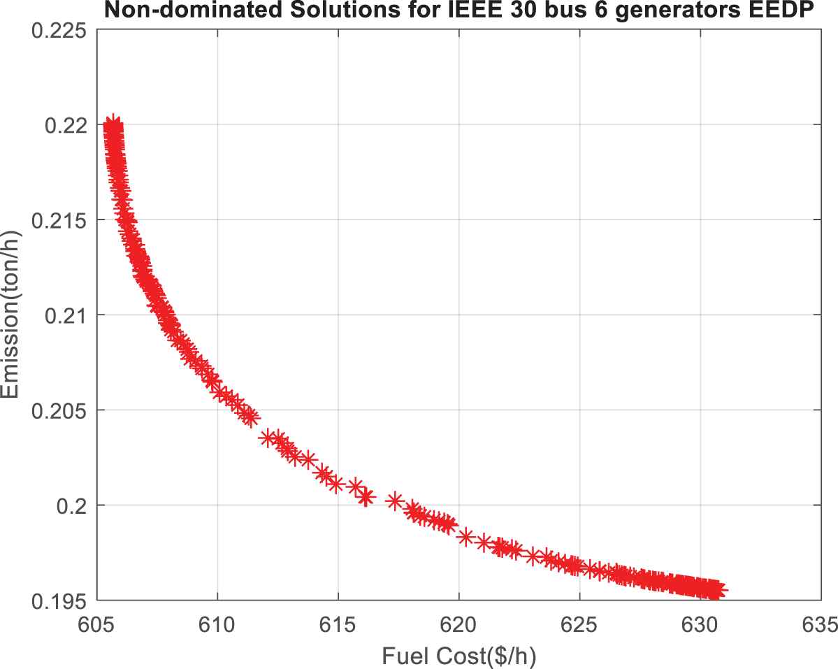
The obtained Pareto front of IEEE 30-bus 6-generator system by nondominated sorting sine-cosine genetic algorithm (NS-SCGA).
The schedules of the generation that give the minimum fuel cost (along with the corresponding emission) obtained by NS-SCGA and the other techniques are presented in Table 8. Similarly, Table 9 gives the schedules of the generation that yield to the minimum emissions. Since the power demand is measured in “p.u.,” the unit of output powers obtained by the proposed algorithm is measured by p.u. Moreover, Table 10 shows the results of the comparison between the three techniques in terms of SP metric.
| NPGA | MO-DE/PSO | MOHS | SPEA | NSGA-II | NSGA-II/EDA | TV-MOPSO | MOCDOA | NS-SCGA | |
|---|---|---|---|---|---|---|---|---|---|
| PG1 | 0.1245 | 0.1220 | 0.06790 | 0.1086 | 0.1119 | 0.1399 | 0.1482 | 0.1204 | 0.1148 |
| PG2 | 0.2792 | 0.2843 | 0.3515 | 0.3056 | 0.3265 | 0.3219 | 0.3062 | 0.2871 | 0.2901 |
| PG3 | 0.6284 | 0.5857 | 0.5174 | 0.5818 | 0.5857 | 0.5597 | 0.5798 | 0.5803 | 0.5742 |
| PG4 | 1.026 | 0.9962 | 0.8839 | 0.9846 | 0.9329 | 0.9487 | 1.000 | 0.9922 | 0.9922 |
| PG5 | 0.4693 | 0.5149 | 0.5991 | 0.5288 | 0.5623 | 0.5254 | 0.4529 | 0.5259 | 0.5241 |
| PG6 | 0.3993 | 0.3566 | 0.4317 | 0.3584 | 0.3404 | 0.3651 | 0.3725 | 0.3537 | 0.3619 |
| Fuel Cost | 608.1 | 606.0 | 606.3 | 607.8 | 606.6 | 606.5 | 606.4 | 606.0 | 605.4 |
| Emission | 0.2236 | 0.2209 | 0.2148 | 0.2202 | 0.2170 | 0.2164 | 0.2198 | 0.2206 | 0.2206 |
| NFEs | 1.000E5 | 1.000E4 | N/a | 1.000E5 | 2.250E4 | 2.250E4 | 2.500E4 | 2.000E4 | 2.000E4 |
Comparison of the best solutions obtained by different algorithms for minimizing the fuel cost.
| SPEA | NPGA | NSGA-II/EDA | NSGA-II | MOHS | MO-DE/PSO | TV-MOPSO | MOCDOA | NS-SCGA | |
|---|---|---|---|---|---|---|---|---|---|
| PG1 | 0.4043 | 0.3923 | 0.4135 | 0.4135 | 0.4937 | 0.4118 | 0.3926 | 0.4103 | 0.3985 |
| PG2 | 0.4525 | 0.4700 | 0.4662 | 0.4663 | 0.3908 | 0.4616 | 0.4724 | 0.4668 | 0.4626 |
| PG3 | 0.5525 | 0.5565 | 0.5483 | 0.5482 | 0.5506 | 0.5435 | 0.5484 | 0.5437 | 0.5514 |
| PG4 | 0.4079 | 0.3695 | 0.3948 | 0.3949 | 0.3774 | 0.3922 | 0.4133 | 0.3901 | 0.4066 |
| PG5 | 0.5468 | 0.5599 | 0.5484 | 0.5483 | 0.5420 | 0.5454 | 0.5503 | 0.5426 | 0.5460 |
| PG6 | 0.5005 | 0.5163 | 0.5187 | 0.5186 | 0.5021 | 0.5148 | 0.4909 | 0.5157 | 0.5025 |
| Emission | 0.1942 | 0.1942 | 0.1942 | 0.1942 | 0.1951 | 0.1942 | 0.1943 | 0.1942 | 0.1941 |
| Fuel Cost | 642.6 | 646.0 | 650.8 | 650.8 | 674.4 | 646.0 | 642.8 | 646.3 | 643.4 |
Comparison of the best solutions obtained by different algorithms for minimizing emissions.
| Algorithm | Spacing |
||
|---|---|---|---|
| Best | Mean | Standard Deviation | |
| NS-SCGA | 0.005500 | 0.005987 | 0.0009411 |
| TV-MOPSO | 0.01080 | 0.01080 | 0.01740 |
| MO-DE/PSO | 0.005100 | 0.007400 | 0.002800 |
SP metric values of the proposed NS-SCGA, TV-MOPSO, and MO-DE/PSO for EEDP.
It is quite evident from Table 8 that the NS-SCGA obtains the minimum fuel cost which is equal to 605.4 $/h (United States dollar/hour) using 2.000E+4 NFEs. Furthermore, the performance of NS-SCGA is better compared to NPGA, MO-DE/PSO, TV-MOPSO, SPEA, MOHS, NSGA-II, NSGA-II/EDA, and MOCDOA in terms of fuel cost. Also, NS-SCGA outperforms NPGA, TV-MOPSO, SPEA, MOHS, NSGA-II, and NSGA-II/EDA in terms of NFEs. MO-DE/PSO returned the lowest value of NFEs which is 1.000E+4 but it obtained fuel cost equal to 606.0 which is more than that obtained by MOCDOA and by the NS-SCGA.
In Table 9, the minimum emission obtained by NS-SCGA is equal to 0.1941 which is almost the same as that obtained by MO-DE/PSO, NSGA-II, and MOCDOA. But the fuel cost corresponding to the minimum emission obtained by NS-SCGA is lower than other algorithms.
In addition, from Table 10 it is quite evident that the performance of NS-NSGA is far better than the other compared algorithms, where the distribution of TV-MOPSO and MO-DE/PSO is not as good as that of NS-SCGA. Moreover, the obtained Pareto front by NS-SCGA shown in Figure 10 further demonstrates the excellent solutions distribution of the obtained Pareto front. As seen from the above results, NS-SCGA is able to obtain high-quality results when compared with the other techniques in solving EEDP of IEEE 30-bus 6-generator system.
6.6.1. Identifying the best compromise solutions from the obtained Pareto front by the TOPSIS technique
In this subsection, the obtained Pareto-optimal solutions, from NS-SCGA, undergo the TOPSIS techniques as a multiattribute decision analyzing technique, to rank the Pareto-optimal solutions according to the preference of DM and identifying the best compromise solutions. The principle of TOPSIS is based on obtaining the best compromise solution which is the farthest from the negative ideal solution (nis) and closest to the positive ideal solution (pis). The computational steps of TOPSIS technique which are applied to Pareto-optimal solutions of EEDP are as follows [68]:
Input the objective matrix OM = (OMnm), whose elements are the Pareto solutions. Each row of the objective matrix is allocated to one alternative and each column to one objective. Therefore, the element OMnm of the objective matrix is the mth objective value of the nth optimal solution, where
Input as well a weight vector
Normalize the OM to be normalized objective matrix NOR = (NORnm) using the equation below to be the normalized value NORnm
As follows:
where NORnm is the normalized rating; OMnmis the mth objective value of the nth optimal solution.Determine the weighted normalized objective matrix WN = (WNnm), and the weighted normalized value WNnm is calculated by
Calculate nis and pis individually as follows:
whereCalculate the separation measure sep and sn from the pis and nis, respectively:
Calculate the relative closeness
Identify the best compromise solution which has relative closeness
The above steps are applied to the obtained Pareto-optimal solutions by NS-SCGA. w1 and w2 represent the DM's preference of each objective, where w1 is the weight of fuel cost (i.e., the relative importance of the fuel cost) and w2 is the weight of emission (i.e., the relative importance of the emission).
In order to study the effect of changing the weights on the fuel cost and emission, the weight of fuel cost is assumed w1 = 0, 0.1, 0.2, 0.3, 0.4, 0.5, 0.6, 0.7, 0.8, 0.9, 1, and the weight of emission is obtained by
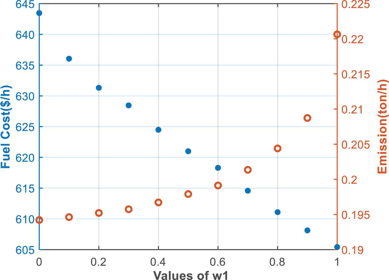
The best compromise solutions in the objective space according to w1.
| w1 | Fuel cost | Emission | PG1 | PG2 | PG3 | PG4 | PG5 | PG6 |
|---|---|---|---|---|---|---|---|---|
| 0 | 643.5 | 0.1942 | 0.3985 | 0.4626 | 0.5514 | 0.4066 | 0.5460 | 0.5025 |
| 0.1 | 636.0 | 0.1946 | 0.3690 | 0.4441 | 0.5544 | 0.4664 | 0.5445 | 0.4867 |
| 0.2 | 631.3 | 0.1952 | 0.3490 | 0.4303 | 0.5505 | 0.5108 | 0.5425 | 0.4806 |
| 0.3 | 628.5 | 0.1957 | 0.3377 | 0.4211 | 0.5486 | 0.5373 | 0.5509 | 0.4672 |
| 0.4 | 624.5 | 0.1967 | 0.3149 | 0.4086 | 0.5618 | 0.5761 | 0.5407 | 0.4594 |
| 0.5 | 621.0 | 0.1979 | 0.2960 | 0.3967 | 0.5602 | 0.6174 | 0.5405 | 0.4497 |
| 0.6 | 618.3 | 0.1991 | 0.2821 | 0.3857 | 0.5561 | 0.6490 | 0.5587 | 0.4279 |
| 0.7 | 614.6 | 0.2013 | 0.2471 | 0.3839 | 0.5569 | 0.7007 | 0.5585 | 0.4112 |
| 0.8 | 611.1 | 0.2044 | 0.2233 | 0.3558 | 0.56290 | 0.7685 | 0.5322 | 0.4149 |
| 0.9 | 608.1 | 0.2087 | 0.1958 | 0.3329 | 0.5662 | 0.8424 | 0.5290 | 0.3908 |
| 1.0 | 605.4 | 0.2206 | 0.1148 | 0.2901 | 0.5742 | 0.9922 | 0.5241 | 0.3619 |
The best compromise solutions for fuel cost and emission according to w1.
7. CONCLUSIONS
A new MO algorithm called NS-SCGA is presented in this paper. The NS-SCGA is tested on 20 challenging benchmark problems from CEC09 for UCMOPs and CMOPs and its performance is calculated by IGD, spacing, and spreading metrics. NS-SCGA has been compared with another 11 newly developed algorithms and another 8 recent algorithms for unconstrained problems and constrained problems, respectively. The LO is used to assess the overall performance of the proposed NS-SCGA among the compared techniques. The statistical analysis of the experimental results is also carried out by nonparametric Friedman and Wilcoxon signed-rank tests. In addition, NS-SCGA has been applied to handle EEDP. The EEDP is formulated as a MOP with two conflicting objectives, that is, cost and emission. NS-SCGA has been validated on the IEEE 30-bus 6-generator system. The obtained results by the NS-SCGA have been compared with other metaheuristic algorithms. It is evident from the comparison that the NS-SCGA gives a competitive performance in terms of solution. Finally, the TOPSIS method is used to identify the best compromise solution from the obtained nondominated solutions of EEDP according to the DM's preference.
The results prove that NS-SCGA is better or on a par with the other modern methods for solving MOPs. It is robust, efficient, and simple, and it has the possibility of being applied to solve some other MO power system problems.
CONFLICT OF INTEREST
The authors declare no conflict of interest.
AUTHORS’ CONTRIBUTIONS
All authors are equally contributed in this article.
Funding Statement
The authors received no specific funding for this work.
ACKNOWLEDGMENTS
The authors would like to thank the referees for valuable remarks and suggestions that helped to increase the clarity of arguments and to improve the structure of the paper. In addition, thanks are due to Mr. Muhammad Anwar (muhammad.anwar.hashim@gmail.com), MA student in linguistics and English instructor at German University in Cairo, for English-language editing.
REFERENCES
Cite this article
TY  - JOUR
AU  - M.A. Farag
AU  - M.A. El-Shorbagy
AU  - A.A. Mousa
AU  - I.M. El-Desoky
PY  - 2020
DA  - 2020/06/29
TI  - A New Hybrid Metaheuristic Algorithm for Multiobjective Optimization Problems
JO  - International Journal of Computational Intelligence Systems
SP  - 920
EP  - 940
VL  - 13
IS  - 1
SN  - 1875-6883
UR  - https://doi.org/10.2991/ijcis.d.200618.001
DO  - 10.2991/ijcis.d.200618.001
ID  - Farag2020
ER  -