
Automated Recognition of Hand Grasps Using Electromyography Signal Based on LWT and DTCWT of Wavelet Energy
 , S. Mary Vasanthi2, T. Jayasree3
- DOI
- 10.2991/ijcis.d.200724.001How to use a DOI?
- Keywords
- Signal processing; Electromyogram; Discrete wavelet transform; Feature extraction; Pattern recognition; Support vector machine; Deep Learning Neural Network
- Abstract
This paper presents a novel framework that automatically classifies hand grasps using Electromyogram (EMG) signals based on advanced Wavelet Transform (WT). This method is motivated by the observation that there lies a unique correlation between different samples of the signal at various frequency levels obtained by Discrete WT. In the proposed approach, EMG signals captured from the subjects are subjected to denoising using symlet wavelets, followed by Principal Component Analysis (PCA) for dimensionality reduction. Further, the important attributes of the signal are extracted using Lifting Wavelet Transform (LWT) and Dual Tree Complex WT (DTCWT). Multiple classifiers such as Feed Forward Neural Networks (FFNN), Cascaded Feed Forward Neural Networks (CFNN), Support Vector Machine (SVM) and Deep Learning Neural Network (DLNN) are used for classification. The simulation results are compared with various training algorithms and it is observed that DTCWT features combined with CFNN and trained with Gradient Descent with Adaptive Back Propagation (GDABP) algorithm achieved the best performance. The advantages of the proposed method were proved by comparing with the earlier conventional methods, in terms of recognition performance. These experimental results prove that the proposed method gives a potential performance in the recognition of hand grasps using EMG signals. In addition, the proposed method supports clinicians to improve the performance of myoelectric pattern recognition.
- Copyright
- © 2020 The Authors. Published by Atlantis Press B.V.
- Open Access
- This is an open access article distributed under the CC BY-NC 4.0 license (http://creativecommons.org/licenses/by-nc/4.0/).
1. INTRODUCTION
Electromyogram (EMG) signals are the bio-signals, which vary with time and are recorded from the muscles by the insertion of electrodes [1,2]. An EMG signal consists of rich neural information relating to hand movements and their functionality and hence is effectively applied for prosthesis [3,4], rehabilitation systems or in the diagnosis of neuromuscular diseases [5,6].
The EMG signals are greatly contaminated with background noises and other signals, while traversing through different tissues. Moreover, Motor Unit Action Potentials (MUAPs) are added to various noisy signals during signal retrieval. Thus, the EMG signal gets distorted seriously due to the addition of noise during acquisition and recording process. Due to these reasons, the EMG signal becomes very complex and it needs to be denoised. A 50Hz notch filter was included to process the acquired raw signal [7]. To remove power-line interferences, movement artifacts and high-frequency noises, a 5Hz, zero phase, second order, low-pass Butterworth filter was used [8]. Preprocessing of surface EMG (sEMG) signals can be done by whitening and spatial filtering to enhance pattern recognition accuracies [9,10].
2. RELATED WORK
This section reviews some of the recent works on hand grasp classification using Machine-learning and Support Vector Machine (SVM) techniques.
Various Time-Domain (TD) features were extracted from the EMG signals for further analysis. Researchers [11,12], investigated the performance of different TD features for recognizing five hand gestures. Khushaba et al. [13], proposed TD feature set with SVM classifier for the recognition of hand grasps at various contraction levels with different forearm orientations. In fact, TD features in EMG analysis have to be carefully assessed in order to reduce the time delay. Mesa et al. [14] used frequency domain based features and cepstral coefficients together with SVM classifier for classifying different hand gestures. But these feature sets are not optimum regardless of the gestures. Khushaba et al. [15] proposed frequency domain based features such as moments and spectral flux together with Linear Discriminant Analysis (LDA) classifier for classifying eight different classes of hand movements. But this method required more computational time.
Wavelet Transform is an effective mathematical time-frequency tool which has been applied to extract the features from the EMG signal [16,17]. In this paper, Discrete Wavelet Transform (DWT) is used for extracting different features from the EMG signal. The nonlinear properties of the signal can be estimated by finding energy and entropies and most relevant features are selected from the energy distribution characteristics [18].
The development of myoelectric prosthesis control system relies on classification of EMG signals [19,20]. The classification of EMG signals is very tough since there are lots of fluctuations and interferences in the EMG signal [21]. Different types of classifiers include nearest neighbor classifiers, LDA, SVM and Artificial Neural Network (ANN) classifiers [22,23]. ANN is used for the classification of different hand gestures [24,25]. Gokgoz and Subasi [26], proposed the combination of DWT and Decision Tree Algorithm for classifying biomedical signals and Alomari and Liu [27], introduced a pattern recognition system for classifying eight different hand grasps using the energy of wavelet coefficients. ANN was trained using information on the muscle contraction level and prior classifier outputs to understand the reliability of the classifier's decision. Amsuss et al. [28], Guo et al. [29] used ANN to classify six different types of hand gestures with high accuracy but not robust with electrode size, electrode shift and orientation on amputees. Deep Learning Neural Network (DLNN) is an effective machine-learning tool used in computer vision, natural language processing, pattern and speech recognitions [30–34]. It is also used in the classification of brain magnetic resonance imagings (MRIs) into normal or malignant [35]. SVM classifier is very popular because of its robust mathematical theory. It classifies highly nonlinear data due to its powerful learning ability [36,37]. Its quadratic optimization task significantly reduces the number of operations in the learning mode [38,39].
In this paper, Wavelet-based denoising techniques are proposed for the elimination of noises embedded in the EMG signal. Time-frequency domain (TFD)-based features derived using Lifting Wavelet Transform (LWT) and Dual Tree Complex wavelet transform (DTCWT) are used to characterize the EMG signals in the classification of hand grasps. It has been observed that these features are different for various hand grasps and they can be used as input for Feed Forward Neural Networks (FFNN), Cascaded Feed Forward Neural Networks (CFNN), DLNN and SVM classifiers which can classify various hand grasps [40].
The paper is organized as follows: The next section presents the methodology of the proposed framework. Section 4 provides data acquisition procedure and preprocessing. Section 5 details the extraction of LWT- and DTCWT-based features. In Section 6, methods involved in each step of EMG signal classification have been introduced. It also gives a detailed experimental study of classification using feed forward pattern recognition network models and SVM. Results and Discussion are presented in Section 7. Finally, Section 8 summarizes the conclusions.
3. METHODOLOGY
The proposed framework for automated hand grasp recognition involves three different stages: Data acquisition and preprocessing, feature extraction and classification system as shown in Figure 1. First, the EMG signals of the forearm muscles are detected and captured by sensors and further preprocessed to remove the movement artifacts and power-line interferences. The recorded signals are the discrete samples of size between 10000 and 20000 for a typical motion. But, this primary representation of the signals in terms of samples hinders the classification and thus it requires dimensionality reduction. This reduction helps to represent the signal as a feature vector. Feature extraction from the original EMG signal is achieved through transformation in the time–frequency domain by the decomposition of signal into signal components at different frequencies and finding energy characteristics. ANN-based classification is a machine-learning process that deals with the recognition of patterns and regularities in data. The algorithm may be statistical or nonstatistical in nature and depends on whether the learning is supervised or unsupervised.
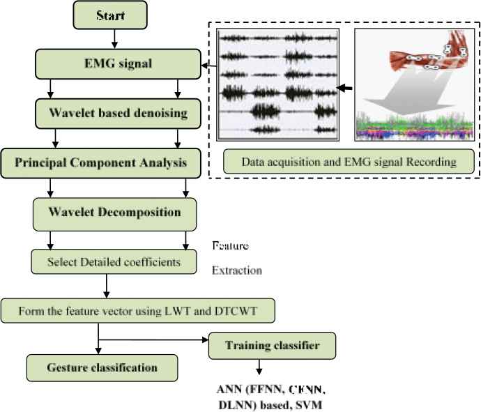
Electromyogram-based hand grasp recognition system.
4. DATA ACQUISITION AND PREPROCESSING
Eight subjects, five males and three females, aged between 19 and 22, free of any muscular/neurological disorders volunteered to perform the experiment. Subjects were asked to be seated in an armchair, with their arm fixed at one end so that they could perform hand postures without any constraints as shown in Figure 2. The EMG data was collected using Ag/AgCl disposable surface electrodes which were positioned at equidistance on the subject's right forearm.
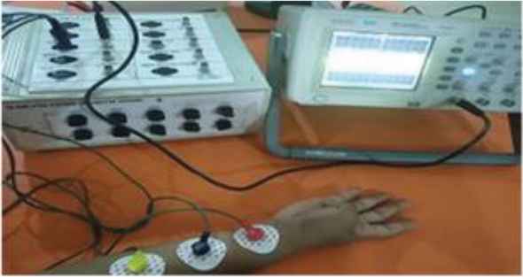
Experimental setup.
For the experiment, 6 different hand grasps namely Palmar Class (PC), Spherical Class (SC), Hook Class (HC), Cylindrical Class (CC), Tip Class (TC) and Lateral Class (LC) were selected and they are shown in Figure 3. The subjects were requested to perform each grasp in 2 trials and recorded for 3 sec.
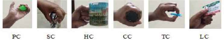
Different hand grasps.
4.1. Wavelet Denoising
For the removal of noise present in the EMG signal, wavelet denoising is performed. In wavelet denoising, some of the signal details represent the average power of the signal and the other represents the noise value. Hence, if the details representing the noise are filtered, the signal can be reconstructed again using other details, without any loss of information present in the signal. Thus, it is necessary to select suitable threshold algorithm and scaling function. Let us suppose the signal
The steps involved in the recovery of original signal x(t) are summarized below:
Perform wavelet decomposition of
Apply the nonlinear soft thresholding operator to the noisy wavelet coefficients given by
Find the Inverse and estimate the signal from the new coefficients
The signal is thresholded using
Where L denotes the number of decomposition levels.
The detailed block diagram description of wavelet denoising is shown in Figure 4.
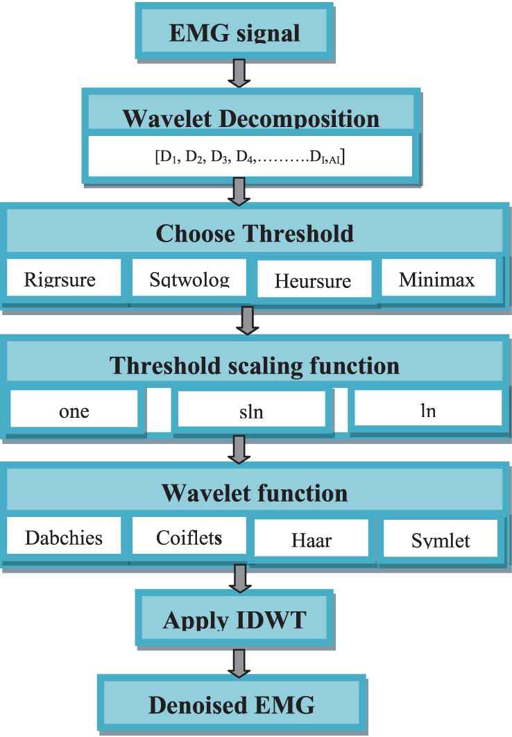
Block diagram for wavelet denoising.
Four different thresholding techniques (1) Rigrsure (2) Sqtwolog (3) Heursure and (4) Minimaxi are applied to the wavelet coefficients of the EMG signal. Proper thresholding is done by selecting the threshold functions (one, sln, ln) and wavelet functions (db, coif, haar, sym).
4.2. Principal Component Analysis
Principal Component Analysis (PCA) is employed to reduce the dimensions of the data sets. Using PCA, an n-dimensional data is represented in a lower dimensional space. It is useful for segmenting signals from multiple sources. A small number of uncorrelated principal components were derived from a larger set of zero-mean variables, un altering the maximum possible amount of information from the original data. Principal components are computed, which are the basis vectors of directions in decreasing order of variability. The first principal component gives the basis vector for the direction of highest variability. The second principal component provides the basis vector for the next direction orthogonal to the first principal component and so on. A percentage of total variability of the data is set as the threshold in order to select the number of principal components. Computation of principal components involves calculating the covariance matrix of the data, decomposition of its eigen value, sorting of eigenvectors in the decreasing order of eigen values and finally projecting the data into the new basis defined by principal components by calculating the inner product of the original signals and the sorted eigenvectors.
5. FEATURE EXTRACTION
In the pattern recognition problems, the dimensionality of the input is desired to keep it as small as possible in order to obtain higher classification accuracy and lower computation time. Suppose EMG signal from one channel can be denoted as a finite series
5.1. Lifting Wavelet Transform
This is a more effective method of implementing wavelet transform. A lifting algorithm includes three steps namely split, predict and update for signal decomposition.
Split: The input signal S is splitted into an even signal
Predict: The even signal
Update: The data
The LWT reduces computation time and enables frequency localization to overcome the drawbacks of the traditional wavelets.
5.2. Dual Tree Complex Wavelet Transform
Some of the drawbacks of DWT such as shift sensitivity, absence of phase information and poor directionality are overcome by DTCWT. It is a form of DWT with dual-tree approach having two DWTs or trees (i) Tree a (first DWT) gives the real part of the transform and (ii) Tree b (second DWT) gives the imaginary part. A pair of low-pass and high-pass filters are used for tree a and tree b with wavelet function
The low frequency filter coefficients or approximations are given by
The high-frequency filter coefficients or details are given by
Using these filters, the DTCWT simultaneously decomposes the input signals to obtain approximation and detail coefficients at real (tree a) and imaginary (tree b) parts. Thus, two approximation (real and imaginary) and two detail coefficients (real and imaginary) are obtained at each level of decomposition.
5.3. Energy Distribution
The energy of the EMG signal can be distributed at different resolution levels in different ways depending on the hand grasp. The coefficient of detailed version at each decomposition level is used to retrieve features from the signal to enable classification of different hand grasps. The energy of the signal can be expressed mathematically by
The normalized energy is
Algorithm for wavelet-based Energy:
Data: S = (signal, sampling freq) recorded emg signal
Result: Energy
begin
for signal S do
1. Set the wavelet decomposition level, n = 1, 2,……‥ N
2. Decompose into Approximations and Details
3. Select the detailed coefficients {D, DD, DDD……‥}
end
for n Detailed coefficients
Find Energy at each decomposition level {ED, EDD, EDDD……}.
The feature set was computed for two channels and then grouped to form an n-dimensional feature vector, where n denotes number of decomposition levels. Thus, for the resolution level 4, 16-dimensional feature vectors are obtained and for level 5, 32-dimensional feature vectors are obtained.
6. CLASSIFICATION METHODS
The features were classified using multiple classifiers such as FFNN, CFNN, SVM and DLNN and their classification accuracies were compared.
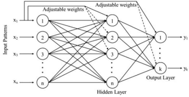
6.1. ANN-Based Pattern Recognition System
Multilayer FFNN is used for recognizing the hand grasps. The hidden units compute their activation and send signals to the output units. The value associated with the connection path between input layer neurons and hidden layer neurons is known as input-hidden layer weight and that of between hidden layer neurons and output layer neurons is known as hidden-output layer weight. The input and output of node j is computed as
The weights are updated to minimize the mean squared error.
ANNs were trained and tested using Gradient Descent Back Propagation (GDBP), Levenberg-Marquardt Back Propagation (LMBP), Gradient descent with Adaptive Back Propagation (GDABP), Gradient Descent with Momentum Back Propagation (GDMBP) and Gradient Descent with Momentum and Adaptive Back Propagation (GDMABP) training algorithms and their performances were analysed.
GDBP: A set of parameters θ = {w, b} was determined after training a neural network to minimize the errors that occur in the network. The choice of the error function εi is the sum of the squared difference between the target tk and the network output ak. This problem can be solved using gradient descent, which requires determining
LMBP: The performance function of this algorithm is represented in terms of the sum of squares. This algorithm uses Hessian matrix, given by
GDABP: It first determines the output of initial network and the corresponding error. New weights and biases are obtained at each iteration using the present learning rate. Again, new outputs and errors are obtained. If the new error is above the previous one by more than a predefined value, the new weights and biases are rejected and the learning rate is reduced. Otherwise, the new weights are accepted. If the present error is smaller than the previous error, the learning rate is increased.
GDMBP: The weights of the network are updated along the negative gradient of the performance function. Moreover, this algorithm makes use of momentum, which allows the network to respond to the local gradient and also to recent trends in the error surface, thus allowing the network to avoid getting struck into local minima.
GDMABP: It updates weight and bias values using gradient descent momentum and an adaptive learning rate. The algorithm trains any network as long as its transfer functions, weight and net input have derivative functions.
6.2. CFNN-Based Classification
Pattern recognition is a process of comprehending a pattern of a given object based on the knowledge already possessed. The performance of CFNN depends on Hessian matrix given by
Cascaded Feed Forward Neural Network [41].
The main steps of the learning CFNN algorithm are described below:
Step 1: Select the required input and output units and train the net until error reaches a minimum value.
Step 2: Compute the residual error,
Step 3: Add first hidden unit.
Step 4: A candidate unit X is connected to each input unit (not connected to the output units) and initialize weights from input units to X. These weights are trained to maximize correlation C.
whereStep 5: Train all the weights w of the output units. If acceptable error has been reached, stop. Otherwise go to step 6.
Step 6: If stopping condition is false, do steps 7 and 8.
Step 7: A candidate unit X is connected to each input unit and each previously added hidden unit. These weights are trained to maximize C.
Step 8: Train all the weights w to the output units. If acceptable error has been reached, stop; else, repeat the above procedure.
6.3. DLNN-Based Classification
DLNN algorithms attempt to learn multiple levels of representation using a hierarchy of multiple layers and the learned features are able to adapt. The main steps of the learning DLNN algorithm are described below:
Step 1: Randomly initialize the weights of the network.
Step 2: Apply gradient descent using back propagation network.
Step 3: Sample the labeled data called batch.
Step 4: Samples are forwarded through the network to get predictions.
Step 5: An error signal is generated which is the difference between predictions and target values.
Step 6: These errors are back propagated to update the weights and to get more accurate predictions.
Step 7: Subtract a fraction of the gradient to get the local minimum of the cost function.
6.4. SVM-Based Classification
The steps involved in SVM algorithm are given below:
Step 1: Let xi be a vector of length m and each belong to one of two classes labeled as “+1” and “−1.”
Step 2: Let the training set be
Step 3: Let the separating hyper plane be w.
Step 4: Support vectors are the samples nearer to the separating hyper plane. The separating hyper plane equation is
x ϵ Rm, b ϵ R.
7. RESULTS AND DISCUSSIONS
The EMG data are collected from different subjects as discussed in Section 3. Totally 30,000 data samples could be acquired during each hand grasp. While capturing the signal, there may be possibilities of adding noises due to the placement of sensors and other background noises with the EMG signal. Hence, the signal is preprocessed by applying denoising techniques as discussed in Section 3 and the performances were analysed by finding the signal to Interference ratio (SIR).
| Gestures | SIR |
|||||||||||
|---|---|---|---|---|---|---|---|---|---|---|---|---|
| db4 |
coif5 |
sym4 |
||||||||||
| rigrsure | Heur sure | sqtwolog | Mini maxi | rigrsure | Heur sure | sqtwolog | Mini maxi | rigrsure | Heur sure | sqtwolog | mini maxi | |
| CC1 | 1.0483 | 1.0159 | 1.0116 | 1.0230 | 1.0358 | 1.0000 | 1.0000 | 1.0177 | 1.0277 | 1.0000 | 1.0000 | 1.0069 |
| CC2 | 2.5346 | 2.3129 | 1.1015 | 1.2719 | 2.6552 | 2.5775 | 1.1112 | 1.2725 | 2.5370 | 2.4003 | 1.1096 | 1.2852 |
| CC3 | 1.0949 | 0.9998 | 0.9998 | 1.0141 | 1.0901 | 1.0132 | 1.0080 | 1.0319 | 1.1120 | 1.0131 | 1.0079 | 1.0306 |
| CC4 | 1.2521 | 1.0883 | 1.1031 | 1.1503 | 1.2409 | 1.1163 | 1.1100 | 1.1537 | 1.2487 | 1.1242 | 1.1128 | 1.1521 |
| CC5 | 1.0003 | 1.0003 | 1.0003 | 1.0003 | 1.0001 | 1.0001 | 1.0001 | 1.0001 | 0.9994 | 0.9994 | 0.9994 | 0.9994 |
| CC6 | 2.1006 | 2.0056 | 1.0757 | 1.2145 | 1.9803 | 1.9066 | 1.0844 | 1.2111 | 1.8419 | 1.8321 | 1.0960 | 1.2209 |
| TC1 | 1.0425 | 1.0001 | 0.9999 | 1.0153 | 1.0574 | 1.0000 | 1.0000 | 1.0141 | 1.0664 | 1.0001 | 1.0000 | 1.0262 |
| TC2 | 1.0625 | 1.0120 | 1.0098 | 1.0329 | 1.1133 | 1.0148 | 1.0123 | 1.0405 | 1.1050 | 1.0170 | 1.0153 | 1.0398 |
| TC3 | 1.0819 | 1.0530 | 1.0503 | 1.0545 | 1.1101 | 1.0520 | 1.0501 | 1.0625 | 1.0959 | 1.0595 | 1.0587 | 1.0789 |
| TC4 | 1.0105 | 0.9998 | 0.9998 | 1.0074 | 1.0199 | 1.0000 | 1.0000 | 1.0086 | 1.0308 | 1.0000 | 1.0000 | 1.0087 |
| TC5 | 1.0190 | 0.9999 | 0.9999 | 1.0049 | 1.0090 | 1.0000 | 1.0000 | 1.0034 | 1.0057 | 1.0000 | 1.0000 | 1.0010 |
| TC6 | 1.0010 | 1.0003 | 1.0020 | 1.0000 | 1.0003 | 1.0034 | 1.0112 | 1.0003 | 0.9998 | 0.9998 | 1.0121 | 0.9998 |
| HC1 | 1.0867 | 0.9998 | 0.9997 | 1.0225 | 1.0709 | 1.0046 | 1.0035 | 1.0226 | 1.1042 | 1.0059 | 1.0049 | 1.0218 |
| HC2 | 1.0165 | 1.0044 | 1.0013 | 1.0078 | 1.0085 | 1.0061 | 1.0033 | 1.0093 | 1.0228 | 1.0042 | 1.0011 | 1.0079 |
| HC3 | 1.0948 | 1.0000 | 1.0000 | 1.0118 | 1.1025 | 1.0019 | 1.0000 | 1.0217 | 1.1051 | 1.0000 | 1.0000 | 1.0391 |
| HC4 | 1.1940 | 1.0370 | 1.0186 | 1.1038 | 1.2346 | 1.0545 | 1.0374 | 1.1083 | 1.2448 | 1.0572 | 1.0449 | 1.1058 |
| HC5 | 1.1028 | 1.0000 | 1.0000 | 1.0002 | 1.0778 | 0.9999 | 0.9999 | 1.0135 | 1.0732 | 1.0004 | 0.9999 | 1.0200 |
| HC6 | 1.1468 | 1.0305 | 1.0232 | 1.0730 | 1.2175 | 1.0297 | 1.0229 | 1.0649 | 1.1448 | 1.0256 | 1.0213 | 1.0650 |
| PC1 | 1.0040 | 0.9999 | 0.9999 | 1.0018 | 1.0028 | 1.0000 | 1.0000 | 1.0007 | 1.0050 | 1.0000 | 1.0000 | 1.0024 |
| PC2 | 1.0001 | 1.0001 | 1.0001 | 1.0001 | 1.0242 | 0.9999 | 0.9999 | 0.9999 | 1.0296 | 1.0002 | 1.0002 | 1.0002 |
| PC3 | 1.0090 | 0.9999 | 0.9999 | 1.0027 | 1.0175 | 1.0000 | 1.0000 | 1.0040 | 1.0330 | 0.9999 | 0.9999 | 1.0054 |
| PC4 | 1.0169 | 0.9998 | 0.9998 | 1.0104 | 1.0171 | 0.9998 | 0.9998 | 1.0086 | 1.0332 | 1.0001 | 1.0001 | 1.0125 |
| PC5 | 1.0492 | 1.0006 | 0.9999 | 1.0176 | 1.0750 | 1.0006 | 1.0000 | 1.0177 | 1.0543 | 1.0036 | 1.0005 | 1.0200 |
| PC6 | 1.0139 | 1.0036 | 1.0006 | 1.0091 | 1.0091 | 1.0027 | 1.0000 | 1.0085 | 1.0160 | 1.0010 | 1.0000 | 1.0072 |
| SC1 | 0.9999 | 0.9999 | 0.9999 | 0.9999 | 1.0119 | 1.0000 | 1.0000 | 1.0042 | 1.0063 | 0.9999 | 0.9999 | 1.0000 |
| SC2 | 1.1623 | 1.0465 | 1.0413 | 1.0844 | 1.1536 | 1.0468 | 1.0397 | 1.0834 | 1.1714 | 1.0455 | 1.0416 | 1.0783 |
| SC3 | 1.0161 | 1.0025 | 0.9999 | 1.0138 | 1.0322 | 1.0009 | 1.0000 | 1.0070 | 1.0274 | 1.0000 | 1.0000 | 1.0037 |
| SC4 | 1.3632 | 1.0401 | 1.0280 | 1.1048 | 1.3037 | 1.0512 | 1.0407 | 1.1137 | 1.3493 | 1.0522 | 1.0401 | 1.1117 |
| SC5 | 1.5611 | 1.0527 | 1.0413 | 1.1369 | 1.5612 | 1.0607 | 1.0434 | 1.1467 | 1.5443 | 1.0679 | 1.0520 | 1.1540 |
| SC6 | 1.7765 | 1.2480 | 1.0473 | 1.1664 | 1.7416 | 1.2557 | 1.0558 | 1.1735 | 1.8144 | 1.2563 | 1.0560 | 1.1685 |
| LC1 | 1.0150 | 1.0000 | 1.0000 | 1.0071 | 1.0237 | 1.0308 | 1.0000 | 1.0121 | 1.0249 | 0.9999 | 0.9999 | 1.0109 |
| LC2 | 1.0123 | 0.9999 | 0.9999 | 1.0062 | 1.0257 | 1.0021 | 1.0000 | 1.0122 | 1.0309 | 1.0047 | 1.0028 | 1.0152 |
| LC3 | 1.0036 | 1.0001 | 1.0001 | 1.0001 | 1.0053 | 1.0000 | 1.0000 | 1.0018 | 1.0102 | 0.9999 | 0.9999 | 1.0001 |
| LC4 | 1.0013 | 1.0021 | 1.0213 | 1.0013 | 0.9982 | 0.9989 | 0.9982 | 0.0423 | 0.9997 | 0.9997 | 1.0201 | 1.1520 |
| LC5 | 0.9993 | 0.9993 | 1.0023 | 1.0401 | 1.0003 | 1.0027 | 1.0927 | 1.0003 | 1.0801 | 1.0031 | 1.0003 | 1.0211 |
| LC6 | 0.9996 | 0.9982 | 0.9628 | 0.9996 | 1.0000 | 1.0201 | 1.0000 | 1.0000 | 1.0056 | 0.9998 | 0.9998 | 1.0004 |
| HR | 30 | - | 2 | 2 | 29 | 3 | 2 | 1 | 34 | - | - | 1 |
| (88%) | (6%) | (6%) | (82%) | (9%) | (6%) | (3%) | (97%) | (3%) | ||||
| OV | 6 | - | - | - | 8 | 2 | 2 | - | 16 | - | - | 1 |
| (17%) | (23%) | (6%) | (6%) | (45%) | (3%) | |||||||
CC, cylindrical class; HC, hook class; LC, lateral class; PC, palmar class; SC, spherical class; SIR, signal to interference ratio; TC, tip class.
HR: Hit ratio between in between thresholding rules in numbers (%), OV: Overall hit ratio between wavelets in numbers (%).
Comparison results of SIR using different types of denoising.
For dimensionality reduction, PCA is performed. LWT- and DTCWT-based features were extracted from EMG signals. The back propagation neural networks such as FFNN, CFNN, DLNN and SVM with 5 different types of training algorithm were used to classify 6 types of hand grasps. The samples were divided into 3 sets: 70% for training, 15% for validation and 15% for testing.
Three wavelet functions and four soft thresholding rules were considered for analysing the performance of denoised EMG signals.
In Table 1, bold letters denote the best value between thresholding rules of single wavelet and Italic bold letters denote the best value in between all the wavelets. SIR performance on denoised EMG signals allows finding out the best thresholding rules over the other thresholding rules. It is found that “sym4” wavelet function gives the best SIR rate while comparing with the other two wavelet functions. “rigrsure” gives the best results in “sym4” wavelets. The classifiers were trained using different training algorithms and the classification accuracy obtained and the time elapsed for training are shown in Tables 2 and 3.
| Training Algorithm | Classification Accuracy Using Multiple Classifiers |
Time Elapsed for Training (sec) | |||
|---|---|---|---|---|---|
| FFNN | CFNN | DLNN | SVM | ||
| GDBP | 86.14 | 85.26 | 89.91 | 82.93 | 3.928175 |
| LMBP | 83.26 | 87.64 | 89.54 | 83.48 | 4.735437 |
| GDABP | 84.15 | 98.80 | 92.76 | 84.15 | 2.898825 |
| GDMBP | 83.81 | 87.47 | 88.73 | 83.26 | 3.128672 |
| GDMABP | 85.86 | 89.36 | 89.76 | 82.93 | 5.024105 |
CFNN, Cascaded Feed Forward Neural Networks; DLNN, Deep Learning Neural Network; DTCWT, Dual Tree Complex Wavelet Transform; FFNN, Feed Forward Neural Networks; GDABP, gradient descent with adaptive back propagation; GDBP, gradient descent back propagation; GDMABP, gradient descent with momentum and adaptive back propagation; GDMBP, gradient descent with momentum back propagation; LMBP, Levenberg-Marquardt back propagation; SVM, support vector machine.
Comparison of different training algorithms using DTCWT and multiple classifiers.
| Training Algorithm | Classification Accuracy Using Multiple Classifiers |
Time Elapsed for Training (sec) | |||
|---|---|---|---|---|---|
| FFNN | CFNN | DLNN | SVM | ||
| GDBP | 85.95 | 93.47 | 86.95 | 86.28 | 4.508146 |
| LMBP | 83.63 | 81.64 | 86.17 | 88.27 | 2.609061 |
| GDABP | 84.85 | 96.80 | 83.19 | 86.73 | 2.758885 |
| GDMBP | 85.18 | 90.93 | 97.76 | 86.95 | 2.363004 |
| GDMABP | 83.41 | 92.92 | 85.07 | 86.28 | 2.973394 |
CFNN, Cascaded Feed Forward Neural Networks; DLNN, Deep Learning Neural Network; FFNN, Feed Forward Neural Networks; GDABP, gradient descent with adaptive back propagation; GDBP, gradient descent back propagation; GDMABP, gradient descent with momentum and adaptive back propagation; GDMBP, gradient descent with momentum back propagation; LMBP, Levenberg-Marquardt back propagation; LWT, Lifting Wavelet Transform; SVM, support vector machine.
Comparison of different training algorithms using LWT and multiple classifiers.
Using LWT and DTCWT, the signals are decomposed into five levels. The energies extracted from each levels are given as input to the ANN for further classification. For performance analysis, different types of training algorithms such as GDBP, LMBP, GDABP, GDMBP and GDMABP are considered.
Table 2 points out that GDMBP Training algorithm provides less computation time and CANN provides higher accuracy compared to the other training algorithms. According to Table 3, GDABP Training algorithm provides less computation time and DLNN provides higher accuracy compared to other training algorithms.
From Table 4, we can find that, the proposed DTCWT- and LWT-based features together with CFNN and DLNN produces better classification accuracies compared to the other methods. Moreover, it is also observed that DLNN with GDMBP algorithm and CFNN with GDABP algorithm give high accuracy rate.
| Reference | Features | Classifier | Classification Accuracy |
|---|---|---|---|
| Riillo et al. [12] | M, RMS, WA, SSC, SSI, V, WL | FFNN | 88.81±6.58% |
| Mesa et al. [14] | MAV, Log detector, Median absolute value, variance, Mean absolute difference value, zero crossing, Wilson amplitude, histogram, AR Coefficients, wavelet coefficients | SVM | 86.4% |
| Tsai et al. [6] | STFT-Ranking coefficients | SVM | 93.9% |
| McCool et al. [19] | FFT coefficients | LDA | 92% |
| Khushaba et al. [13] | Time-domain derivations of spectral moments | SVM | 92% |
| Proposed work | DTCWT-based features | CANN | 98.8% |
| LWT-based features | DLNN | 97.76% |
DLNN, Deep Learning Neural Network; DTCWT, Dual Tree Complex Wavelet Transform; FFNN, Feed Forward Neural Networks; LDA, Linear Discriminant Analysis; LWT, Lifting Wavelet Transform; M, mean; RMS, root mean square; SSC, slope sign change; SSI, simple square integral; SVM, support vector machine; V, variance; WA, Willison amplitude; WL, waveform length.
Comparison of classification Accuracy of the proposed work with the existing methods.
8. CONCLUSIONS
In this work, we have evaluated the proposed technique for 96 EMG data sets retrieved from six different hand grasps. In order to identify the performance of denoising, simple measures were investigated and the results were discussed. The overall performance of “sym4” is better than the other wavelets based on SIR measure. This work concludes that the “sym4” wavelet and rigrsure threshold rule give the best result for EMG signal denoising. This method is simple compared to other denoising approaches like genetic algorithm. Further, LWT- and DTCWT-based feature sets produced better results. The contribution of this study is to classify hand grasps using multiple classifiers such as FFNN, CFNN, DLNN and SVM and DWT decomposition method with rigrsure denoising. Different training algorithms were tested with the classifier and it was found that GDMBP and GDABP training algorithms require less computation time and provide higher classification accuracy. CANN pattern recognition classifier with DTCWT feature extraction method and rigrsure denoising accomplished better performance with over six hand grasps: CC, TC, HC, PC, SC and LC. The higher classification accuracy was 98.8% for the combination of DTCWT-based features with CANN classifier trained with GDABP algorithm. This work could be helpful to reduce the gap between scientific research and clinical practice in the field of pattern recognition.
CONFLICT OF INTEREST
Authors declare no conflict of interest.
ACKNOWLEDGMENTS
The authors thank the volunteers who took part in the trials for their participation and patience.
REFERENCES
Cite this article
TY  - JOUR
AU  - A. Haiter Lenin
AU  - S. Mary Vasanthi
AU  - T. Jayasree
PY  - 2020
DA  - 2020/07/31
TI  - Automated Recognition of Hand Grasps Using Electromyography Signal Based on LWT and DTCWT of Wavelet Energy
JO  - International Journal of Computational Intelligence Systems
SP  - 1027
EP  - 1035
VL  - 13
IS  - 1
SN  - 1875-6883
UR  - https://doi.org/10.2991/ijcis.d.200724.001
DO  - 10.2991/ijcis.d.200724.001
ID  - Lenin2020
ER  -