International Journal of Computational Intelligence Systems

Volume 13, Issue 1, 2020, Pages 1036 - 1047

Climbing the Hill with ILP to Grow Patterns in Fuzzy Tensors

Authors
Lucas Maciel, Jônatas Alves, Vinicius Fernandes dos SantosORCID, Loïc Cerf*, ORCID
Computer Science Department, Federal University of Minas Gerais, Avenida Antônio Carlos 6627 - Prédio do ICEx, Belo Horizonte, Minas Gerais 31270-901, Brazil
*Corresponding author. Email: lcerf@dcc.ufmg.br
Corresponding Author
Loïc Cerf
Received 8 May 2020, Accepted 13 July 2020, Available Online 29 July 2020.
DOI
10.2991/ijcis.d.200715.002How to use a DOI?
Keywords
Disjunctive box cluster model; Fuzzy tensor; Hill-climbing; Integer Linear Programming; Forward selection
Abstract

Fuzzy tensors encode to what extent n-ary predicates are satisfied. The disjunctive box cluster model is a regression model where sub-tensors are explanatory variables for the values in the fuzzy tensor. In this article, locally optimal patterns for that model, with high areas times squared densities, are grown by hill-climbing from fragments of them. A forward selection then chooses among the discovered patterns a non-redundant subset that fits, but does not overfit, the tensor.

Copyright
© 2020 The Authors. Published by Atlantis Press B.V.
Open Access
This is an open access article distributed under the CC BY-NC 4.0 license (http://creativecommons.org/licenses/by-nc/4.0/).

1. INTRODUCTION

Suppose an analyst wants to study the types of chocolate consumers like depending on the regions they live in. If she has the results of a survey where customers from different regions grade the different types of chocolate, she can scale those grades to [0,1], where 0 stands for “absolutely hating” and 1 for “absolutely loving,” and compute averages per region. Table 1 shows a matrix our analyst may end up with. Since any of its elements is necessarily in [0,1], the matrix is said fuzzy [1].

This article details the first method to fit a disjunctive box cluster model to an n-way fuzzy tensor. A fuzzy matrix, such as in Table 1, is a special case: n=2. The disjunctive box cluster model, that Mirkin and Kramarenko introduced in 2011 for 0/1 tensors [2], is a pattern-based summary of the data. In that model, a pattern is a sub-tensor. It is associated with a value in [0,1]: its density, i.e., the arithmetic mean of the values in the sub-tensor. Table 1 emphasizes a pattern (all grayed cells) whose density is 9.19120.77. Its interpretation is easy: the consumers in the Southeast, North and West-Center regions like bitter, crunchy, semisweet and sweet chocolates to a certain degree, 0.77, the average grade these three regions give to these four chocolates. In addition to that pattern, the proposal discovers {South, Southeast, Northeast} × {milky, sweet, white} of density 7.6890.85. Together they summarize the fuzzy matrix. Table 2 shows the approximate reconstruction of the matrix from the model. Every value is, here, assumed null (the analyst can actually specify a different value) unless the related cell belongs to some pattern. If so, the model predicts that the value is the density of the densest pattern containing the cell. Every pattern density is indeed seen as the truth value (not the probability) of the predicate “the regions (the rows of the pattern) like the chocolates (its columns)” and, the disjunctive box cluster model being disjunctive, Zadeh's OR operator (i.e., the max operator) is used.

The disjunctive box cluster model is actually a regression model: the patterns and their densities explain the values in the fuzzy tensor. Using ordinary least squares, fitting such a model to a fuzzy tensor aims to minimize the sum of the squared differences between every value in the fuzzy tensor (e.g., Table 1) and the analog value in the predicted tensor (e.g., Table 2). In that framework, Mirkin and Kramarenko prove [2] that the pattern that, alone, best summarizes the tensor is the one with the greatest area (the number of cells it contains) times density squared [2], hence a statistically founded formalization of the usual desire, in the pattern-mining community, to discover large and dense patterns in fuzzy (or simply 0/1) datasets.

Bitter Crunchy Milky Semisweet Sweet White
South 0.29 0.05 0.89 0.04 0.94 0.89
Southeast 0.69 0.76 0.83 0.84 0.98 0.87
North 0.82 0.96 0.15 0.49 0.87 0.51
Northeast 0.52 0.09 0.86 0.07 0.94 0.48
West-Center 0.91 0.81 0.05 0.73 0.33 0.39
Table 1

A fuzzy matrix, a pattern (all grayed cells) and a fragment of this pattern (darker cells).

Bitter Crunchy Milky Semisweet Sweet White
South 0 0 0.85 0 0.85 0.85
Southeast 0.77 0.77 0.85 0.77 0.85 0.85
North 0.77 0.77 0 0.77 0.77 0
Northeast 0 0 0.85 0 0.85 0.85
West-Center 0.77 0.77 0 0.77 0.77 0
Table 2

Fuzzy matrix predicted by the disjunctive box cluster model composed of the two highlighted patterns of densities 9.1912=0.77 and 7.689=0.85 (predicted at the intersection of the two patterns for being greater).

To discover patterns that are good explanatory variables for a disjunctive box cluster model, the present article proposes to first run an existing algorithm that provides many small high-density patterns. They are here called fragments because the second step grows each of these fragments, one by one, by hill-climbing in the space of the cardinalities of the pattern dimensions, until reaching a pattern having a locally maximal area times density squared. For example, the fragment of size 2×3 in Table 1 grows into its super-pattern of size 3×3 or 2×4 with the greatest area times density squared. Assuming it is a 3×3-pattern, the algorithm then considers patterns of size 4×3 or 3×4. To more thoroughly explore the pattern space, they are only required to be super-patterns of the initial fragment and not necessarily super-patterns of the pattern chosen at the previous iteration. When a local maximum is reached, the related pattern becomes a candidate explanatory variable for the disjunctive box cluster model. Finally, by greedily minimizing the Akaike Information Criterion [3], a stepwise regression technique selects a subset of those candidate variables that fits but does not overfit the fuzzy tensor.

The main contributions of this article are

  • The disjunctive box cluster model is shown to generalize the Boolean CANDECOMP/PARAFAC (CP) decomposition;

  • The first pattern-based method to decompose fuzzy tensors is presented (existing approaches need to round the values in [0,1] to 0 or 1, a loss of information);

  • Experiments show it discovers high-quality patterns in fuzzy tensors and outperforms state-of-the-art algorithms when applied to 0/1 tensors, a special case.

After a few basic definitions in Section 2, Section 3 discusses the related work. In particular, it presents the disjunctive box cluster model. Section 4 details the proposal to fit (but not overfit) such a model to a fuzzy tensor. Section 5 shows the proposal successfully identifies patterns in real-world and synthetic fuzzy tensors and outperforms existing algorithms when the tensor is 0/1. Section 6 concludes the paper.

2. BASIC DEFINITIONS

Given n dimensions (i.e., n finite sets, assumed disjoint w.l.o.g.) D1, …, Dn, a fuzzy tensor T maps any n-tuple ti=1nDi (where denotes the Cartesian product) to a value Tt[0,1], called membership degree of t. A set of n-tuples Xi=1nDi is a pattern if and only if i{1,,n}, XiDi such that X=i=1nXi. Given two patterns X and Y, X is a sub-pattern of Y and Y is a super-pattern of X if and only if XY.

Given an n-tuple ti=1nDi and i{1,,n}, ti denotes the ith component of t, hence an element of Di. Given a set of n-tuples Si=1nDi and an element eDi, {tS|ti=e} is a slice of S. If n=2, the slices of a pattern are its rows and columns.

3. RELATED WORK

The above definition of a pattern is purely syntactical. To be semantically relevant, a pattern must contain a “large” number of n-tuples and their membership degrees must be “high.” The data-mining literature formalizes and fulfills those objectives in different ways. This section focuses on patterns in 0/1 and fuzzy n-way tensors with n3. However, the next paragraph presents algorithms that only handle 0/1 matrices (i.e., n=2) but that technically relate to the present proposal.

3.1. Complete Algorithms

Given a 0/1 matrix, AC-Close [4] grows its all-ones sub-matrices, mined in a preprocessing step, into patterns with dense rows and columns: the proportion of 1 in every row must exceed a user-defined minimal density threshold and so does the proportion of 1 in every column (but the threshold may be different). Those patterns are forced to be closed too: any super-pattern has at least one row or column that is not dense enough. Poernomo and Gopalkrishnan use Integer Linear Programming (ILP) to output the same type of pattern [5] or a similar type of pattern [6] where the absolute number of 0 in any row/column is upper-bounded.

Given a 0/1 tensor, several algorithms, e.g., Data-Peeler [7], list its all-ones sub-tensors that are closed, i.e., any strict super-pattern includes an n-tuple with a null membership degree. Ignatov et al. survey relaxations of that definition [8]. RMiner [9] generalizes Data-Peeler's definition to a multi-relational context: 0/1 tensors sharing dimensions. RMiner's patterns do not tolerate n-tuples with null membership degrees. In contrast, A-RMiner's patterns [10] do, by agglomeration of patterns that RMiner computes and that share a common core. Given prior beliefs, both proposals [9,10] deem a pattern interesting if the ratio between its information content, which grows with its area, and its description length, which grows with its number of elements in all dimensions, is high.

multidupehack [11] generalizes Data-Peeler to fuzzy tensors: n upper-bounds, (ϵ1,,ϵn)+n, specify how much the sum of the membership degrees of the n-tuples in every slice of a pattern can deviate from the one that would be obtained if these membership degrees were all 1. Formally, multidupehack outputs the pattern X=i=1nXi if i{1,,n}, eXi, tX s.t. ti=e(1Tt)ϵi. In that definition, and considering Zadeh's NOT operator, 1Tt quantifies to what extent the n-tuple t is absent from the fuzzy n-ary relation T encodes. In this way, the threshold ϵi+ upper -bounds the number of absent n-tuples in any slice of the pattern where the fixed component e of the n-tuples is taken in Xi. multidupehack, like Data-Peeler, enforces as well a closedness constraint, which discards all strict sub-patterns of a valid pattern, and can prune the search with additional relevance constraints that every pattern must satisfy, e.g., the minimal size constraint — “involving at least γi elements of Di.”

Dense Cluster Enumeration (DCE) [12] is the only other complete algorithm to mine patterns in fuzzy tensors. Cerf and Meira show that DCE's definition catches patterns that are not sub-patterns of any pattern planted in a synthetic dataset, even if little noise affects that dataset [11]. In contrast, multidupehack's patterns do not go over the edges of the planted patterns, unless the tensor is very noisy. Moreover, multidupehack scales better than DCE. Yet, increasing its bounds ϵ1, …, ϵn still exponentially influences the run time: given a reasonable time budget, multidupehack can only return many overlapping fragments of a large and noisy pattern to discover.

3.2. Heuristic Algorithms

triCluster [13] mines patterns in 3-way tensors. It can optionally postprocess them to reach larger patterns that tolerate more noise: two overlapping patterns are merged into the smallest pattern containing both if there is a large-enough ratio between the number of 3-tuples in either pattern and the number of 3-tuples in neither of them but in the merged pattern. That process ignores the membership degrees. In contrast, Alpha [14] defines the similarity between two patterns as the smallest average membership degree among all slices of the merged pattern. Using that similarity, Alpha hierarchically agglomerates patterns and selects agglomerates that are both “dense” and “anomalous.” The difference between the similarity to the empty pattern and that to the parent pattern in the dendrogram formalizes the trade-off.

Several algorithms [1520] approximately factorize n-way 0/1 tensors. As a consequence, the membership degrees in a fuzzy tensor must be rounded to 0/1 before applying any of those algorithm. The Boolean rank- r CANDECOMP/PARAFAC (CP) decomposition of a tensor T{0,1}i=1nDi aims to discover n matrices A1{0,1}|D1|×r, …, An{0,1}|Dn|×r that minimize Tmaxk=1rA:k1A:kn, where A:ki denotes the kth column of Ai, is the outer product, . is the Frobenius norm and maxk=1r returns a tensor where the membership degree of an n-tuple is 1 if it is 1 in at least one of r tensors, otherwise 0. In each of those r tensors, the set of n-tuples with value 1 is a pattern. The r patterns minimizing the objective function are usually large and dense, i.e., they include many n-tuples whose average membership degree (the proportion of 1 in the sub-tensor) is high.

BCP_ALS [19] heuristically seeks a good CP decomposition of a 0/1 tensor by Alternating Least Squares. Distributed Boolean Tensor Factorization (DBTF) [20] distributes that method on the Spark framework and exhibits near-linear scalability w.r.t. the size of the 0/1 tensor, its density, the rank r (a parameter) of the factorization and the number of machines. Walk'n'Merge [16] discovers patterns through random walks in a graph: its vertices stand for the n-tuples with membership degrees at 1 and its edges link n-tuples that differ in one single dimension. Data-Peeler-like patterns (i.e., all-ones sub-tensors) are added to the discovered patterns exceeding a minimal density threshold and pairs of patterns are merged if the result is sufficiently dense. Finally, the patterns that most decrease the objective function are output, a greedy process that stops when the model would overfit the data according to the Minimal Description Length principle.

Nonnegative tensor decomposition techniques can be applied to fuzzy tensors. Nevertheless, they model the data in a fundamentally different way: elements of the n dimensions are individually weighted, not patterns. The Cancer matrix (not tensor) factorization technique [21] is closest to this work: it substitutes the traditional addition for the max operator and can minimize the Frobenius norm.

Mirkin and Kramarenko map pattern mining in 0/1 tensors to a regression problem: [2] the set X of relevant patterns explains the tensor T. A parameter λX is estimated for every pattern XX and the regression model, called disjunctive box cluster model, predicts, under the convention maxXλX=0, that Tt is

T̂t=λ0+maxXX s.t. tXλX,(1)
where the intercept λ0[0,1], which can be seen as a similarity shift, is fixed by the analyst. A greater λ0 favors the discovery of a model with more, smaller and denser patterns. Ordinary least squares guide the selection of the model, i.e., the model aims to minimize the residual sum of squares:
RSST(X)=ti=1nDi(TtT^t)2.(2)

Encoding X in the factors A1, …, An of a rank-|X| Boolean CP decomposition, presented earlier, RSST(X)=Tλ01maxk=1|X|λkA:k1A:kn2. The Boolean CP decomposition therefore aims to minimize RSST with λ0=0 and XX, λX=1. In contrast, in the disjunctive box cluster model, every λX is estimated so that RSST is minimized.

The TriclusterBox algorithm repeatedly searches for one single pattern X that locally minimizes XRSST({X}). [2]. In that framework, λX must be tX(Ttλ0)|X| and λX+λ0 is the density of X, a value that the analyst easily interprets. Minimizing XRSST({X}) equates to maximizing the function g:X|X|λX2, i. e., after the similarity shift, the area times the squared density. TriclusterBox grows every pattern i=1n1{ti}×{tnDn|Tt1,,tn=1} obtained for all (t1,,tn1)i=1n1Di. Each of those i=1n1|Di| all-ones sub-tensors is the starting point of a hill-climbing (local) maximization of g. Every iteration leads to a pattern involving one more or one less element of any of the n dimensions. Once g cannot increase, the hill-climbing stops and the final pattern is added to X, the model.

4. FITTING A DISJUNCTIVE BOX CLUSTER MODEL

Given a fuzzy tensor, the present proposal discovers patterns that heuristically minimize the residual sum of squares (2) of the disjunctive box cluster model (1). Three successive steps are taken:

  1. Mine fragments of the patterns to discover;

  2. Grow every fragment into a super-pattern that locally maximizes g in the space of the cardinalities of its dimensions;

  3. Select a subset of the grown fragments so that Model (1) fits but does not overfit the data.

In the experimental section, multidupehack [11] (see Section 3.1) provides the so-called fragments: small patterns that are sub-patterns of those in the desired disjunctive box cluster model. Another algorithm can be used though. The algorithmic contributions of this article deal with Steps 2 and 3. Sections 4.1 and 4.2 detail two different ways (that can be successively applied) to grow a fragment (Step 2). Section 4.3 proposes a forward selection for Step 3.

4.1. Bigfoot

Like TriclusterBox [2], the algorithm proposed in this section repeatedly searches by hill-climbing for one pattern that locally minimizes the residual sum of squares (2) of the disjunctive box cluster model (1), i.e., that locally maximizes g:X|X|λX2 with λX=tX(Ttλ0)|X| (see Ref. [2] for a proof of the equivalence). However, the locality is differently defined. TriclusterBox [2] considers two patterns X=i=1nXi and Y=i=1nYi neighbors (i.e., an iteration of the hill-climbing procedure can go from X to Y) if and only if |(i=1nXi)Δ(i=1nYi)|=1, where Δ denotes the symmetric difference. In contrast, in this article, Y is a neighbor of X if and only if it includes the initial pattern and |i=1nYi||i=1nXi|=1. Unless X is the initial pattern, called fragment from now on, X therefore has more neighbors, the pattern space is more thoroughly explored and a higher local maximum of g is usually reached.

The fuzzy tensor T and the set of fragments to grow are the inputs of Algorithm 1, named Bigfoot.1 It outputs a set C of patterns that are candidate explanatory variables for the disjunctive box cluster model. Line 4 selects the fragment F that best complements the previously discovered patterns, i.e., that minimizes the function GRSST(C{G}), and that is not included in any of them (line 18). At the first iteration, F is the fragment maximizing g. Later, that selection criterion penalizes fragments that largely overlap with the previously discovered patterns.

Computing F=argminGRSST(C{G}) is not as computationally expensive as it appears at first sight. At a given iteration of Algorithm 1, RSST(C) is a constant value. As a consequence, F=argminG(RSST(C{G})RSST(C)). For any pattern G, the models C and C{G} predict the same membership degree for tG, hence the same residual. That is why the difference RSST(C{G})RSST(C) only depends on the values Tt and T̂t for tG. That observation lowers the seemingly O(||i=1n|Di|) time complexity of line 4 to O(G|G|). Moreover, the worst fragments in need not even be considered. To not further disrupt the high-level presentation of Bigfoot, detailed explanations are in Appendix.

The fragment F is the starting point (line 5) of the hill-climbing optimization (lines 6–16). It searches a local maximum of g in the space of the numbers of elements (σ1,,σn)n that the super-patterns of F involve, in each of the n dimensions. Any of those numbers (line 9) can be incremented (line 10) during the search, which stops at line 16 if the pattern Xmax, reached at the previous iteration, is a local maximum of g. If so, line 17 adds Xmax to the set of candidate explanatory variables for the disjunctive box cluster model. Otherwise (at least one neighbor of Xmax evaluated g to a value exceeding g(Xmax)), Xmax's neighbor maximizing g became the best pattern so far (line 13) and the hill-climbing optimization goes on.

Algorithm 1's efficiency mainly depends on the time it takes to find the pattern X=i=1nXi that maximizes g, among the super-patterns of F with |X1|=σ1, …, |Xn|=σn. The function f, called at line 11, computes X by ILP. The problem is the maximization of

twt(Ttλ0)(3)
under the following constraints:
t,0i=1nxtinwtn1(4)
tF,i{1,,n},xti=1(5)
i{1,,n},e{ti|t}xe=σi(6)
t,wt{0,1}(7)
ei=1n{ti|t},xe{0,1}(8)

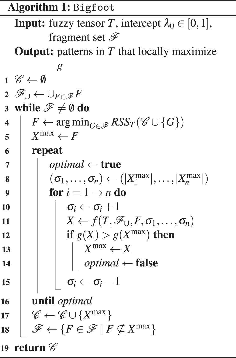
Constraints (7) and (8) force all variables wt and xe to be either 0 or 1. wt=1 if the n-tuple t is in the returned pattern. xe=1 indicates that at least one of those n-tuples, with wt=1, involves the element e. f therefore returns X=i=1n{eDi|xe=1}. As detailed later, Constraint (4) forces the values of all variables wt and xe to be coherent with the syntactic definition of a pattern (see Section 2). Constraint (5) forces the returned pattern X to be a super-pattern of the grown fragment F, i. e., XF. Finally, Constraint (6) forces X=i=1nXi to satisfy i{1,,n}, |Xi|=σi. Given those constant cardinalities, |X| is constant too. It is i=1nσi. That is why maximizing g(X)=|X|λX2=tXTtλ02|X| amounts to maximizing tX(Ttλ0).

However, according to Problem (3), f maximizes a slightly different sum: twt(Ttλ0). Given 's definition, at line 2 of Algorithm 1, the terms that relate to n-tuples that are not in any fragment are missing. f therefore assumes t, Tt=λ0. In other terms, f maximizes g in an approximation T̃ of the tensor T: T̃t=Tt if tλ0 otherwise. If the fragments include all the n-tuples in the patterns composing the desired model X, i. e., if XXX, then the approximation is harmless. However, the fragments do not need to include all these n-tuples. Indeed, f returns i=1n{eDi|xe=1} (and not {t|wt=1}), which can include n-tuples absent from .

The reason why f assumes t, Tt=λ0 is simple: for a fast resolution of the ILP problem, its number of variables ought to be small. Thanks to the assumption, Constraints (7) and (8) “only” define || variables wt and i=1n|{ti|t}| variables xe rather than, respectively, i=1n|Di| and i=1n|Di| without the assumption. A smaller number of xe variables is particularly interesting because the ILP solver only branches on the xe variables. Indeed, a valuation of the xe variables implies a unique valuation of the (more numerous) wt variables, according to Constraint (4), which equates to

t,wt=1i{1,,n},xti=1.

Finally, at line 11 of Algorithm 1, giving g(Xmax) as an additional argument to the function f allows to add the following constraint for a faster resolution of every ILP problem, without any alteration of Algorithm 1's output:

tTwt(Ttλ0)>g(Xmax)i=1nσi.(9)

i=1nσi is the area of the pattern X that f must return. Under the assumption t, Tt=λ0, Constraint (9) equates to g(X)>g(Xmax). Since f's output only matters if the test at line 12 of Algorithm 1 passes, Constraint (9) safely prunes the search space.

4.2. Bigfoot-LR

f, called at line 11 of Algorithm 1, may take exponential time to solve the ILP problem. For a polynomial time complexity, f can, instead, solve the linear relaxation of the problem, where Constraint (7) is substituted by

t,wt[0,1].

To maximize twt(Ttλ0) (Problem (3)), wt must be maximal for all t. However, Constraint (4) (the only constraint involving the wt variables) forces 0i=1nxtinwt. As a consequence, every wt must be valuated to i=1nxtin and the linearly relaxed problem is the maximization of

ti=1nxtin(Ttλ0)=1ni=1ntxti(Ttλ0)
under Constraints (5), (6) and (8).

Taking the n-tuples in slice by slice (definition in Section 2), the problem becomes the maximization of

1ni=1neDixet s.t. ti=e(Ttλ0)(10)
under Constraints (5), (6) and (8).

Given the inputs of Algorithm 1, the innermost sums (one sum for each element ei=1nDi) are constants. They only need to be computed once, before running Algorithm 1. A greedy algorithm solves the problem in an exact way. First of all, Constraint (5) forces xe=1 for all elements e involved in the fragment F. Then, additional xe variables are set to 1 to satisfy Constraint (6): those with e in the proper dimension and the greatest t s.t. ti=e(Ttλ0). Lines 2 and 3 in Algorithm 2 respectively select those two types of elements.

Bigfoot-LR is the name given to Algorithm 1 when f solves Problem (10) with Algorithm 2. Algorithm 2 is fast. It runs in O(i=1nσi) time. However, only growing the fragments with n-tuples in the densest slices of is naive. Section 5 shows that Bigfoot-LR returns patterns that are only slightly larger than the fragments.

Nevertheless, Bigfoot can further grow those patterns. They become the argument of a second execution of Algorithm 1, this time without the linear relaxation of the ILP problem. Being larger than the initial fragments, Bigfoot-LR's patterns save some iterations of Bigfoot's hill-climbing. On the other hand, altogether, Bigfoot-LR's patterns include more n-tuples than the initial fragments and solving the individual ILP problems takes more time. TriclusterBox, discussed in Section 3.2, is less naive than Bigfoot-LR. However, it cannot provide “larger fragments” to Bigfoot. Indeed, Bigfoot would not grow them because they already locally maximize g.

4.3. Forward Selection

The disjunctive box cluster model composed of all the patterns that Bigfoot, Bigfoot-LR or Bigfoot-LR+Bigfoot outputs overfits the fuzzy tensor. A well-chosen subset of those patterns usually makes a statistically more relevant model, i.e., a simpler (with fewer patterns) disjunctive box cluster model (1) whose residual sum of squares (2) is not significantly higher. Stepwise regression aims to heuristically select such a subset of the candidate explanatory variables (the computed patterns). The search of a trade-off between the goodness of fit and the simplicity is formalized as the minimization of a measure, e.g., the Akaike information criterion (AIC) [3]. Assuming that, for any subset X of the set C of computed patterns, the residuals TtT̂t follow an independent identical normal distribution with zero mean, AICT(X) is

2|X|+|CCC|ln(RSS{tTt|tCCC}(X)).

That formula considers that the models, the subsets of C, only predict the membership degrees of the n-tuples in CCC. It disregards every n-tuple tCCC because XC, T̂t=λ0. Besides, unless λ0 is the average membership degree over these n-tuples, the mean of the residuals would not be zero, a violation of one of the assumptions behind the formula. Those same arguments stand when it comes to assessing the quality of the selected model XC, i.e., AICT should disregard every n-tuple tXXX. That is why the proposed stepwise regression is recursive: it first selects a subset X1 of C, then a subset X2 of X1 (substituting C by X1 in the formula above), etc. That process stops at iteration k if Xk=Xk1 (a fixed point) and Xk is the disjunctive box cluster model that is returned.

Algorithm 3 formalizes the recursive forward selection (the chosen stepwise regression technique) of the disjunctive box cluster model XC. At every iteration, line 3 takes from C the pattern that, added to X, minimizes RSST (and AICT), i.e., that best complements the current model. That selection is analogous to that of line 4 in Algorithm 1. As explained in Section 4.1, it takes O(CC|C|)-time and favors the selection of a pattern not intersecting much the previously selected patterns, because the predicted membership degrees for the n-tuples in the intersection can only marginally increase. If adding to X any more pattern, taken in C, would increase AICT (line 4), the selected patterns become the candidate patterns of a new forward selection (line 5). The recursion terminates when all candidate patterns are selected (line 2). Line 7 returns them.

5. EXPERIMENTAL VALIDATION

multidupehack [11], Bigfoot, Bigfoot-LR and TriclusterBox [2] are all distributed under the terms of the GNU GPLv3. They are implemented in C++ and compiled by GCC 5.4.1 with the O2 optimizations. The implementation in C of Walk'n'Merge[16] was provided by its authors. DBTF [20] is only distributed in binary form. All experiments are performed on a GNU/LinuxTM system. It runs on top of 2.4 GHz cores, 12 MB of cache and 32 GB of RAM. Bigfoot uses IBM ILOG CPLEX Optimizer [22] v12.6.0 to solve the ILP problems. https://gitlab.com/lucasmaciel82/Bigfoot hosts the datasets, the source codes (including for the generation of synthetic tensors) and the scripts to run all the experiments.

5.1. Real-world Tensors

5.1.1. A 3-way tensor

The first real-world fuzzy tensor used in this section is 3-way. It indicates how influential the messages that a Twitter user (among 170,670) wrote about a Brazilian soccer team (among 29, identified by supervised classification) during a week (among 12 in 2014, from January 13th to April 6th). The influence (i.e., the membership degree) is here defined from how many times the messages were “retweeted” and from the overall popularity of the team: the numbers of retweets for a given team are multiplied by a constant chosen so that the sum of the normalized numbers is the average number of retweets per team; a logistic function, with a growth rate of 0.5 and centered on 10 normalized retweets (as shown in Figure 1), turns each normalized number of retweets into an influence, in [0,1]. Summing all influences gives 40,167.3, i.e., 40,167.3170,670×29×120.0006 times the maximal possible value. Because λ0=0.0006 minimizes RSST(), it can be considered the default setting. Here, λ0 is set to 0.1, to discover more and denser (although smaller) patterns.

Figure 1

Curve of the logistic function chosen to turn normalized numbers of retweets into influence degrees: 10 normalized retweets map to “moderately influential.”

multidupehack [11] provides the fragments. Three minimal size constraints are enforced (see Section 3.1): at least eight users, three teams and four weeks. With the upper-bounds ϵuser=3, ϵteam=8 and ϵweek=6 (again, see Section 3.1), there are 1,183,653 fragments. multidupehack returns them within 47.4 seconds. Given their minimal sizes and the upper-bounds, any slice of any fragment has, at least, a 0.75 density. Bigfoot-LR takes 2 minutes and 20 seconds to turn the 1,183,653 fragments into only 44 distinct patterns. The high degree of overlap between multidupehack's patterns and Bigfoot-LR's addition of elements by decreasing order of density together explain why that number is so small: many fragments grow into a same pattern. Bigfoot processes Bigfoot-LR's 44 patterns within 52 seconds and the forward selection only keeps two patterns. The first pattern is large and rather dense: λX+λ0=0.81. It involves all 12 weeks, 110 influential supporters and journalists and 13 famous teams (most of them from the Southeast region of Brazil), hence 17,160 3-tuples. The second pattern is smaller, 150 3-tuples, but denser, λX+λ0=0.85. It only involves teams and supporters from the South region of Brazil. Bigfoot alone takes more than ten hours (at which point it was aborted) to process the 1,183,653 fragments.

However, Bigfoot can directly process, in a reasonable time, an alternative collection of fragments. By reducing the minimal number of teams in a fragment to two but forcing these fragments to be denser (with ϵuser=0.5, ϵteam=2 and ϵweek=1, i.e., a minimal possible density of 0.875), multidupehack takes 1.1 second to provide 359 fragments. Within 6 hours and 54 minutes, Bigfoot and the forward selection turn those fragments into six patterns. The first three columns of Table 3 list them in the order Algorithm 3 selects them, i.e., from the pattern that most reduces RSST to the one that least contributes to the model. Their first two dimensions are large. That is why Table 3 only reports their cardinalities.

|Xuser| |Xweeks| Xteams λX+λ0
{Botafogo, Flamengo,
31 12 Fluminense, Vasco} 0.702
28 11 {Corinthians, Palmeiras, Santos} 0.754
14 10 {Avaí, Figueirense} 0.864
17 7 {Grêmio, Internacional} 0.859
15 11 {Flamengo, Fluminense} 0.792
17 12 {Flamengo, Vasco} 0.801
Table 3

Disjunctive box cluster model, discovered by Bigfoot, of the 170,670×12×29 retweet tensor.

Every discovered pattern only involves teams from one single state. For example, the first pattern involves four teams from Rio de Janeiro. The explanation is simple: who is influential when writing about a given team is likely influential when writing about its rivals, in the same state. The identifiable users involved in a given pattern are either journalists, who are indeed influential, or supporters of one of the teams in the pattern. The first four patterns do not intersect, a property favored by the forward selection, as explained in the last paragraph of Section 4.3. The last two patterns intersect with each other and with the first pattern in the table. Yet, their addition to the disjunctive box cluster model makes it significantly more accurate (smaller AICT). The last column of Table 3 gives the densities of the patterns. The patterns are large and dense. Within 2.7 seconds, Bigfoot-LR grows the same 359 fragments into 46 slightly larger fragments.

TriclusterBox [2], Walk'n'Merge [16] and DBTF [20] only handle 0/1 tensors. To use them, every membership degree in the fuzzy tensor is rounded to 0 or 1. It takes TriclusterBox ten hours of computation to only grow one single pattern out of 12×29=348 (see Section 3.2). Despite many attempts with different minimal size and density parameters, Walk'n'Merge only outputs two patterns within 2 hours and 19 minutes (average run time over the attempts): one very large and sparse pattern involving all weeks, 597 users and 24 teams, and one very dense pattern of size 2×2×2. DBTF's configuration includes the number of patterns to discover. However, even if that parameter is set to 30, DBTF does not discover any pattern: it either crashes or one of the returned factors is null.

5.1.2. A 4-way tensor

The second real-world application analyzes the usage of the bicycle sharing network in Lyon, France. That network consists of 327 stations where bicycles can be rented and returned. The riding behaviors evolve along the day and depend on the day of the week. That is why 7×24 directed graphs (one per day of the week and per one-hour period) are built from a two-year log of the system. Their edges are labeled with the numbers of rides between every ordered pair of stations. Those numbers are normalized so that every directed graph has a same total weight. Finally, a logistic function turns every normalized number of rides into a membership degree. The resulting 7×24×327×327 fuzzy tensor has a 0.005 density. λ0 is set to that value.

To discover in the 7×24 graphs some kind of cross-graph quasi-cliques, i.e., days of the week and periods of these days, during which many users ride between stations in one single set, the departure and arrival stations in a pattern must be constrained to be the same. multidupehack can do so [11]. To have Bigfoot explore that same restricted pattern space, one additional constraint is added to the ILP problem that f solves at line 11 of Algorithm 1:

t,xtdeparture=xtarrival.

The hill-climbing procedure has to be modified too: at line 9 of Algorithm 1, one single index stands for both the departure and the arrival stations and the related iterations increment/decrement both σdeparture and σarrival at lines 10 and 15. Those simple changes, which demonstrate the adaptability of the proposal, reduce the time requirements because more constrained ILP problems are easier and because hill-climbing in a smaller pattern space is faster.

With ϵdeparture=ϵarrival=21.6, ϵhour=14.4 and ϵday=28.8, multidupehack takes 2 minutes and 44 seconds to return 5,462 fragments with at least four stations, six one-hour periods and three days (hence a minimal possible density of 0.7). Bigfoot grows them within 5 hours and 40 minutes. Algorithm 3 then selects two patterns. Figures 2 and 3 show the geographic positions of the stations involved in those patterns. Their captions report the associated days of the week and periods of the day. The available implementations of TriclusterBox, Walk'n'Merge and DBTF are restricted to mining 3-way 0/1 tensors: they cannot be used here.

Figure 2

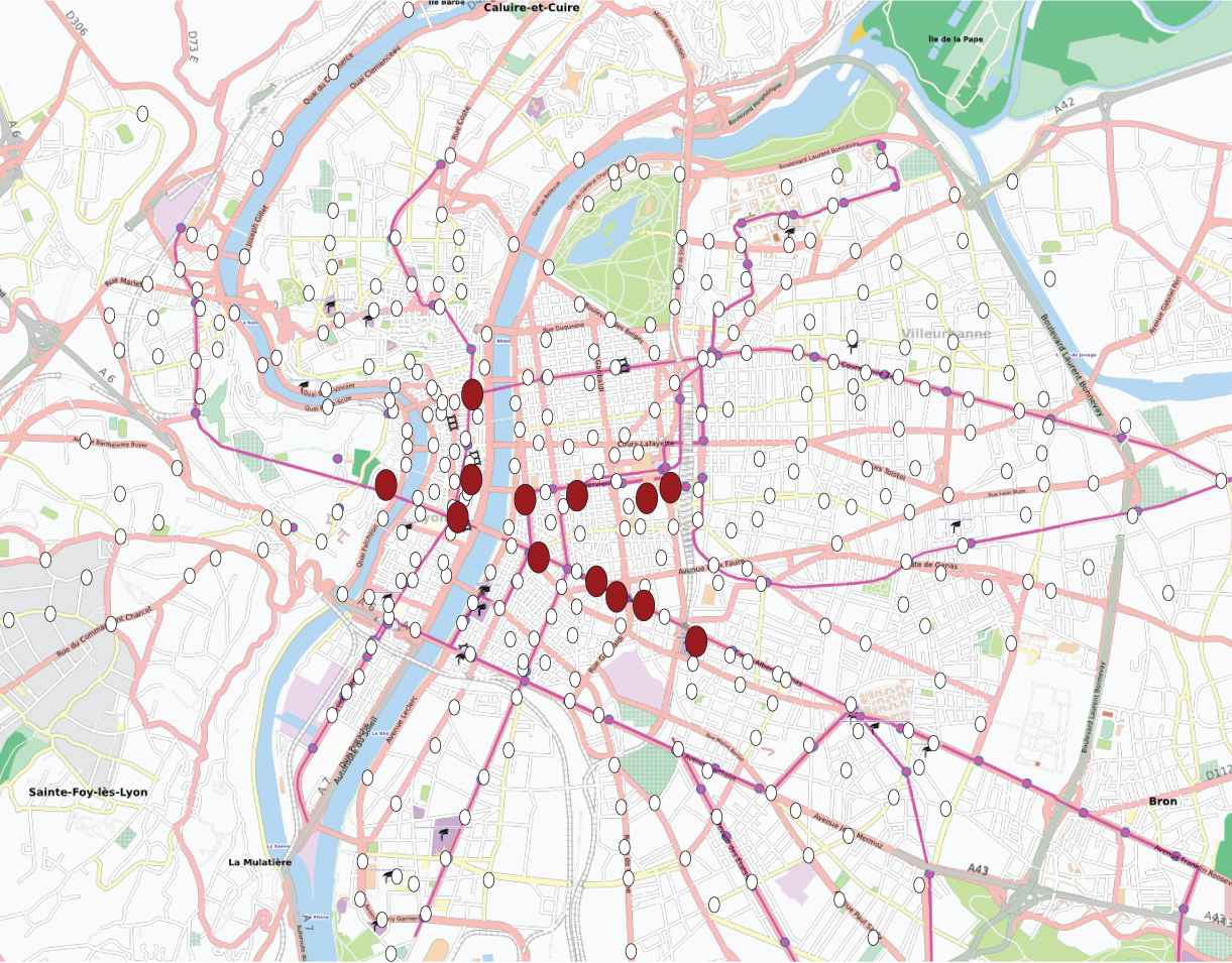
Thirteen large stations in the working and commercial districts of Lyon. They exchange many bicycles everyday from midday to 8pm, except on Sundays, when the shops are closed. |X|=8.112 and λX+λ0=0.383.

Figure 3

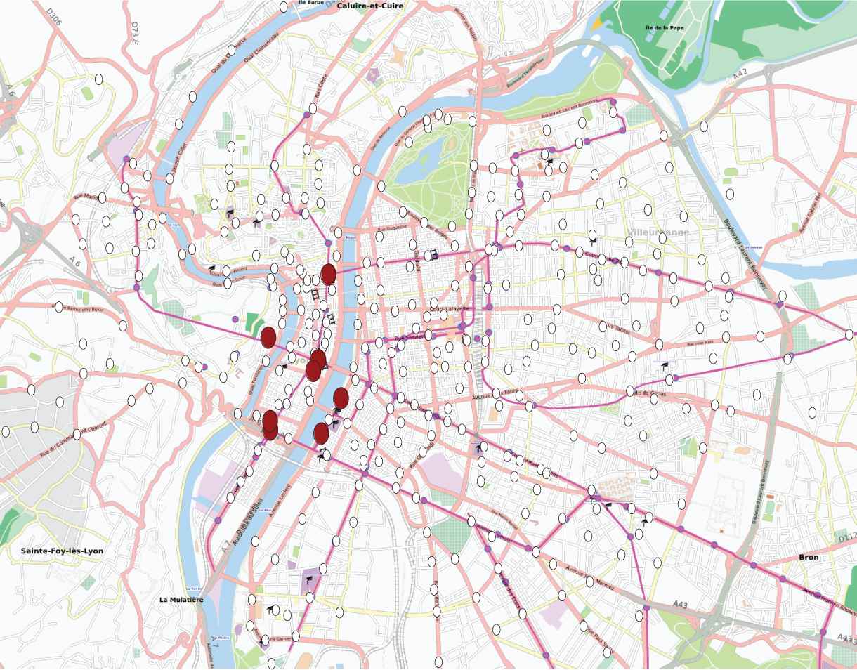
Eight large stations around the main squares of Lyon, in its historical center. Everyday, from 8am to 10am and from midday to 9pm, many users ride between those stations. |X|=4,928andλX+λ0=0.256.

5.2. Synthetic Tensors

The actual patterns to discover in real-world tensors are unknown. To assess to what extent Bigfoot and its variations can recover patterns, this section uses synthetic tensors affected by controlled levels of noise. Four “perfect” patterns (i.e., only containing 3-tuples with membership degrees equal to 1) of sizes 6×6×6 are randomly planted in a null 32×32×32 tensor. With those settings, the patterns often overlap, what happens in real-world contexts too, e.g., in Table 3 or in Figures 2 and 3.

Considering every 0 or 1 in a “perfect tensor” as the output of a Bernoulli variable with parameter p, the probability of a 1, inverse transform sampling allows to noise the tensor. The posterior distribution of p is the beta distribution of parameters α and β, which have a meaningful interpretation: after observing, for a same n-tuple, α1 membership degrees at 1 and β1 at 0, the beta distribution is the distribution of p. Choosing a number of correct observations (α1 when noising a 0, β1 when noising a 1) and a number of incorrect observations (β1 when noising a 0, α1 when noising a 1) therefore defines the level of noise applied by inverse transform sampling. In these experiments, the number of incorrect observations is always set to 0, i.e., only the number of correct observations tunes the level of noise. More correct observations lead to membership degrees that are closer to the values in the “perfect” tensor. Figure 4 plots the inverses of cumulative beta distributions that are used to noise a 0 in a “perfect” tensor: a uniformly random abscissa is drawn in [0,1] and the related ordinate is read on the curve whose number of correct observation provides the desired level of noise. That ordinate is the noisy version of the 0 in the “perfect” tensor.

Figure 4

Inverses of cumulative beta distributions used to noise a membership degree at 0 in a “perfect” tensor. More “correct observations” mean less noise.

Given a planted pattern P and a pattern X at the output of a method, the Jaccard index |PX||PX| measures their similarity. Given P, the planted patterns, and X, the patterns discovered in the related fuzzy tensor, the quality of X is here defined as

PPPargmaxXX|PX||PX|PPPXXX.

That measure, in [0,1], is a ratio between numbers of n-tuples. At the numerator, the true positive n-tuples are both in a planted pattern and in the pattern of X that is the most similar. The denominator is the number of n-tuples in the planted patterns or in the discovered patterns. The quality measure penalizes both the absence from X of patterns that are similar to the planted ones and the discovery of patterns including n-tuples out of the planted patterns. It does not penalize the discovery of supernumerary overlapping patterns. That is why the following experimental results report as well the number of patterns that are discovered, |X|.

Figure 5 shows the quality of the discovered patterns, their numbers, and the run times, in function of the level of noise in the 3-way fuzzy tensor. In this section, λ0 is always set to 0. For a given level of noise, all results are averages over eight randomly generated tensors. multidupehack [11] provides the fragments, with at least three elements of every dimension. Different upper-bounds (ϵ1,ϵ2,ϵ3) are tested so that the fragments can be more or less dense. The upper-bound is always the same whatever the dimension, i.e., ϵ1=ϵ2=ϵ3=ϵ. It relates to μ, whose values are written above the plots: ϵ=32(1μ). For instance, for μ=0.6 (rightmost plots), multidupehack's upper-bounds are (3.6,3.6,3.6). Given multidupehack's definition of a fragment and the minimal size constraints, μ=1ϵ32 is the minimal possible density for any slice of a fragment. Forward selection (see Section 4.3) is used to simplify the output of all methods but multidupehack's, so that the overall gains can be observed. Whatever the method, the forward selection improves the quality and, of course, decreases the number of patterns. The reported run times include that step.

Figure 5

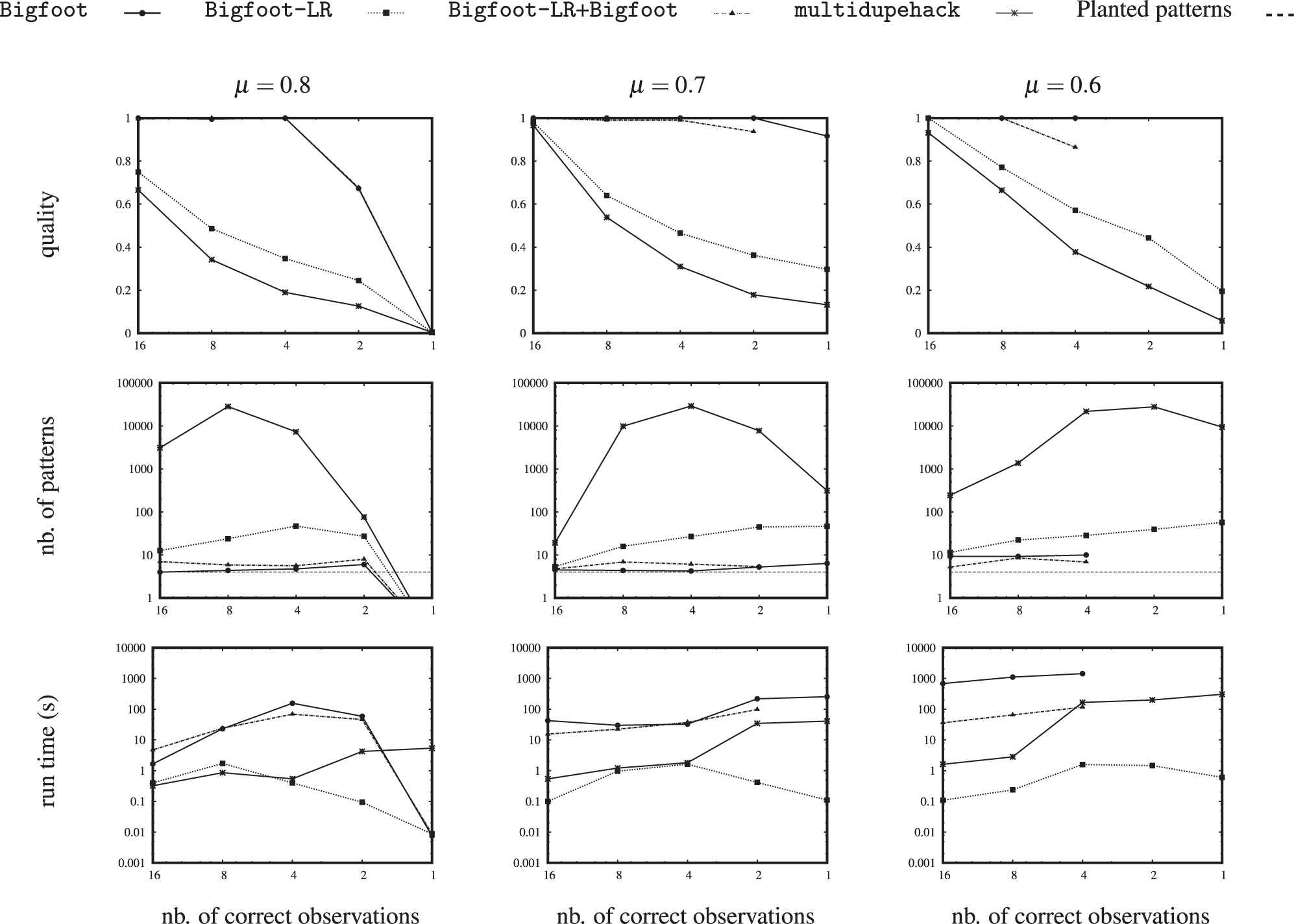
Qualities, numbers of patterns and run times of multidupehack, Bigfoot, Bigfoot-LR and Bigfoot-LR+Bigfoot mining noisy 3-way tensors (the level of noise increases from left to right).

Figure 6

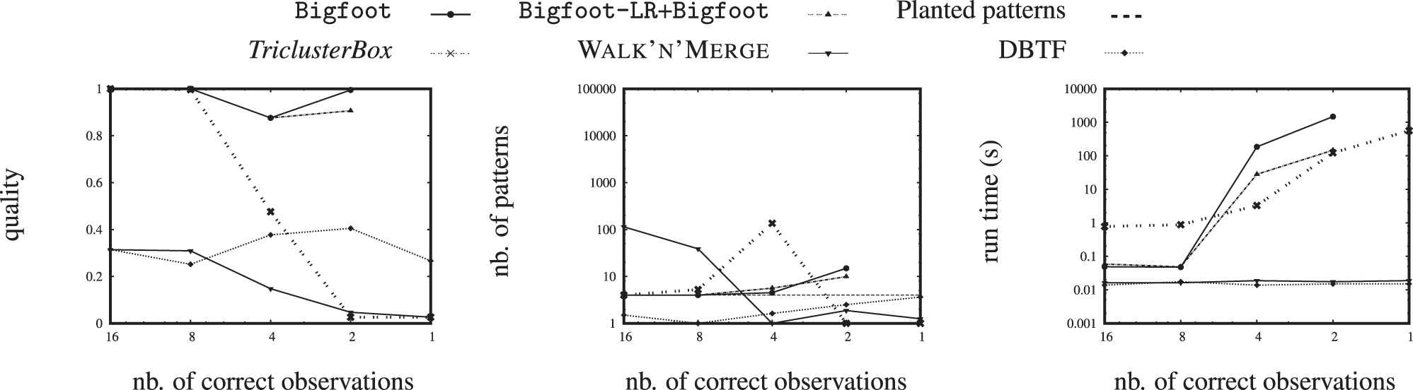
Qualities, numbers of patterns and run times of the competing methods mining noisy 3-way 0/1 tensors (the level of noise increases from left to right).

multidupehack returns up to hundreds of thousands of fragments. They poorly match the planted patterns, unless the level of noise is very low (16 correct observations). Nevertheless, Bigfoot and Bigfoot-LR+Bigfoot, which both process multidupehack's outputs, reach significantly higher qualities after the forward selection that keeps numbers of patterns that are close to four, the number of planted patterns. Bigfoot is always the best performer. That is, when it is actually given fragments to grow and when it runs within one hour, the chosen timeout. Bigfoot can indeed require much time, especially to grow fragments of low density in noisy tensors. Bigfoot-LR is very fast but it returns terrible patterns, enhanced fragments that need more growing. Using Bigfoot to further grow them, Bigfoot-LR+Bigfoot often outputs the same patterns as Bigfoot alone. When it does not, the obtained qualities are slightly lower. Given the least dense fragments (μ=0.6), Bigfoot-LR+Bigfoot does not even take one tenth of the time Bigfoot requires. However, it may be slower, e.g., to grow the fragments with μ=0.7 in the noisiest tensors. The end of Section 4.2 explains why. In presence of little noise (at least 4 correct observations), Bigfoot always recovers the four planted patterns, whatever the tested minimal density μ of the provided fragments. With μ=0.8, multidupehack returns too few fragments in the noisier tensors to recover the planted patterns, whereas μ=0.7 allows Bigfoot's patterns to exceed the 0.9 quality, even in the noisiest setting (1 correct observation).

Bigfoot and its variations handle n-way fuzzy tensors. In contrast, the state of the art only deals with 3-way 0/1 tensors. After rounding to 0 or 1 the membership degrees of the same noisy tensors used above, Bigfoot and Bigfoot-LR+Bigfoot can be compared to TriclusterBox, Walk' n'Merge and DBTF. The minimal density parameter of Walk'n' Merge's is set to 0.7; its other parameters to their default values. Walk'n'Merge uses the Minimal Description Principle to not overfit the tensor. TriclusterBox includes no such mechanism and the forward selection, described in Section 4.3, always improves its output. TriclusterBox's results in Figure 6 include that step. The number of patterns DBTF should discover is part of its configuration. Although that number is set to the number of planted patterns, four, DBTF sometimes returns fewer patterns. multidupehack still provides the fragments that Bigfoot and Bigfoot-LR+Bigfoot grow. It is configured as earlier and μ is set to 0.7. Here, that means any slice of any fragment contains at most two 3-tuples with null membership degrees.

Figure 6 shows that Bigfoot does not always reach the qualities reported in Figure 5: rounding to 0/1 harms the ability to recover the planted patterns. Despite that, Bigfoot and, to a lesser extent, Bigfoot-LR+Bigfoot, are clearly better than TriclusterBox, Walk'n'Merge and DBTF at recovering the planted patterns from the noisy 0/1 tensors. The competitors are faster though, especially in the noisiest settings.

6. CONCLUSION

Discovering a disjunctive box cluster model is a problem that generalizes the Boolean CP tensor factorization: every pattern (rank-1 tensor) is weighted by a parameter to estimate. Searching for patterns one by one, the optimal weights simply are their densities. Such a disjunctive box cluster model therefore is more informative than a Boolean CP factorization but it remains easy to interpret. Moreover, it suits fuzzy tensors and not only 0/1 tensors.

This article has presented the first solution to decompose fuzzy tensors into patterns. It grows pattern fragments and selects a small number of grown patterns to fit but not overfit the fuzzy tensor. Various techniques have been combined. In particular, every pattern is grown by hill-climbing and an integer linear model has been defined to have an existing solver efficiently find the pattern at the next iteration. Since solving ILP problems may take exponential time, a linearly relaxed variation of the problem has been presented as well. The related algorithm is less effective but can be used in a preprocessing step. Finally, a recursive forward selection composes the returned model, a subset of the grown patterns, by greedily minimizing the AIC.

Experiments have shown that the method successfully recovers patterns in noisy synthetic tensors. It even outperforms state-of-the-art approaches when the tensor is 0/1, a special case. Relevant patterns have been found in two real-world fuzzy tensors with tens of millions of values. Future work includes extending the integer linear model and exploring other algorithmic approaches to even more accurately and efficiently fit a disjunctive box cluster model to a fuzzy tensor.

CONFLICTS OF INTEREST

The authors have no conflict of interest to declare.

AUTHORS' CONTRIBUTIONS

Lucas Maciel designed, implemented and evaluated most of the proposal. Jônatas Alves helped him with the experiments on synthetic tensors; Vinicius Fernandes dos Santos with the definition of the ILP problem; Loïc Cerf with the forward selection, the computation of argminCCRSST(XC) and the generation of synthetic tensors. Together, Lucas Maciel and Loïc Cerf did most of the literature survey and most of the writing.

ACKNOWLEDGMENTS

The work has been partially funded by the Fundação de Amparo à Pesquisa do Estado de Minas Gerais under Grant number APQ-04224-16.

APPENDIX

This appendix deals with the efficient computation of argminCCRSST(X{C}), at line 4 of Algorithm 1 and at line 3 of Algorithm 3. Section 4.1 has already shown its time complexity is O(CC|C|), because, at a given iteration of Algorithm 1 or 3, RSST(X) is a constant and the difference RSST(X{C})RSST(X) only depends on the membership degrees and the predicted membership degrees of the n-tuples in CC.

However, the worst patterns in C need not even be considered if information computed in previous iterations of those algorithms is kept in memory. The idea is to store along every pattern CC, a lower bound of RSST(X{C})RSST(X), where X is any model that can be obtained at any future iteration. In this way, at any future iteration, if the lower bound associated with a pattern CC exceeds the smallest difference of RSST found so far, C cannot be the pattern to select. Given (1) and (2), if T̂t is the membership degree that the future model X predicts for the n-tuple tC, RSST(X{C})RSST(X) is

tC(max(T̂t,λ0+λC)Tt)2(T̂tTt)2.

A lower bound of that sum is the sum of its negative terms. The term relating to the n-tuple tC is negative if and only if

|max(T̂t,λ0+λC)Tt|<|T̂tTt|T̂t<λ0+λC<2TtT̂t.

The smaller T̂t is, the weaker the condition and the greater the number of negative terms. Moreover, a minimal T̂t minimizes the negative term, (λ0+λCTt)2(T̂tTt)2. Indeed, a consequence of the inequality above is T̂t<Tt. Algorithms 1 and 3 never remove patterns that were previously added to the model. That is why X is necessarily a superset of the model at the current iteration and, given (1), tC, T̂tT̂t, where T̂t is the membership degree that the current model predicts for the n-tuple t. A lower bound of RSST(X{C})RSST(X) at the current iteration therefore is

tC s.t. T̂t<λ0+λC<2TtT̂t(λ0+λCTt)2(T̂tTt)2.

That lower bound is tight. It is reached when future iterations add to the model patterns at least as dense as C that altogether include every n-tuple tC such that λC>2TtT̂t and no pattern that modifies the prediction T̂t of the membership degree of any tC such that T̂t<λ0+λC<2TtT̂t.

The patterns in C are stored in a self-balancing binary search tree that is ordered by increasing lower bound. The initial lower bounds—tC s.t. 0<λC<2(Ttλ0)(λ0+λCTt)2(λ0Tt)2, for all CC —are computed before the first iteration of Algorithm 1 or 3. Algorithm 4 (below) computes argminCCRSST(X{C}). Every iteration starts by taking the first pattern C out of C (line 3). Lines 4–9 compute RSST(X{C})RSST(X) and the lower bound associated with C, given the current model X. Iterations stop (line 2) when C is empty or, more commonly, when its first pattern is associated with a lower bound that is larger than the smallest difference of RSST found so far (lines 11–12). Lines 13–14 reinsert in C the patterns that were taken out of it and whose lower bounds were updated, except the returned pattern.

Footnotes

1

Bigfoot stands for Bigfoot Is Growing Fragments Out Of Tensors. It did not exist in nature. We designed it.

REFERENCES

22.E. Robert, Bixby, ILOG, and IBM, CPLEX Optimizer, 1988. https://www.ibm.com/analytics/cplex-optimizer/
Journal
International Journal of Computational Intelligence Systems
Volume-Issue
13 - 1
Pages
1036 - 1047
Publication Date
2020/07/29
ISSN (Online)
1875-6883
ISSN (Print)
1875-6891
DOI
10.2991/ijcis.d.200715.002How to use a DOI?
Copyright
© 2020 The Authors. Published by Atlantis Press B.V.
Open Access
This is an open access article distributed under the CC BY-NC 4.0 license (http://creativecommons.org/licenses/by-nc/4.0/).

Cite this article

TY  - JOUR
AU  - Lucas Maciel
AU  - Jônatas Alves
AU  - Vinicius Fernandes dos Santos
AU  - Loïc Cerf
PY  - 2020
DA  - 2020/07/29
TI  - Climbing the Hill with ILP to Grow Patterns in Fuzzy Tensors
JO  - International Journal of Computational Intelligence Systems
SP  - 1036
EP  - 1047
VL  - 13
IS  - 1
SN  - 1875-6883
UR  - https://doi.org/10.2991/ijcis.d.200715.002
DO  - 10.2991/ijcis.d.200715.002
ID  - Maciel2020
ER  -