
Novel Optimization Based Hybrid Self-Organizing Map Classifiers for Iris Image Recognition
 , D. Jude Hemanth1, *
- DOI
- 10.2991/ijcis.d.200721.001How to use a DOI?
- Keywords
- Biometrics; Artificial neural network; Hybrid classifier; Optimization; Iris
- Abstract
The concern over security in all fields has intensified over the years. The prefatory phase of providing security begins with authentication to provide access. In many scenarios, this authentication is provided by biometric systems. Moreover, the threat of pandemic has made the people to think of hygienic systems which are noninvasive. Iris image recognition is one such noninvasive biometric system that can provide automated authentication. Self-organizing map is an artificial neural network which helps in iris image recognition. This network has the ability to learn the input features and perform classification. However, from the literature it is observed that the performance of this classifier has scope for refinement to yield better classification. In this paper, heterogeneous methods are adapted to improve the performance of the classifier for iris image recognition. The heterogeneous methods involve the application of Gravity Search Optimization, Teacher Learning Based Optimization, Whale Optimization and Gray Wolf Optimization in the training process of the self-organizing map classifier. This method was tested on iris images from IIT-Delhi database. The results of the experiment show that the proposed method performs better.
- Copyright
- © 2020 The Authors. Published by Atlantis Press B.V.
- Open Access
- This is an open access article distributed under the CC BY-NC 4.0 license (http://creativecommons.org/licenses/by-nc/4.0/).
1. INTRODUCTION
The advancement of digital technologies and need for security systems had led to the development of automated recognition system which provides authentication. Such automated systems are used in applications such as border surveillance, national identity, access to private areas, security to personal gadgets and attendance monitoring systems of large firms. Usually biometrics are used as the key factor to build such recognition systems. The biometric traits represent the exceptional attributes of a person. These traits are largely classified as physiological traits and behavioral traits. The physiological traits are derived from the corporeal measurements of human anatomy. Biometric traits like face, fingerprint, hand geometry, iris and DNA are examples of physiological traits. The behavioral traits are derived from detectable attributes of human behavior. Biometric traits like voice, gait, keystroke and signature are examples of behavioral traits. Special acquisition units are used to capture these traits and administer to the automated systems for further processing. The systems are ingeniously modelled to learn the traits and perform recognition involuntarily.
The unique features present in the iris makes it a suitable biometric trait for noninvasive automated recognition systems. It is a thin pigmented diaphragm present in the anterior region of the eye. It controls the quantum of light reaching the retina by regulating the diameter and the size of the pupil. German scientist F.H. Adler [1] and British ophthalmologist J.H. Doggart [2] suggested that photograph of iris can replace fingerprints. This concept was later patented in 1980's by two American ophthalmologists, L. Flom and A. Safir [3] although they did not have enough algorithm to implement it as a human identifier. The iris is multi-layered structure with collagenous fibers and tightly packed heavily pigmented epithelial cells. This intervened network makes the iris region to appear with furrows, freckles, crypts, coronas, rifts, serpentine capillaries and striations. Thus, when captured using optical device, it shows its richness in texture. It is also highly unique such that even a monozygotic twin will have different iris pattern. Moreover, the iris is well protected and properly lubricated, placed safe. In addition, the size and shape remain almost unchanged throughout the life span of the person.
To elucidate on the details of the related works and the results of proposed method the following sections are sub-divided as follows: Section 2 briefs about biometrics. Section 3 presents a detailed look into the related works in literature. Section 4 elucidates the system model. Section 4 illustrates the network model. Section 5 reports the training procedure involved in the hybrid classifier model. Section 6 justifies the results taken the experiments and Section 7 finally draws conclusion.
2. BIOMETRICS
Biometrics are the statistical study of living being to identify them. The improvements in the computational intelligence and VLSI technologies have made faster, easier and secured use of these biometrics to give immediate access to confidential documents or areas through digital authentication. With the integration of biometric technology with different facets, it has the potential to be used in many application. It is found in applications like secured online payments, national ID, law enforcement, gadget security and border control. Several modalities have been in practice to capture these biometric identifiers. Identifiers related to morphology like hand geometry, ears, palmprint, palm veins, fingerprint and iris belong to physiological characteristics and identifiers related to behaviors like gait, voice and keyboard stroke belongs to behavioral characteristics. All these characteristics should be universal, unique, invariable, recordable and measurable. The degree to which, these biometric identifiers has these traits, the more comfortable it will be to adapt these technologies. Out of many of these identifiers, iris is found to be highly unique and invariable over a longer span of a human life. As it is safely protected inside the membrane, the disfiguration due to trauma is very less. Hence, methods for iris biometrics is studied in this work.
3. RELATED WORKS
The first algorithm to automate iris recognition was given by J.G. Daugman [4]. In this the phase information of the iris is captured using 2-D Gabor filter and converted into a 256 byte iris code. The author has also shown that these iris codes are highly significant and statistically independent. The author has used hamming distance as a similarity measure to perform classification. The XOR operation can be done rapidly, and hence speeds up the classification process. However, the iris images are captured in a constrained environment without any occlusion, which is impractical. Yang Hu et al. [5], have devised the iris code as an optimization problem. Markov Random Field model is used to explore the spatial relationship among the iris codes and the less reliable bits in the iris codes are removed. This improves the stability of the iris codes and enhances the performance of the classifier. However, the performance of the iris codes in unconstrained environment is left unexplored. In another work by Debanjan sadhya et al. [6], the dynamic clusters are formed of invariant positions to obtain stability between iris codes of intra-class iris images. Further, the error information from the masks are used to eliminate the noise from the extracted bits. Later, hamming distance measures the similarity with the iris codes in the database. It concludes with future scope of extending the recognition toward secure recognition framework and improvement of efficacy over noisy database.
A faster recognition method for iris images captured from mobile phones was suggested by authors [7]. Here, parallel methods are adopted to extract features from the region of interest. Kolmogorov-Smirnov distance is used to fetch the color information, box counting method is used for fetching texture information and clusters are formed by using morphological operations. The distance based classifier is used to combine the results of the three features. However, the recognition rate is not promising to implement a real-time system. Jianxu Chen et al. [8], have made human interpretable feature like crypt to be detected using morphological operations in a hierarchical manner. And later a multi-dimensional matching method is adopted to overcome the errors due to detection failures. Using density based clustering method the closely packed key feature points are grouped into a single point in the article [9]. By this method the average number of key-points to represent the significant areas of the region of interest is reduced. This benefits at the cost of relatively large processing time. In the article [10], the authors have suggested a method to encode the coarse information of the iris using vocabulary tree and fine information using locally-constrained linear coding. These methods are integrated based on their frequency of appearing into a hierarchical visual codebook. This method mitigates spoofing. And the classification of these iris images are done using support vector machines.
In the article [11] authors have used image transformation and machine learning to learn about the features of the iris with an a posteriori probability. A ten-fold cross validation method is used to establish the performance measures of the classifier. Lately many researchers have started exploring deep learning techniques to implement effective iris recognition system. A deep learning approach is recommended by authors in the article [12]. The features of the iris are derived from convolutional neural network. Bayesian inference and supervised discrete hashing is used to reduce the iris template size. The authors have indicated that cross-spectral iris recognition may further improve by adapting data-dependent hashing algorithm. A modified VGG16 convolutional network is proposed by authors in the article [13]. 50% drop out is employed in pooling layers to avoid over-fitting. This has helped in the identification of left and right irises of the same person can also be distinguished with maximum precision. The Japanese tech giant NEC has partnered with US firm Tascent with much focus on iris recognition [14]. This will accelerate the adoption of biometric systems into government and commercial applications. To bridge the gap of power consumption of Graphical Processing Unit (GPUs) and to support energy efficient biometric system, authors in the article [15] have adapted parallelism in executing the recognition operation. A few other machine learning aspects of iris recognition are detailed in articles [16–23].
The classifiers used for iris recognition are broadly categorized as linear classifiers, neighbor-based classifiers, support vector machines, tree-based classifiers, forest-based classifiers and Artificial Neural Networks (ANN). The advantage of ANN is that, it is a nonlinear, nonparametric model which can perform classification for a large dataset with very little knowledge about the dataset. It operates same as the human brain. To illustrate the working of neurons in human brain, a statistical model was introduced by neurophysiologist Warren McCulloh and mathematician Walter Mc Culloh in 1943. Ever since the genesis, several architectures were proposed to mimic the functioning of the human brain. One of the simplest architectures among ANN is the self-organizing map (SOM). It was developed by Teuvo Kohonen, a finish professor in the 1980s. With unsupervised and competitive learning, it maps the high dimensional data into a discretized low dimension. This representation is termed as a feature map.
The accuracy and simple design of the classifier for iris recognition is addressed by (i) modification of SOM to avoid jitters in the learning process and (ii) optimization of update rule to quicken the learning process and to enhance the accuracy of the classifier. The localization is performed using circular Hough transform to segment the circular iris region from the image. Normalization is accomplished by rubber sheet model proposed by Daugman to eliminate the variation of iris size due to exposure to illumination. Statistical features are extracted from the normalized iris region to feed the attributes into the network for learning and testing purposes. The efficacy of the network is tested iris images from IIT-Delhi database. The performance measures are computed to validate the results obtained from the proposed method.
4. SYSTEM MODEL
The flow diagram of the iris recognition systems commonly used in practise is shown is Figure 1. The recognition systems adapts a classifier which identifies the primal elements present in the input and matches it into its respective class. In many modern classifier algorithms machine learning helps in the classification process. ANN is a part of machine learning which can perform classification. These networks are modelled such that it can be trained. It can be programmed to learn itself. The available dataset is segregated as training set and testing set. The images in the training set are used to train the classifier model. The efficacy of the classifier is evaluated by how well it predicts the images in the testing set correctly. The training can happen by supervised learning, unsupervised learning or reinforcement learning. In this paper, unsupervised learning is used.

Schematic flow diagram of the iris recognition system.
The steps involved in the iris recognition process can be summarized as follows:
Step 1: Eye image is either captured from an optical device or downloaded from a recognized iris database.
Step 2: Apply some preprocessing methods to remove the artefacts present in the raw image.
Step 3: Identify the iris region which is the region of interest from the preprocessed eye image.
Step 4: Given a segmented iris image, transform it into a fixed rectangular block.
Step 5: Implement an approach to extract the significant descriptors from the region of interest and form the feature vector.
Step 6: Input the feature vector to the classifier.
Step 7: Select the best ranked output as the recognized class.
4.1. Iris Database
A database is said to have a huge collection of data, which can be extensively used for validation of algorithms proposed by research communities across a large portion of the world. Imaging devices that can operate in the visible spectrum, 380–780 nm or the near-infrared spectrum, 700–900 nm is used to capture the images. Mostly, the iris images captured in near infrared spectrum are stored in gray scale. Successful experimentation of iris recognition algorithms requires iris datasets. To cross validate and compare the performance of the algorithms, researchers need a publically available database to demonstrate the effectiveness of their algorithm. The images collected in the database should represent all the artifacts experienced in real-world environment, images collected from diversified subjects and has to be sufficiently large and publically available.
A Korean company named JIRIS, introduced the first commercially available iris scanner JPC 1000 which can acknowledge the individual based on iris pattern in less than 1 second. Weighing around 80 grams, it can be easily connected to PC via USB. It has software to encrypt and decrypt the data. Thus it provides security for the users. The focal length of it is approximately 15 cm. The details about JIRIS JPC 1000 is available in the following link https://jiristech.en.ecplaza.net/products/jpc1000-iris-recognition-camera-sensor-module-205986. The IIT Delhi iris dataset consists of iris images collected at IIT Delhi. This dataset was acquired using a JIRIS JPC1000 digital CMOS camera, from 224 users and all the images are in bitmap format. The users were between the ages of 14 and 55 years. The 1120 images are from 176 males and 48 females. All images are at a resolution of 320 × 240 pixels.
Figure 2 shows a few samples of iris images collected from IIT-Delhi iris database. Most of the images suffer from low contrast because of nonuniform infrared illumination.
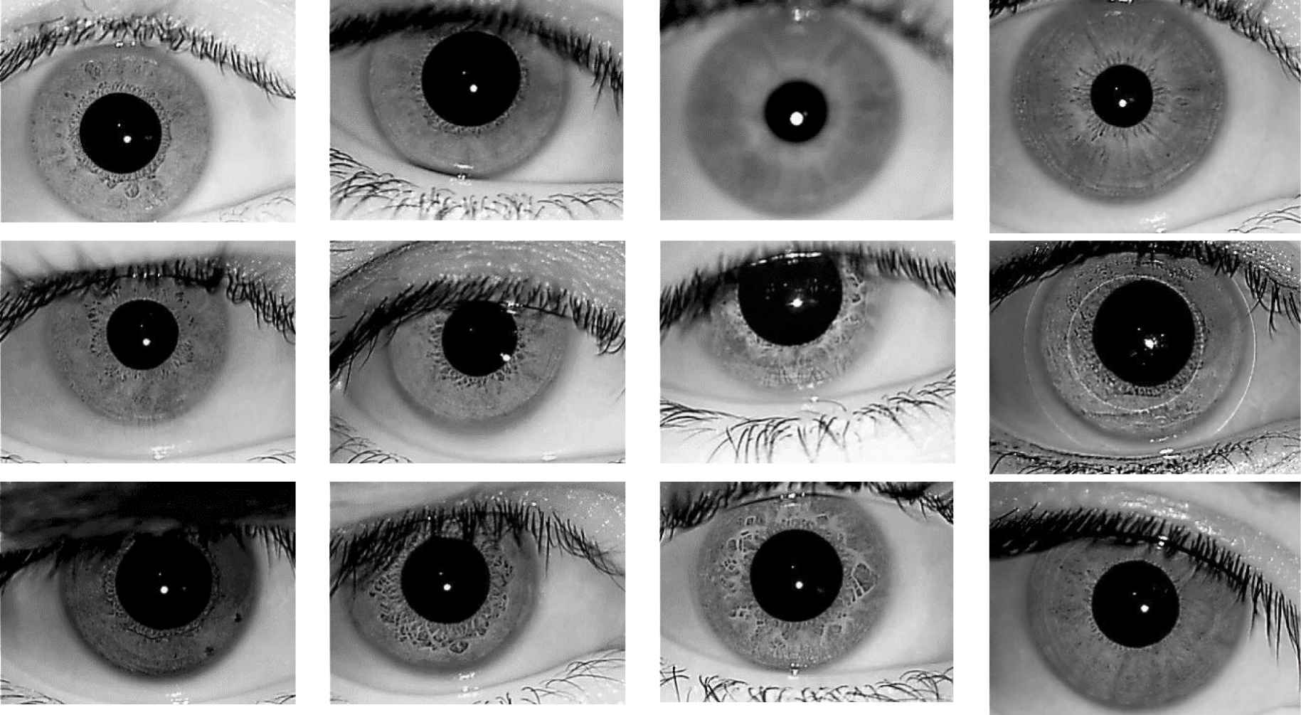
Sample images from IIT-Delhi database.
4.2. Image Enhancement
The iris region is rich in texture. However, if the illumination is not proper, the fine details of the iris may go unnoticed. Moreover, it can affect the segmentation process as well. This errors may ripple through the further stages and affect the performance of the classifier. So, an enhancement method is applied to overcome the illumination variance happened during the acquisition. Here, contrast limited adaptive histogram equalization method is used to enhance the texture region of the eye image.
4.3. Segmentation
The iris is a toroid structure present between the pupil on the inside and the sclera on the outside. The pupil boundary and the sclera boundary locates the iris region. Each boundary is approximately in the shape of a circle. But they are not concentric. The iris localization algorithms employ strategies to identify the center and radius of the two boundaries to segregate the iris region from the image. The iris region holds the actual texture information which is unique. This is used for feature extraction and classification. Hence, the influence of localization on the recognition accuracy is high.
The circular elements present within an image can be discovered by using Circular Hough Transform as described by Hough [24]. Tian et al. [25] have accomplished this for iris recognition. We use this concept to detect the iris in the image, as the pupil boundary and the sclera boundary trace almost a circular geometry. The gradients of the image are computed using an operator like Sobel, Prewit or Laplacian. This gives the edge map of the image. The circle fitting the edge map is found from the maximum accumulated peak point in the parameter space. This procedure helps to identify the iris region separately from the image. It is highly reliable in detecting the object edges from the image and has high accuracy. The boundary of the iris region becomes clear after the localization procedure. This localized iris is used for normalization and feature extraction in the subsequent procedures.
4.4. Normalization
The eye when exposed to illumination, the pupil of the eye elongates or shrinks based on the degree of brightness. This causes the size of the iris region to vary. Hence, collecting features from this iris will not be reliable all the time. To standardize the procedure, the circular iris region is mapped into a rectangular block of fixed size. This eliminates the ambiguity that occurs in the iris size due to illumination. In this work normalization method called rubber sheet model is used. It was proposed by Daugman [4]. In this model, each point in the iris region is plotted into a rectangular block, regardless of the change in pupil dilation and its size. It is also termed as a mapping from Cartesian coordinates
4.5. Feature Extraction
The feature vector is the numerical way of representing an object in machine learning. It is a very crucial process, as the classifier learns and decides based on this feature vector. The actual data might be large and redundant and will incur heavy computation while executing the algorithm. Hence, it is preferable to capture the whole information about the object with a reduced number of bits. It can also be viewed as data minimization. Feature vector conveys the exact texture information of the iris with minimal data. Here, before the feature vector is extracted from the normalized iris image, it is transformed into moment space. In moment space, five different moments namely Hu moments, Tchebyshev moments, Coiflet moments, Gabor moments and blur invariant moments are computed. From this concatenated set of moment feature space, statistical features like mean, standard deviation (SD), standardized moment (SM), root mean square (RMS), entropy (E), skewness (S) and kurtosis (K) are extracted to form the feature vector. This is explained further by authors in the article [26].
4.6. Classifier (Network Model)
An electrical engineer from Helsinki University of Technology named Tuevo Kohonen has developed the self-organizing map. It is also called auto-associator. SOM is the simplest artificial network. It learns via an unsupervised method. The potential of this network to self organize makes it map the input vector to a particular output node. In the learning process, it does not need predefined input-target pair. This is the same inherent learning process adapted in human brains. In literature, SOM is also referred as Kohonen neural networks. As, it works on the strategy of ‘winner take-all’, it is also known as competitive learning network. It enables automatic grouping of the dataset of the training dataset, into the number of nodes in the output layer. This grouping is done based on the best level of similarity between the input vector and the output node.
The construction of the ANN is very important. In this SOM network, all the neurons in the input layer remain connected to all the neurons in the output layer. The length of the feature vector determines the number of neurons in the input vector. The size of the output layer is determined by the number of output classes in the system. The feature vectors are given as input to the network. All the neurons of the network take part in the learning phase. During the learning phase, the network maps the input to the output layer based on its degree of similarity. The skeleton of the SOM network is shown in Figure 3. The squares in the figure represent the input neurons in the network and the circles represent the output neurons in the network.

Architecture of self-organizing map (SOM).
The architecture used in this work is 7–10 where 7 corresponds to the number of input layer neurons and 10 corresponds to the number of output layer neurons. The weight matrix is denoted by Wij with i as the index for neuron in the input layer and j as the index for neuron in the output layer. In the initial phase, the input vectors are given as input to the network.
The neurons of the node in the output layer closest to the input vectors gets activated. This activated node is termed as the winner node. During the course of training, the neurons of the winning node are adjusted such that it approximates very closely to the input vector. On the completion of the learning phase, the weights of the winning node are tuned with the input vector. The weights are updated using the following equation:
5. MODIFIED HYBRID SELF-ORGANIZING MAP CLASSIFIER
During the testing phase, when the feature vector is presented to the network, it responds by producing a strongest output. The major difference between the hybrid SOM from the conventional is in the sequence of the learning phase. The weights instead of getting updated using Equation (1), it is preferred to use optimization techniques to learn the weights. This hybrid structure is more robust and assures to provide better performance. The goal of the optimization technique in this structure is to minimize the error between the input vector and the winning node during the weight update process. The sequential way of the proposed hybrid SOM algorithm is shown in Figure 4. The inherent nature of metaheuristic optimization is exploited to help in the weight update process. Immediately after the learning phase is complete, the weights which settled is obtained to proceed with the testing phase. In the testing phase, all the features of the dataset are compared with the input feature vector. The feature vectors of the testing dataset are classified based on the dot product between the feature vector and the weight matrix having the maximum value.
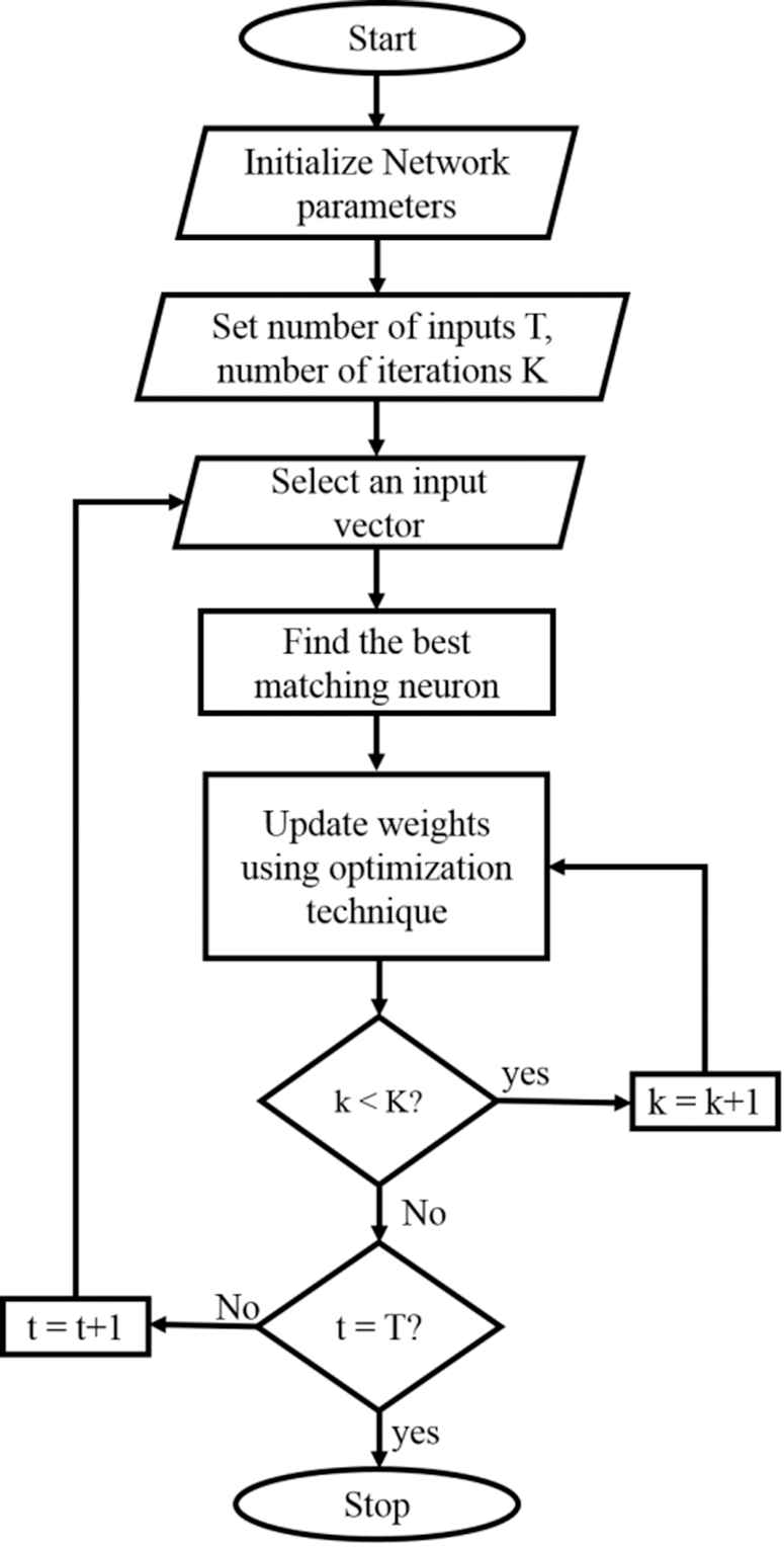
Flowchart of the hybrid self-organizing map (SOM).
The step by step procedure to implement Hybrid SOM classifier for iris recognition is as follows:
Step 1: Divide the given iris dataset into a training set and testing set.
Step 2: The feature vectors are computed from the iris images of the training set and given as input to the SOM network.
Step 3: Euclidean distance is measured between the input feature vector and all the output nodes. The nodes which are close to the input vector is termed as the winning node.
Step 4: All the neurons of the winner node are tweaked using metaheuristic optimization technique.
Step 5: Step 4 is repeated until the stopping condition is reached.
Step 6: The same procedure is repeated for all other iris images from step 2.
Step 7: With the learned weights, the iris images of the test dataset are recognized into its respective class.
The learning rate of the SOM network is assumed as 0.9. After the stopping condition, not much significant changes in the weight update is observed.
The self-organizing map consists of many weights associated with the tensors that connect each of the neurons of the input layer to the neurons in the output layer. During the process of training these weights are updated such that the weights converges to obtain minimum error between the target class and the predicted class. However, in this unsupervised classifier there are no labelled data. Hence, the networks learns to group itself in order to map the feature vector of a certain class with its corresponding output node. The rate at which it learns to converge and amount of error incurred after learning are two crucial aspects for a machine learning model. The conventional model of self-organizing map classifier uses the Hebb's rule. The major drawback of using this method is, the network takes more than five hundred times the feature vector size to get trained. The other drawback is the classification accuracy of the unsupervised model is not acceptable. This gives a space for improvement. The conventional SOM structure is made hybrid by introducing optimization method into the learning process. This outruns the conventional model by converging faster. The jitters that happens during the search of best matching unit is reduced by modifying the learning algorithm of the network. This helps the network to learn with better precision. The modified hybrid self-organizing map is briefed in Algorithm 1.
Algorithm 1 Modified Hybrid Self-organizing Map Classifier Training
Require: T, K, input feature vectors, random weight matrix W of size M x N
1: for t = 1 to T
2:
3:
4: for k = 1 to K
5: Update the neurons of the winning node P using optimization
6: Compute the cost
7: end
8: return P
9: Update
10: end
Instead of iterating through the training process for other feature vectors, after finding the winning neuron it is updated for maximum count. The weight update of the winning neuron is done using optimization methods described in pseudo code 1 to 4.
5.1. Optimization Used in the Classifier
Optimization method has multiple degrees of freedom to learn the weights. This can be employed in training the ANN. In this work, four different optimization methods are experimented to train the weight of the SOM network. Some of these optimization methods are inspired from the basic physics laws, human behavior, herd of animals and also flock of birds.
5.1.1. Gravity search algorithm
Rashedi et al. [27] have proposed Gravity Search Algorithm. The Newton's law of gravity is based on the fact that every particle in the universe attracts each other particle with a force that is directly proportional to the product of their masses and inversely proportional to the square of the distance between them. The working of Gravity Search Algorithm (GSA) is based on this law. The solutions in the search space for this optimization method are called agents. The gravitational force acting on these agents cause the agents to move toward the heavier mass. Each agent is represented by its position, inertial mass, active gravitational mass and passive gravitational mass. The position of the agent indicates the solution to the problem. The force and acceleration acting on the agents navigate the agents toward the best solution. The illustration of GSA is given in Pseudo code 1.
Pseudo code 1: Update rule using Gravity Search Algorithm
Initialization: K, Pbest,
1:
2:
3:
4:
5:
6: If fitness of
then
7: P =
The initial values are given as G0 = 500, Magm = 1, Mpgm = 1, Mim = 1 and α = 2. The winning neuron during the excitation process is taken as the initial position of the weight vector. Later, the position of this vector is adapted in sequence of steps such that it learns the best position which best describes its target class. This process of learning the weight is done over a number of iteration till the cost function is minimum.
5.1.2. Teacher learning based optimization algorithm
Rao et al. [28] have proposed Teaching–Learning based optimization to attain a global solution to nonlinear problems. It is developed on the inspiration of teaching and learning. In a classroom, the influence of a teacher on the outcome of the learners in the class is very high. A good teacher can train learners effectively and give better results. This concept is exploited in implementing the Teaching-Learning Based Optimization (TLBO). Initially, formulate the problem and set the TLBO parameters. Read the initial position and update the best solution based on the value of cost function. With the teacher help, solutions are given in the teaching phase. Later, the learner proposes and refines the solution to get the global best solution. The framework of the teacher learner-based optimization technique is shown in pseudo code 2.
Pseudo code 2: Update rule using TLBO algorithm
Initialization:
1:
2:
3:
4: If fitness value of
assign
5:
where
6: If the fitness value of
assign
else
assign
7: If fitness value of
assign
The initial values are given as
5.1.3. Whale optimization algorithm
Mirjalili et al. [29] have proposed Grey Wolf Optimization. It uses the leadership hierarchy and hunting behavior of the grey wolves to locate the near best solution in the search space. It always moves and hunts in a pack. Each member in the pack has a hierarchy on how they operate. It can be classified as alpha, beta and delta. It assists in the hunting process. The alpha is the fittest and leader of the pack. Whereas beta is the second fittest in the pack and delta is the third fittest in the pack. It helps in moving toward the target. All the wolves encircle the target during hunting. It avoids local minima. It is intelligible, adaptive and does not need any derivative mechanism. The detailed framework of the Gray Wolf Optimization (GWO) algorithm is shown in pseudo code 3. During each iteration, the alpha, beta and delta wolves keep changing in accordance with the fitness of the wolf in the optimization problem.
Pseudo code 3: Update rule using WOA
Initialization:
1:
2:
3: If
If
Then
if
Then D =
4: Else if
5: If fitness of
Then
The whales have the privilege of moving both in circular motion and linear motion on moving toward its best possible position. The node for which the dot product is maximum is taken as the winning node. The neurons of the winning node are assumed as the present position of the weight vector. Later, with the perception of the whale the weights move toward the best fitting position that describes the input feature with its respective class.
5.1.4. Grey wolf optimization
The hierarchy of wolves and their hunting behavior helps the search agent to reach near the target [30]. As the level of hierarchy is more, their contribution in identifying the optimal solution is more. This helps to attain the approximate solution. The step by step procedure for the GWO based Hybrid SOM classifier for iris recognition is shown in pseudo code 4. The hierarchy of the wolves are alpha, beta, delta and omega. The alpha, beta and delta are the ones who are best in their travel position toward the prey. The omega is the least powerful and has to obey and move with the information of alpha, beta and delta. Thus the omega converges with the best position over a number of iteration over which it trains the weights.
Pseudo code 4: Update rule using GWO
Initialization:
1:
2:
3:
4:
The initial values of the variables are given as
6. EXPERIMENTAL RESULTS AND DISCUSSIONS
This section describes the experimental results of the hybrid SOM classifier optimized with techniques namely gravity search algorithm, teacher–learner based optimization, whale optimization algorithm and grey wolf optimization. The experiments are conducted on iris images from IIT Delhi captured in infrared spectrum. Around 600 images are taken for training the models and a similar 150 images are taken for testing it. The algorithm is implemented on personal computer with 1.7 GHz clock and 4GB RAM. The simulations are done using preinstalled MATLAB (version 9.3, R2017b). The table describing the performance measures of results obtained on ten different classes averaged over five times. The results of the proposed model is validated with the confusion matrix and the performance measures calculated from it.
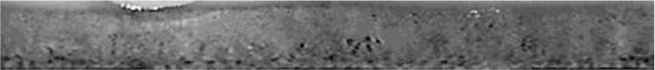
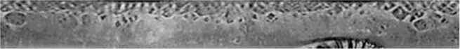
The iris image need to preprocessed to enhance the fine details of the captured iris image. In this work, contrast limited adaptive histogram equalization is used to enhance the iris image. Iris image enhancement will support more in further process to correctly locate the iris and pupil boundary. The enhanced iris images are given in Figure 5.

Iris image enhancement (a) nonuniform illuminated input image, (b) Contrast Limited Adaptive Histogram Equalization (CLAHE) enhanced iris image.

Iris localization (a) Iris and pupil boundary detected using Circular Hough Transform (CHT) (b) Segmented iris region.
To define the boundary of the iris region, circular Hough transform is used. Later, the region within the iris is extracted using appropriate mask. The localized iris done using circular hough transform is given in Figure 6.
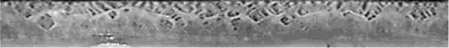
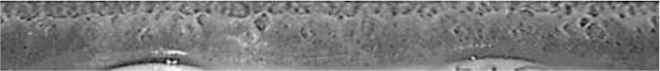
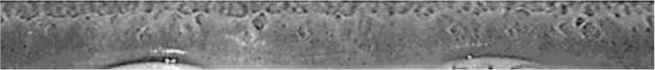
The exposure of the eye to light may vary the circular segmented iris region. To fix this irregularity, the segmented iris region is normalized using rubber sheet normalization. This transforms the circular region into a rectangular block of fixed size. Seven different statistical elements namely mean, SD, SM, RMS, E, S and K are extracted to form feature vector. These information are detailed in Table 1.
| Normalized Iris Image | Feature Vectors |
||||||
|---|---|---|---|---|---|---|---|
| Mean | SD | SM | RMS | E | S | K | |
 |
10.563 | 1.728 | 6.109 | 1.728 | 9.948 | 0.378 | 19.775 |
 |
15.427 | 1.135 | 13.581 | 2.578 | 8.725 | 0.206 | 14.785 |
 |
17.235 | 2.102 | 8.196 | 3.161 | 10.533 | 0.520 | 12.023 |
 |
6.823 | 0.968 | 7.046 | 0.868 | 7.347 | 0.911 | 10.994 |
 |
23.194 | 5.125 | 4.525 | 25.192 | 20.678 | 1.569 | 43.562 |
Normalized iris image and feature vector.
6.1. Performance Analysis of GSA Based Hybrid SOM Classifier
The results obtained over the classification problem can be contained within a confusion matrix. The key aspect of this matrix is that it gives the count values of correct and incorrect predictions tabulated across each class. The uncertainties of the network model during classification can be understood from the matrix. The count values of the successful and unsuccessful predictions are tabulated under true positives (TP), true negatives (TN), false positive (FP) and false negative (FN). The number of images that are correctly classified into its respective classes are labelled as TP. The number of uncertain classification that are misclassified are labelled as TN. The number of classifications for which images of certain class that is misclassified as other are labelled as FN. The number of classifications for which the images that do not belong to a particular class being predicted as that class itself are labelled as FP.
The count values of ten different classes is tabulated in the Tables 2–5 for reference. The Table 2 gives the outcome of the classification by hybrid SOM classifier with GSA. It can be seen from the table, that images of class 7 has large uncertainties and affects the performance of the classifier. The ability to solve nonlinear problems is greatly supported by GSA. The learning rate of the classifier is a decreasing function and hence can avoid settling for local minima.
| CLASS | TP | TN | FP | FN |
|---|---|---|---|---|
| Class 1 | 14 | 107 | 1 | 1 |
| Class 2 | 10 | 111 | 0 | 5 |
| Class 3 | 11 | 110 | 7 | 4 |
| Class 4 | 14 | 107 | 3 | 1 |
| Class 5 | 12 | 109 | 4 | 3 |
| Class 6 | 13 | 108 | 1 | 2 |
| Class 7 | 8 | 113 | 1 | 7 |
| Class 8 | 14 | 107 | 6 | 1 |
| Class 9 | 11 | 110 | 1 | 4 |
| Class 10 | 14 | 107 | 6 | 2 |
FN, false negative; FP, false positive; SOM, self-organizing map; TN, true negative; TP, true positive.
Performance measures of hybrid SOM classifier with GSA.
| CLASS | TP | TN | FP | FN |
|---|---|---|---|---|
| Class 1 | 14 | 117 | 1 | 1 |
| Class 2 | 10 | 121 | 0 | 5 |
| Class 3 | 11 | 120 | 4 | 4 |
| Class 4 | 14 | 117 | 3 | 1 |
| Class 5 | 15 | 116 | 3 | 0 |
| Class 6 | 14 | 117 | 1 | 1 |
| Class 7 | 12 | 119 | 1 | 3 |
| Class 8 | 15 | 116 | 5 | 0 |
| Class 9 | 12 | 119 | 0 | 3 |
| Class 10 | 14 | 117 | 2 | 2 |
FN, false negative; FP, false positive; SOM, self-organizing map; TN, true negative; TP, true positive.
Performance measures of hybrid SOM classifier with TLBO.
| CLASS | TP | TN | FP | FN |
|---|---|---|---|---|
| Class 1 | 15 | 121 | 0 | 0 |
| Class 2 | 12 | 124 | 0 | 3 |
| Class 3 | 11 | 125 | 4 | 4 |
| Class 4 | 15 | 121 | 2 | 0 |
| Class 5 | 15 | 121 | 1 | 0 |
| Class 6 | 15 | 121 | 0 | 0 |
| Class 7 | 12 | 124 | 1 | 3 |
| Class 8 | 15 | 121 | 5 | 0 |
| Class 9 | 12 | 124 | 0 | 3 |
| Class 10 | 14 | 122 | 2 | 2 |
FN, false negative; FP, false positive; SOM, self-organizing map; TN, true negative; TP, true positive.
Performance measures of hybrid SOM classifier with WOA.
| CLASS | TP | TN | FP | FN |
|---|---|---|---|---|
| Class 1 | 15 | 131 | 0 | 0 |
| Class 2 | 15 | 131 | 0 | 0 |
| Class 3 | 14 | 132 | 1 | 1 |
| Class 4 | 15 | 131 | 2 | 0 |
| Class 5 | 15 | 131 | 0 | 0 |
| Class 6 | 15 | 131 | 0 | 0 |
| Class 7 | 14 | 132 | 0 | 1 |
| Class 8 | 14 | 132 | 1 | 1 |
| Class 9 | 15 | 131 | 1 | 0 |
| Class 10 | 14 | 132 | 0 | 2 |
FN, false negative; FP, false positive; SOM, self-organizing map; TN, true negative; TP, true positive.
Performance measures of hybrid SOM classifier with GWO.
6.2. Performance Analysis of TLBO Based Hybrid SOM Classifier
The count values of the experiment on hybrid SOM classifier with TLBO is given in Table 3.
Relatively high jitters in classification of images under class 2 can be seen from the values in the above table. It is a metaheuristic search method inspired by the teaching–learning process in the classroom. The learner comes up with new possible solution from the instruction from the teacher. The solution learned by the learner is then validated with the best results. The learning phase of the hybrid network model is facilitated by this optimization method. The key advantage of this method is it does not need much of parameters to help in the optimization process.
6.3. Performance Analysis of WOA Based Hybrid SOM Classifier
The classification outputs of the hybrid SOM classifier with WOA is tabulated in Table 4.
Class 3 shows more uncertainties and affects the performance of the classifier. Starting with a random solution the algorithm converges to the best possible position in the search space. The instincts of the whale make it to move in spiral and linear motion makes it achieve the task. This has enable it to reduce the uncertainties.
6.4. Performance Analysis of GWO Based Hybrid SOM Classifier
The classification results of the HSOM classifier with GWO is tabulated in Table 5.
The classification results of the HSOM classifier with GWO is tabulated in Table 5. The uncertainties are minimized. This significantly improves the performance of the classifier. The hierarchical approach of GWO has three degrees of freedom, which makes better convergence than other methods. There are many metrics that validate the robustness of the classifier model. It tells about what fraction of the total input test images tested where predicted correctly. When the accuracy score is high it seems like a good classifier. Sensitivity is metric which gives the idea, how many images of a particular class is being correctly classified as itself out of all other classifications. This can be computed from the values of the confusion matrix. It is the actual correct classification. So if the FNs is reduced, it is sure that the all the images of a certain class is correctly classified. Specificity is measure that gives information about how much of an image not belonging to a class was correctly classified as the other class. In other words it the vice versa of sensitivity. For a robust classifier it is desired have a higher specificity score. This can be achieved by minimizing FPs. Positive prediction value is also termed as precision. In gives the fraction of a particular that is perfectly classified. Minimizing FPs can improve the precision of a model. Negative prediction value is the ratio of TN that were actually negatives.
As accuracy alone cannot assess the performance of the classifier, the best method to know which classifier performs better is by having a comparative analysis. Performance measures like sensitivity, specificity, positive predictive value (PPV), negative predictive value (NPV), false negative rate (FNR), false positive rate (FPR), area under curve (AUC), equal error rate (EER) and Gini impurity are used to compare the performance the proposed methods.
It can be seen from the Table 6 that, in terms of all performance metrics hybrid classifier with GWO performance better. This is because of the hierarchy in the searching process which gives maximum degrees of freedom. FNR is the miss rate. It gives the ratio of the images that are wrongly classified. The FPR is the false alarm ratio. It gives the ratio of images of other class being wrongly classified as a particular class. The behavior of a classifier model to a certain threshold can be studied with the help of receiver operating characteristic curve. Area under the curve is the entire area that is enclosed below the receiver operating characteristic curve. It gives a true performance of the model that can be effectively implemented in real-time. EER is the equal error rate which give the threshold value at which false acceptance rate is equal to false rejection rate. For better performance, it is preferred to have a low EER value for a classifier model. The Gini coefficient is calculated from the AUC. It describes the robustness of the classifier in random prediction.
| Accuracy | Sensitivity | Specificity | PPV | NPV | FNR | FPR | AUC | EER | Gini | |
|---|---|---|---|---|---|---|---|---|---|---|
| HSOM + GSA | 96.03 | 73.3 | 99.09 | 0.91 | 0.96 | 0.47 | 0.17 | 0.78 | 0.32 | 0.56 |
| HSOM + TLBO | 97.05 | 86.7 | 98.3 | 0.88 | 0.98 | 0.45 | 0.11 | 0.87 | 0.28 | 0.72 |
| HSOM + WOA | 97.8 | 90.8 | 98.8 | 0.91 | 0.98 | 0.37 | 0.08 | 0.91 | 0.22 | 0.82 |
| HSOM + GWO | 99.3 | 96.7 | 99.6 | 0.96 | 0.99 | 0.3 | 0.03 | 0.96 | 0.16 | 0.92 |
AUC, area under curve; EER, equal error rate; FNR, false negative rate; FPR, false positive rate; HSOM, hybrid self-organizing map; NPV, negative predictive value; PPV, positive predictive value.
Performance measures.
| Author | Method | Accuracy |
|---|---|---|
| Liu et al. | F-CNN | 81.4 |
| Pillai et al. | Kernal learning | 86.87 |
| Liu et al. | F-capsule | 83.3 |
| Oktiana et al. | Integrated gradient face | 95.69 |
| Proposed method 1 | HSOM + GSA | 96.03 |
| Proposed method 2 | HSOM + TLBO | 97.05 |
| Proposed method 3 | HSOM + WOA | 97.8 |
| Proposed method 4 | HSOM + GWO | 99.3 |
HSOM, hybrid self-organizing map.
Comparative analysis.
The accuracy of the proposed classifier is compared with some state-of-art classifiers to show its versatility. WOA and GWO are swarm intelligence based optimization methods. Since these operates in swarms they have higher degrees of freedom in exploring the best weights during the learning phase. The increased level of hierarchy has increased the intelligence of the hybrid SOM classifier. Hence, the accuracy of the hybrid classifier with GWO performs better than other methods. The GSA and TLBO based have relatively limited number of freedom compared to swarm-based optimization. Hence, they show relatively lesser accuracy.
Table 7 shows that the hybrid classifier with GWO outperforms all other methods. The organization behavior of the GWO helps in significant improvement in the performance measures of the classifier. The optimization methods help in updating the weights such that the feature vectors are able to correctly classify into its respective class. This update happens over a number of iterations till the error is minimum. Faster the convergence, lesser would be the time required for the classifier to learn the features.
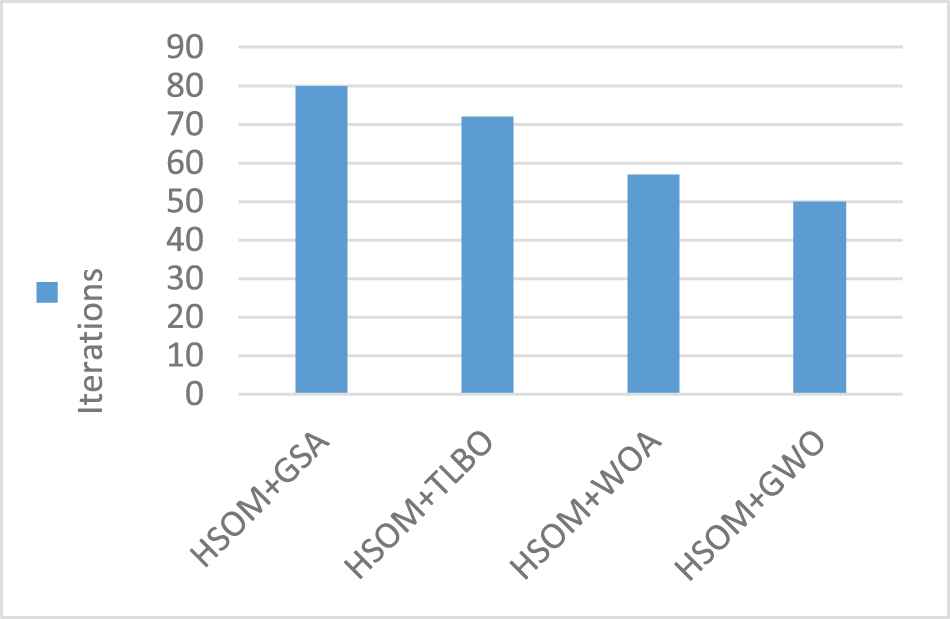
Number of iterations.
The Figure 7 show the number of iterations required by all the discussed methods in the training phase of the network model. For the hybrid classifier, GSA takes 80 iterations, TLBO takes 72 iterations, WOA takes 57 iterations and GWO takes 50 iterations for convergence. The iterations is the number of trainings taken for the cost function to be less than 10−3. This shows that the GWO optimizer is robust in training the network model and helps in faster convergence. It can be observed from the experimental results, that the introduction of optimization in the learning phase of the network model significantly improves the performance measures of the classifier. Overall, the proposed hybrid approach has better learning capability than the conventional approach because of it increased degree of freedom in learning the weights.
7. CONCLUSION AND FUTURE WORK
The focus of this work is to build a hybrid model to improve the performance of the iris biometrics. The success of the proposed method can be verified from the performance metrics of the experiments. It can be inferred that the swarm-based optimization helps in building a classifier model with better accuracy and faster convergence. This method discussed above have taken precaution like preprocessing to improve the image quality of the iris images enrolled with the system. This address the problem of low contrast and uneven distribution of contrast in the captured image due to poor illumination. However, there are certain other important factors which are not considered. Factors like blurring, occlusions due to eyelids and eyelashes which can affect the performance of the system. If these artefacts are addressed, proposed method can be more robust. It can improve the suitability to unconstrained environment. In spite of that, this algorithm shows favorable potential to incorporate iris biometric systems in real-time.
CONFLICT OF INTEREST
Authors have no conflict of interest to declare.
AUTHORS' CONTRIBUTIONS
J. Jenkin Winston - Analysis, Gul Fatma Tucker - Methodology, Utku Kose - Results Validation, D. Jude Hemanth - Analysis.
REFERENCES
Cite this article
TY  - JOUR
AU  - J. Jenkin Winston
AU  - Gul Fatma Turker
AU  - Utku Kose
AU  - D. Jude Hemanth
PY  - 2020
DA  - 2020/08/06
TI  - Novel Optimization Based Hybrid Self-Organizing Map Classifiers for Iris Image Recognition
JO  - International Journal of Computational Intelligence Systems
SP  - 1048
EP  - 1058
VL  - 13
IS  - 1
SN  - 1875-6883
UR  - https://doi.org/10.2991/ijcis.d.200721.001
DO  - 10.2991/ijcis.d.200721.001
ID  - Winston2020
ER  -