
Comparison of Recent Metaheuristic Algorithms for Shape Detection in Images
 , Angel Trujillo, Mario A. Navarro, Primitivo Diaz
- DOI
- 10.2991/ijcis.d.200729.001How to use a DOI?
- Keywords
- Metaheuristics; Shape detection; Image processing; Machine learning
- Abstract
Shape recognition in images represents one of the complex and hard-solving problems in computer vision due to its nonlinear, stochastic and incomplete nature. Classical image processing techniques have been normally used to solve this problem. Alternatively, shape recognition has also been conducted through metaheuristic algorithms. They have demonstrated to have a competitive performance in terms of robustness and accuracy. However, all of these schemes use old metaheuristic algorithms as the basis to identify geometrical structures in images. Original metaheuristic approaches experiment several limitations such as premature convergence and low diversity. Through the introduction of new models and evolutionary operators, recent metaheuristic methods have addressed these difficulties providing in general better results. This paper presents a comparative analysis on the application of five recent metaheuristic schemes to the shape recognition problem such as the Grey Wolf Optimizer (GWO), Whale Optimizer Algorithm (WOA), Crow Search Algorithm (CSA), Gravitational Search Algorithm (GSA) and Cuckoo Search (CS). Since such approaches have been successful in several new applications, the objective is to determine their efficiency when they face a complex problem such as shape detection. Numerical simulations, performed on a set of experiments composed of images with different difficulty levels, demonstrates the capacities of each approach.
- Copyright
- © 2020 The Authors. Published by Atlantis Press B.V.
- Open Access
- This is an open access article distributed under the CC BY-NC 4.0 license (http://creativecommons.org/licenses/by-nc/4.0/).
1. INTRODUCTION
The problem of shape detection such as lines, circles, circular arcs and ellipses appears in several fields of pattern recognition with uses in many industrial applications from automatic object recognition to car navigation [1]. Shape detection is normally conducted through the Hough Transform (HT) [1,2]. A standard Hough-based scheme uses edge information produced by an edge detector algorithm to obtain candidate geometrical shapes. In the process, each edge pixel, which coincides with a hypothetical geometrical shape, votes in the parameter space with the information that corresponds to its parameters. Then, the most probable shape is obtained by averaging, filtering and histogramming the parameter space. HT is a robust algorithm; however, it maintains some important flaws. HT requires a large amount of space to store all considered parameters of the geometrical shape. It also needs a high computational complexity, which yields a low performance in terms of speed. Another critical problem is accuracy. In HT, the precision of the obtained parameters for the detected shape is reduced, especially in noise conditions [3].
Alternatively to the HT, the problem of shape detection has also been faced through metaheuristic approaches. In general terms, they have shown better results than those that use the HT concerning accuracy, speed and robustness [4]. A detector, based on a metaheuristic scheme, utilizes a set of edge points as decision variables to determine hypothetical shapes (possible solutions). A matching function evaluates if a hypothetical shape is actually contained in the image. Therefore, conducted by the values of the matching function, the set of encoded points are operated through a particular metaheuristic approach so that the best solutions represent the original shapes inside the image. Different pioneer metaheuristic algorithms have been used to produce several interesting shape detectors such as Genetic algorithms (GAs) [5,6] and Particle Swarm Optimization (PSO) [7], Differential Evolution (DE) [8], Cloning Selection method (CSM) [9], Harmony Search (HS) [10], Artificial Bee Colony (ABC) [11] and Animal Behavior (AB) [12,13].
Recently, metaheuristic approaches have consolidated their popularity with exceptional growth and a large number of applications [14]. Such approaches represent difficult opposition to classical optimization techniques, which are prone to fail in several simple contexts. On the other hand, initial metaheuristic schemes maintain in their design several limitations such as premature convergence and inability to maintain population diversity [15]. Recent metaheuristic methods have addressed these difficulties providing in general better results [16]. Many of these novel metaheuristic approaches have also been introduced lately. In general, they propose new models and innovative evolutionary operators for producing an adequate exploration and exploitation of large search spaces considering a significant number of dimensions. This new generation of metaheuristic approaches is large, some examples include Crow Search Algorithm (CSA) [17], Cuckoo Search (CS) [18], Moth-flame Optimization Algorithm (MFOA) [19], Grey Wolf Optimizer (GWO) [20], Whale Optimization Algorithm (WOA) [21], Gravitational Search Algorithm (GSA) [22], Sine Cosine Algorithm (SCA) [23], Cricket Behavior-Based Evolutionary (CBE) [24], Dragonfly Algorithm (DF) [25], Hybrid Cognitive Optimization Algorithm (HCOA) [26], Interactive Search Algorithm (ISA) [27], Farmland Fertility Algorithm (FFA) [28], Binary Artificial Algae Algorithm (BAAA) [29], Electro-Search algorithm (ESA) [30], Island Bat Algorithm for Optimization (IBAO) [31], to name a few.
According to the literature, there is no single metaheuristic scheme that can solve every problem effectively. Metaheuristic schemes have been designed with special search models that allow them to solve competitively specific problems. Under such conditions, to evaluate the performance of a certain metaheuristic method appropriately, its relative efficiency should be assessed in the scenario in which it would be applied. Different comparisons among metaheuristic methods have been presented in several studies where it is analyzed their solutions over a representative set of benchmark functions with exact solutions and well-known behaviors. However, their conclusions are limited since they do not consider any application context. This paper presents a comparative analysis on the application of five recent and most popular metaheuristic schemes to the shape recognition problem such as the GWO, Whale Optimizer Algorithm (WOA), CSA, GSA and CS. These algorithms have been successful in several new domains. Under this condition, the objective is to determine their efficiency when they face a complex problem such as shape detection. Such approaches have been selected for our analysis, since they are considered the methods most currently in use according to the popular scientific databases, ScienceDirect (http://www.sciencedirect.com), SpringerLink (http://www.springerlink.com) and IEEE Xplore (http://ieeexplore.ieee.org), over the last five years. The problem of shape detection involves the identification of lines, circles, circular arcs and ellipses. In this work, in order to provide an interesting comparison among all the methods, the ellipse detection has been selected. It is considered the most complex recognition task with regard to lines and circular features. The comparison is divided into two parts. In the first part, the performance of all metaheuristic algorithms is evaluated with regard to the ellipse detection in natural images, while, in the second part, the robustness in the detection of each algorithm in the presence of complex scenarios is analyzed. In the study, several performance indexes have been considered to evaluate the accuracy of detection and computational overload. Additionally, test methods are achieved over the experimental data in order to validate the results.
The remainder of this paper is organized as follows: Section 2 formulates the detection problem such as an optimization task; in Section 3 the main characteristic of each compared algorithms are presented; in Section 4, a comparative perspective of the involved metaheuristic schemes is analyzed; in Section 5, the numerical results are presented. Finally, in Section 6, conclusions are given.
2. PROBLEM FORMULATION
To identify ellipse in images, they must be firstly preprocessed by an edge detection algorithm that produces a single-pixel-contour edge map (such as the Canny method). Next, the location
| Pixel position of the edge element |
|
| Edge vector that contains all the edges presented in the image | |
| Total number of detected edge pixels in the image | |
| Ellipse candidate coded as the combination of five different edge points where |
|
| Coefficients that define the ellipse characteristics | |
| Normalized coefficients of the ellipse so that |
|
| Center of the ellipse | |
| Maximal radius and minimal radii, respectively. They correspond to the maximum axis and minimum axis | |
| Ellipse orientation | |
| Temporary variables, where |
|
| The determinant of the ellipse parameters so that |
|
| A hypothetical set of points that define the ellipse candidate |
|
| Number of hypothetical points that involve the ellipse candidate |
|
| Pixel position of each hypothetical point |
|
| Matching error of the candidate ellipse |
|
| Relation to decide if |
|
| Function that checks the existence of the ellipse perimeter point |
Description of each symbol used in this section.
In this scheme, a candidate solution
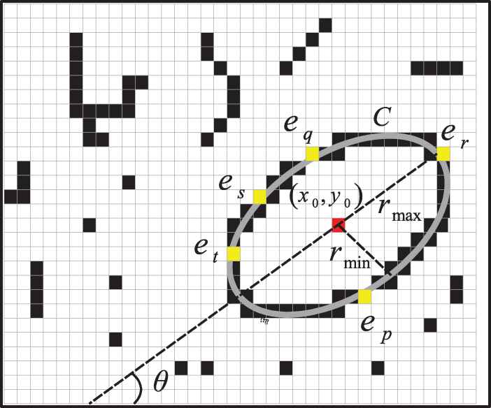
Candidate ellipse shape produced from the combination of points.
With this method, according to Figure 1, a candidate shape is represented as the ellipse which passes through the five points
Consequently, by replacing the coordinates of each parameter point
From this model, the main geometrical characteristics of the ellipse such as the center
To estimate the matching error
The set
Once determined the perimeter points
A value of
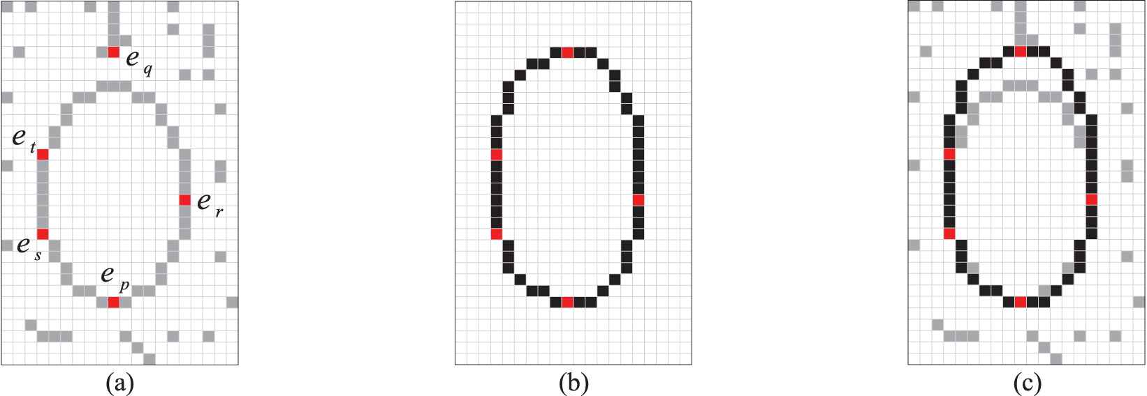
Computation of the matching error.
Figure 2(a) illustrates the original edge map
2.1. Multiple Ellipse Detection
To detect multiple instances, the shape detector stores the best ellipse candidate in each iteration
Once computed
3. OPTIMIZATION TECHNIQUES
Optimization methods have been devised to find the global solution
To find the best solution for Eq. (11), from a metaheuristic viewpoint [33], a group of
This section presents the main characteristics of the five metaheuristic optimization approaches used in the comparison the GWO, WOA, CSA, GSA and CS.
3.1. GWO Algorithm
The GWO [20] is a metaheuristic algorithm that models its search strategy considering the social hierarchy and hunting process conducted by wolves.
3.1.1. Hierarchy
To implement a mathematical model of the social hierarchy in the algorithm, the best candidate solution
3.1.2. Covering the prey
In Grey wolf packs, wolves try to encircle prey during their hunting behavior. This process is modeled as follows:
3.1.3. Hunting
In the hunting behavior, the search strategy is conducted mainly by the Alfa agent
3.1.4. Exploitation and exploitation
Both processes are implemented in the search strategy through the value of
3.2. Whale Optimizer Algorithm
The WOA [21] is an interesting metaheuristic method based on the particular spiral bubble-net hunting behavior found in humpback whales.
3.2.1. Encircling a prey
Under the WOA scheme, it is considered that the best candidate solution
3.2.2. Bubble-net attacking method
In this step, humpback whales use two procedures: shrinking (I) encircling and (II) spiraling. Both processes consider the modification of agent positions around the target element. In the approach, it is assumed that both procedures maintain an identical probability
3.3. Crow Search Algorithm
The CSA [17] is a metaheuristic approach inspired by the complex process presented in crows when they search for food resources. In CSA, each search agent
Under the CSA scheme, the location of each
(I) Pursuit. In this process, an agent
(II) Evasion. The agent
Each agent
3.4. Gravitational Search Algorithm
The GSA [22] is a metaheuristic approach inspired by the laws of gravitation. In GSA, the first step is to calculate the total gravitational force. It represents the influence that exerts the set of the best
Finally, the position of each agent is updated as follows:
3.5. CS Method
The CS [18] method is a metaheuristic algorithm for global optimization inspired by the behavior of cuckoo birds. Under the CS scheme, Levy flight random walk and biased random walk are employed as the basis for its search strategy. In a Levy flight random walk, a displacement is produced by sampling a Levy probability distribution which can be modeled as follows:
4. COMPARATIVE PERSPECTIVE OF THE FIVE METAHEURISTIC METHODS
The five metaheuristic methods used in this study: GWO, WOA, CSA, GSA and CS are based on different search mechanisms. In this section, a comparative perspective of these methods is analyzed. The discussion considers the observable properties of each metaheuristic algorithms and the way in which such characteristics present an effect in the performance of these schemes.
It is widely accepted in the metaheuristic community that a proper balance between exploration and exploitation determines the potential of a metaheuristic approach [34]. Exploration refers to the process of searching for new points of the solution space. On the other hand, exploitation represents the operation of polishing those previously visited solutions to improve their relative quality by using a local search mechanism. The use of the only exploration diminishes the accuracy of the solutions but raises the ability of the algorithm to obtain new promising solutions [35]. On the contrary, the application of exclusive exploitation allows increasing the precision of existing solutions. However, unfavorably provokes that the optimization process converges prematurely to locally optimal solutions [36]. The rate between exploration and exploitation experimented by a metaheuristic method depends on the mechanism of its search strategy.
In the analysis of the five metaheuristic methods, it has been considered the study of their search strategy and implementations. The search strategy has been divided into two different parts: selection approach or attraction scheme and independence on the evolution process.
The selection approach refers to the way in which each metaheuristic method collects solutions among the entire population to produce new ones. Such selected solutions are normally used as main elements to produce attraction operators in order to modify the positions of the current population. Basically, there exist two different schemes [34]: greedy, random and complete. Greedy selection considers the use of the best element or elements in terms of fitness values. Greedy selection ensures that most fitting individuals remain intact during the evolution process. Under such conditions, this scheme promotes the exploitation of the search space, increasing the fast convergence toward promising solutions. The algorithms GWO and WOA are considered within this category. The WOA uses the best individual (only one element) as an important element in its search strategy. In the case of the GWO method, it is remarkable that its selection mechanism uses the three best elements of the population. This fact allows not only favor exploitation but also increase diversity through the use of distinct solution types. On the other hand, random selection considers the use of an individual randomly selected within the complete population. The use of random elements promotes the exploration of the search space. However, adversely, it negatively affects to obtain consistent results or good accuracy. The algorithms CSA and CS consider the use of the random solution as part of their search strategy. Finally, the complete selection considers the use of all elements in the population to produce a new solution. This strategy uses, in general, the averaged position of all solutions to generate search direction patterns. This mechanism produces very low search schemes where it is necessary for an additional number of iterations to obtain the best optimization results. The GSA method uses the complete selection mechanism as in its search paradigm.
Regarding the independence of the evolution process [37], two different processes are distinguished: dependent and independent. Dependent processes represent strategies in which the number of iterations is considered to modify the search strategy. The idea under these schemes is to adapt the search strategy so that in the beginning, the exploration of the search space would be promoted while in the ending, the exploitation of the found solutions would be favored [38]. Representative schemes of this category are the GSA and CSA. Dependent methods present several difficulties since the results of the search process are not considering in the strategy; it is more important the number of iterations. Independent algorithms do not consider the stage of the evolution process to conduct their own search strategy. These algorithms use the knowledge produced by the obtained results to operate their search strategies [39]. In general terms, independent methods deliver better results than dependent methods. The algorithms GWO, WOA and CS are considered independent methods.
In terms of implementation, it is compared to the difficulty that represents the use and operation of each from the five metaheuristic methods. The algorithms are classified according to their implementation issues [R1] in low, medium and high. Such categories consider two factors: the number of configurable parameters and the extension of code necessary for its programming. The problem of parameter tuning depends on the number of configurable parameters [40]. It is important to remark that an appropriate configuration produces a correct balance between exploration and exploitation and thus, competitive results. Currently, there is no standard methodology that allows the proper setting of a metaheuristic scheme. In fact, researchers and practitioners configure the parameters of metaheuristics algorithms by hand, guided only by the process of trial and error. Under such circumstances, the GWO and WOA are the metaheuristic schemes that do not consider any parameter to calibrate. The CS and CSA use four parameters, while the GSA employs three elements. Among the five schemes presented in this study, some show a high level of simplicity so that they can be promptly translated onto computational code with relative easiness [41]. In contrast, others are relatively complex due to the behaviors and rules considered in the model. According to these levels, the extension of necessary code to implement a certain metaheuristic method can be used as a criterion to classified each scheme in simple and complex. Therefore, the GWO, WOA, CSA present a simple level of programming while CS and GSA maintain a complex programming model. According to their implementation, the algorithms considered in this analysis can be classified as follows: GWO and WOA as low, CSA as medium and CS and GSA as high. Table 2 summarizes all the comparative characteristics analyzed for each of the five algorithms.
| Algorithm | Search Strategy | Implementation | |
|---|---|---|---|
| Selection or Attraction Scheme | Independence on the Evolution Process | ||
| GWO | Greedy | Independent | Low |
| WOA | Greedy | Independent | Low |
| CSA | Random | Dependent | Medium |
| CS | Random | Independent | High |
| GSA | Complete | Dependent | High |
GWO, Grey Wolf Optimizer; WOA, Whale Optimizer Algorithm; CSA, Crow Search Algorithm; GSA, Gravitational Search Algorithm; CS, Cuckoo Search.
Comparative characteristics analyzed for each from the five algorithms.
5. EXPERIMENTAL RESULTS
An experimental analysis has been conducted with the objective of comparing the performance of all detectors. The experiments consider the capacity of each detector to recognize accurately ellipsoid shapes.
5.1. Performance Indexes
In the study, two performance indexes have been considered in the comparisons: the multiple error (
Images do not typically include perfect ellipses. Therefore, to examine the precision in the detection of a single ellipse, it is compared with a ground-truth ellipse that is obtained visually from the original image. In consequence, the parameters
In Eq. (34),
Metaheuristic approaches are, in general, complex programs with different operations and stochastic branches. Therefore, it is problematic, from a deterministic perspective, to develop a complexity analysis. As a result, the CT is considered to estimate the computational effort. Under this condition, CT expresses the CPU time spent by a metaheuristic scheme when it is under execution.
5.2. Experimental Comparison
In this subsection, the five metaheuristic schemes GWO [20], the WOA [21], the CSA [17], the GSA [22] and the CS [18] are compared in the detection of ellipses in digital images. The experiments consider even the capacity of each detector to recognize occluded or incomplete shapes such as arcs segments. In the analysis, the population size
The experimental results are divided into two parts. In Section 5.2.1, the performance of all metaheuristic algorithms is evaluated with regard to the ellipse detection in natural images. In Section 5.2.2, the robustness in the detection of each algorithm in the presence of complex scenarios is analyzed.
5.2.1. Detection in natural images
In comparison, all the five metaheuristic methods have been executed considering a fixed number of 1000 iterations (k = Maxgen). This stop criterion has been established to maintain compatibility with other similar works found in the literature [7–13]. To minimize the random influence in the results, each experiment is tested for 30 independent executions.
In the study, a representative set of four different images collected from the literature have been used. Figure 3 shows the complete set of images. In the figure, each image is labeled as D1.X that refers to the image X from experiment one. In the study, the ground-truth solutions for all images have been visually produced from their original versions.
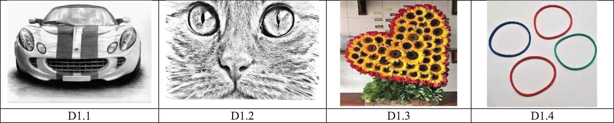
Set of natural images used to evaluate the performance of each metaheuristic algorithm.
The visual results in the application of all methods are depicted in Figure 4. Since every metaheuristic algorithm is executed 30 times over the same image, the detection results are presented in terms of the average
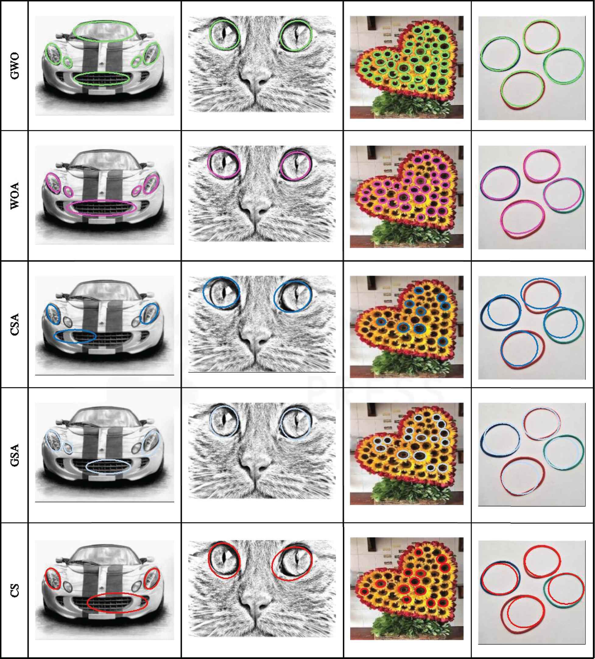
Visual results of the metaheuristic detectors over natural images.
According to Table 3, in terms of the average
| D1.1 | D1.2 | D1.3 | D1.4 | ||
|---|---|---|---|---|---|
| GWO | 0.2750 | 0.1991 | 0.1051 | 0.1679 | |
| 0.0220 | 0.0194 | 0.0067 | 0.0205 | ||
| WOA | 0.3245 | 0.2298 | 0.1185 | 0.1921 | |
| 0.0304 | 0.0404 | 0.0098 | 0.0205 | ||
| CSA | 0.9272 | 0.9250 | 0.9250 | 0.7793 | |
| 0.0591 | 0.0435 | 0.0421 | 0.0719 | ||
| GSA | 0.4913 | 0.4658 | 0.2509 | 0.2426 | |
| 0.0536 | 0.0435 | 0.0421 | 0.0719 | ||
| CS | 0.8442 | 0.6915 | 0.9381 | 0.9991 | |
| 0.0381 | 0.0536 | 0.0009 | 0.0001 |
GWO, Grey Wolf Optimizer; WOA, Whale Optimizer Algorithm; CSA, Crow Search Algorithm; GSA, Gravitational Search Algorithm; CS, Cuckoo Search; ME, Multiple Error.
Detection results of each metaheuristic algorithm for natural images.
Once identified the GWO approach as the best shape detection method, a nonparametric analysis known as the Wilcoxon test [42,43] has been achieved to validate this conclusion. The Wilcoxon analysis permits to assess the performance differences between two computing methods. The experiment is conducted for the 5% (0.05) significance level considering the
| GWO vs. WOA | GWO vs. CSA | GWO vs. GSA | GWO vs. CS | |
|---|---|---|---|---|
| D1.1 | 2.25E-04 ▲ | 8.76E-11 ▲ | 1.43E-09 ▲ | 4.84E-07 ▲ |
| D1.2 | 6.67E-03 ▲ | 5.32E-11 ▲ | 3.97E-09 ▲ | 7.73E-07 ▲ |
| D1.3 | 5.08E-01 ► | 2.01E-11 ▲ | 6.28E-09 ▲ | 1.09E-07 ▲ |
| D1.4 | 9.33E-02 ► | 3.22E-11 ▲ | 9.43E-10 ▲ | 8.05E-08 ▲ |
GWO, Grey Wolf Optimizer; WOA, Whale Optimizer Algorithm; CSA, Crow Search Algorithm; GSA, Gravitational Search Algorithm; CS, Cuckoo Search; ME, Multiple Error.
p-values generated by Wilcoxon analysis associating GWO vs. WOA, GWO vs. CSA, GWO vs. GSA and GWO vs. CS over the ME of 30 different executions (natural images).
According to the results from Table 4, it is clear that all p-values in the GWO vs. CSA, GWO vs. GSA and GWO vs. CS columns are less than 0.05 (5% significance level) which is sufficient evidence against the null hypothesis indicating that the GWO algorithm maintains a better (▲) performance than the CSA, GSA and CS methods. The result of the Wilcoxon analysis establishes that the conclusion is statistically significant, which means that it has not happened because of the usual noise included in the experimental data. In the case of the images D1.3 and D1.4, the GWO approach presents a similar performance as the WOA scheme. This conclusion is observed from the column GWO vs. WOA, where the p-values of such images are higher than 0.05 (►). Under these conditions, there is no statistical difference regarding the performance between both methods. As a summary, the results of the Wilcoxon test confirm that the GWO method performs better than other approaches under analysis.
The comparison of the final average
According to the results of Table 5, the CSA method obtain the best
| D1.1 | D1.2 | D1.3 | D1.4 | |
|---|---|---|---|---|
| GWO | 37.42 | 41.9 | 65.67 | 67.21 |
| WOA | 40.53 | 38.2 | 74.14 | 70.12 |
| CSA | 10.98 | 21.07 | 30.54 | 40.87 |
| GSA | 73.05 | 51.14 | 87.25 | 92.47 |
| CS | 85.12 | 67.29 | 97.18 | 128.14 |
GWO, Grey Wolf Optimizer; WOA, Whale Optimizer Algorithm; CSA, Crow Search Algorithm; GSA, Gravitational Search Algorithm; CS, Cuckoo Search; CT, Computational Time.
Average CT¯ in seconds for each metaheuristic detector for natural images.
5.2.2. Detection in complex scenarios
In this experiment, it is discussed the ability of each metaheuristic method to find suitable solutions in case of imperfect ellipses such as hand-drawn shapes or under noise conditions. This functionality is relevant since this problem appears typically in computer vision and image processing. In this paper, the ellipse detection problem has been conceived as an optimization task. Then, each metaheuristic method tries to find the best ellipse that matches a given shape under different conditions according to the objective function values
In the experiments, all metaheuristic algorithms have been executed considering a fixed number of 1000 iterations (k = Maxgen). Each experiment is tested for 30 independent executions in order to minimize the random influence in the results. In the analysis, a representative set of four different images collected from the literature have been used. Figure 5 shows the complete set of images. In the figure, each image is labeled as D2.X that refers to the image X from experiment two. In the study, the ground-truth solutions for all images have been visually produced from their original versions.
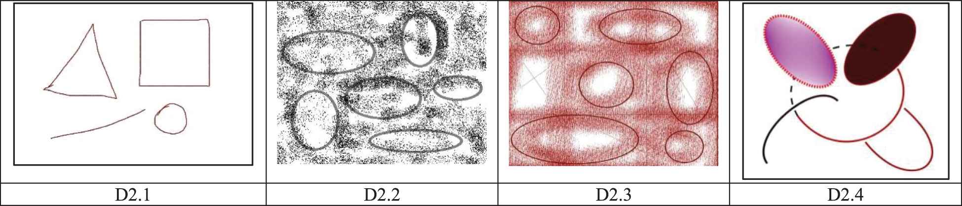
Set of images used to evaluate the performance of each metaheuristic algorithm under complex detection scenarios.
The visual results in the application of all methods are depicted in Figure 6. Since every metaheuristic algorithm is executed 30 times over the same image, the detection results are presented in terms of the average
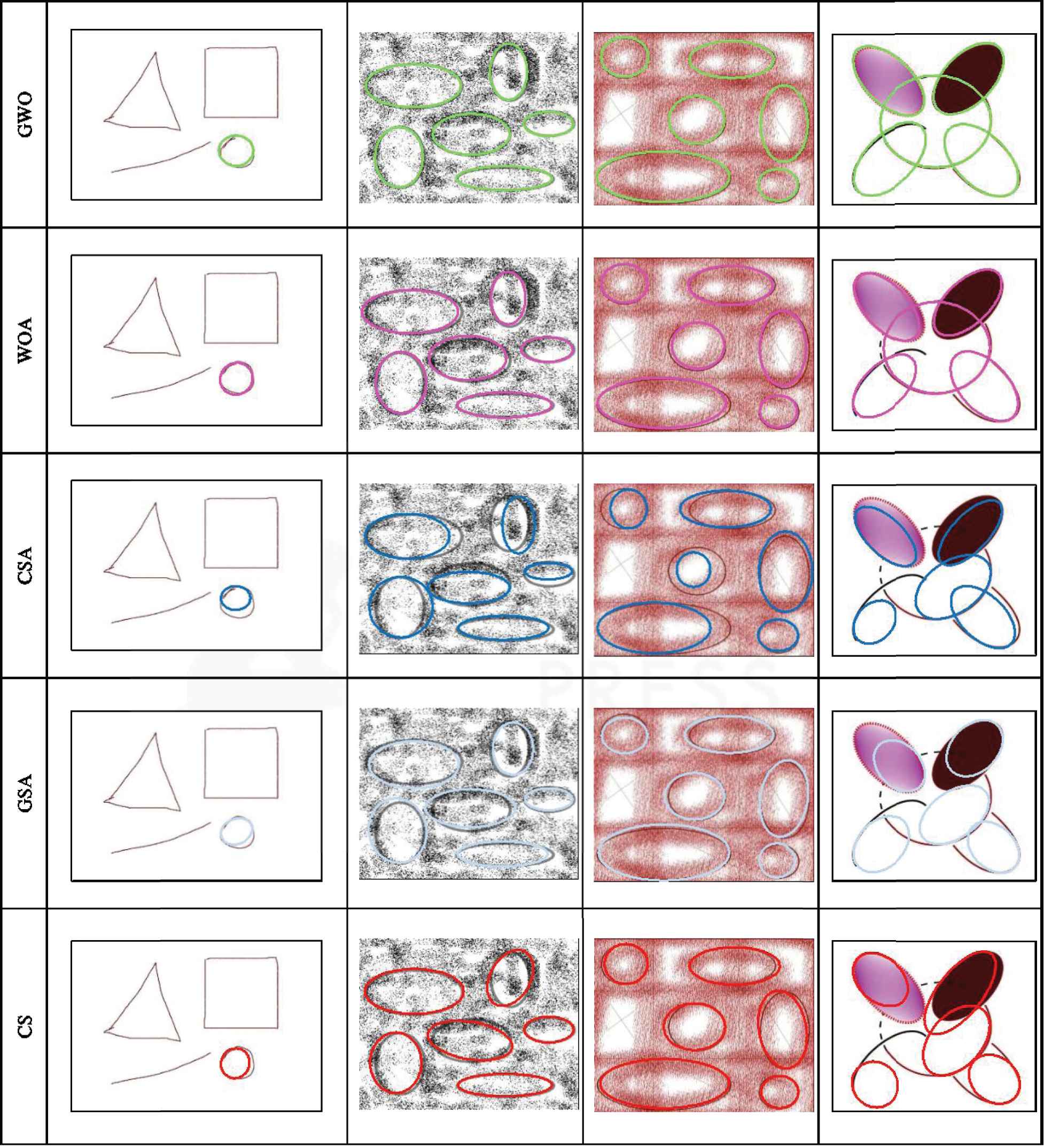
Visual results of the metaheuristic methods in the detection of complex scenarios.
| D2.1 | D2.2 | D2.3 | D2.4 | ||
|---|---|---|---|---|---|
| GWO | 0.5388 | 0.09859 | 0.2974 | 0.3454 | |
| 0.0215 | 0.0368 | 0.7253 | 0.0193 | ||
| WOA | 0.5494 | 0.2298 | 0.1185 | 0.1921 | |
| 0.0335 | 0.0385 | 1.2178 | 0.0208 | ||
| CSA | 0.9225 | 0.8180 | 0.9790 | 0.9140 | |
| 0.0514 | 0.0984 | 1.5961 | 0.0507 | ||
| GSA | 0.7072 | 0.1779 | 0.6915 | 0.4911 | |
| 0.0361 | 0.0488 | 1.3925 | 0.0570 | ||
| CS | 0.8012 | 0.2813 | 0.4494 | 0.6330 | |
| 0.0157 | 0.0225 | 0.4781 | 0.0313 |
GWO, Grey Wolf Optimizer; WOA, Whale Optimizer Algorithm; CSA, Crow Search Algorithm; GSA, Gravitational Search Algorithm; CS, Cuckoo Search; ME, Multiple Error.
Detection results of each metaheuristic algorithm for natural images.
According to Table 6, the advantage of the GWO over CSA, GSA and CS is also confirmed in terms of the
As a consequence, it is possible to find the best possible ellipse detection, even in complex conditions. This effect can be verified by the
The validation results of the Wilcoxon test for the detection of complex scenarios are presented in Table 7. They register the
| GWO vs. WOA | GWO vs. CSA | GWO vs. GSA | GWO vs. CS | |
|---|---|---|---|---|
| D2.1 | 8.24E-02 ► | 3.02E-11 ▲ | 5.64E-07 ▲ | 3.21E-08 ▲ |
| D2.2 | 6.73E-01 ► | 1.41E-11 ▲ | 2.88E-10 ▲ | 4.46E-08 ▲ |
| D2.3 | 2.40E-01 ► | 4.98E-11 ▲ | 2.97E-10 ▲ | 5.10E-08 ▲ |
| D2.4 | 7.95E-03 ▲ | 1.54E-11 ▲ | 7.18E-11 ▲ | 6.38E-09 ▲ |
GWO, Grey Wolf Optimizer; WOA, Whale Optimizer Algorithm; CSA, Crow Search Algorithm; GSA, Gravitational Search Algorithm; CS, Cuckoo Search; ME, Multiple Error.
p-values generated by Wilcoxon analysis associating GWO vs. WOA, GWO vs. CSA, GWO vs. GSA and GWO vs. CS over the ME of 30 different executions (detection in complex scenarios).
To extend the performance analysis of each metaheuristic algorithm, the CT invested by them over images in complex scenarios has also been conducted. Table 8 presents the average
| D1.1 | D1.2 | D1.3 | D1.4 | |
|---|---|---|---|---|
| GWO | 29.49 | 6.87 | 7.39 | 21.95 |
| WOA | 32.41 | 8.51 | 8.24 | 24.37 |
| CSA | 9.41 | 2.74 | 1.76 | 10.03 |
| GSA | 37.21 | 12.87 | 10.52 | 29.97 |
| CS | 35.23 | 11.43 | 10.87 | 27.08 |
GWO, Grey Wolf Optimizer; WOA, Whale Optimizer Algorithm; CSA, Crow Search Algorithm; GSA, Gravitational Search Algorithm; CS, Cuckoo Search; CT, Computational Time.
Average CT¯ in seconds for each metaheuristic detector for complex scenarios.
6. CONCLUSIONS
In this paper, a comparative analysis of the application of five recent metaheuristic schemes to the shape recognition problem has been presented. In the study, the GWO, WOA, CSA, GSA and CS have been considered. These algorithms have been successful in several new domains. Under this condition, the objective is to determine their efficiency when they face a complex problem such as shape detection.
In order to provide an interesting comparison among all the methods, the ellipse detection has been selected. It has been considered the most complex recognition task with regard to lines and circular features. The comparison is divided into two parts. In the first part, the performance of all metaheuristic algorithms is evaluated with regard to the ellipse detection in natural images, while, in the second part, the robustness in the detection of each algorithm in the presence of complex scenarios is analyzed. In the study, several performance indexes have been considered to evaluate the accuracy of the detection and computational overload.
The results demonstrated that the GWO obtained the best performance indexes in comparison with the other approaches. This conclusion has been statistically validated according to the Wilcoxon test.
CONFLICTS OF INTEREST
The authors declare that there are no conflicts of interest regarding the publication of this paper.
AUTHORS' CONTRIBUTIONS
The authors have contributed to all processes and stages of this research.
Funding Statement
This research has not been found for any institution.
REFERENCES
Cite this article
TY  - JOUR
AU  - Erik Cuevas
AU  - Angel Trujillo
AU  - Mario A. Navarro
AU  - Primitivo Diaz
PY  - 2020
DA  - 2020/08/05
TI  - Comparison of Recent Metaheuristic Algorithms for Shape Detection in Images
JO  - International Journal of Computational Intelligence Systems
SP  - 1059
EP  - 1071
VL  - 13
IS  - 1
SN  - 1875-6883
UR  - https://doi.org/10.2991/ijcis.d.200729.001
DO  - 10.2991/ijcis.d.200729.001
ID  - Cuevas2020
ER  -