
Flow Measurement of Natural Gas in Pipeline Based on 1D-Convolutional Neural Network
- DOI
- 10.2991/ijcis.d.200803.002How to use a DOI?
- Keywords
- Flow measurement; Ultrasonic signal; Arrival time; Feature recognition; Convolutional neural network
- Abstract
Time-difference method is a vitally significant algorithm for measuring natural gas flow with ultrasonic gas flowmeter. The key of this algorithm is to accurately measure the arrival time of ultrasonic signal. However, it is difficult to determine the feature points corresponding to the arrival time stably and accurately. To solve this problem, based on great feature recognition ability of deep learning, one-dimensional-convolutional neural network (1D-CNN) is utilized to determine the arrival time of ultrasonic signal according to the feature of the arrival time. First of all, a dataset, which includes different features such as different arrival time, different signal-to-noises (SNRs), etc., is used as a training set to train the 1D-CNN. Then, based on the size of the training set, an 1D-CNN is designed which includes three convolution and pooling layers and one fully connected layer to determine the arrival time, and the gas flow rate is calculated. To verify this method, an experimental ultrasonic gas flowmeter system is developed. By comparing with the typical method of determining arrival time, most of the deviations distribute close to zero and less than ±5 us using the proposed 1D-CNN, which verifies the effectiveness of the proposed 1D-CNN method.
- Copyright
- © 2020 The Authors. Published by Atlantis Press B.V.
- Open Access
- This is an open access article distributed under the CC BY-NC 4.0 license (http://creativecommons.org/licenses/by-nc/4.0/).
1. INTRODUCTION
As green clean, environment-friendly energy, natural gas is widely used in various fields of production activities [1]. In the power industry, natural gas can replace coal for power generation, which can reduce environmental pollution and obtain low-cost power [2]. In the chemical industry, natural gas is the best raw material to produce nitrogen fertilizer, which has the characteristics of less investment, low cost and less pollution [3]. And natural gas can replace gasoline as the driving energy of vehicle [4]. Because of China's vast territory, the main mode of natural gas transportation is pipeline transportation which can reduce transportation costs effectively, improve the efficiency of transportation of natural gas and realize automatic control of the transportation. In natural gas pipeline transportation, the automatic monitoring of gas flow is the core. Nowadays, various gas flow meters are used to measure natural gas flow, such as orifice gas flowmeter [5], vortex gas flowmeter [6], ultrasonic gas flowmeter [7]. The orifice flowmeter has the advantages of high reliability, convenient processing and installation, small measuring range and large pressure drop. Vortex gas flowmeter has a wide measurement range, but it is too sensitive to pipeline vibration and fluid pulsation. In contrast, the ultrasonic gas flowmeter has no moving parts and almost no additional pressure drops, and it allows two-way measurement and high measurement accuracy relatively. It is especially suitable for flow measurement of large diameter pipeline. Because of these advantages, ultrasonic gas flowmeter is used in measuring natural gas flow widely.
Ultrasonic gas flowmeters adopt the “time-difference method,” that is, the flow speed of the natural gas is measured by measuring the propagation time difference of the ultrasonic waves, and then the volume flow rate of the natural gas is calculated according to sectional area of pipeline. According to article [7], the flow speed V and volume flow rate Q of natural gas in the pipeline can be expressed as
The commonly used methods for extracting the arrival time of ultrasonic signal include the peak value method, information criteria method [8] and short-time average to long-time average (STA/LTA) method [9]. The way used peak value is widely applied in an anemometer. It uses the time corresponding to the point with the largest amplitude in the echo as the arrival time of the echo signal, but this method is so subjective and accessible to be affected by noise. The information criteria function method, which is used to determine the location of acoustic emissions (AEs) from concrete by Kurz et al., is to find the envelope of the signal first, and then determine the arrival time of the echo by calculating the Akaike information criterion (AIC) function of the envelope of the signal [10]. Furthermore, Liu et al. utilize HHT and the AIC function to determine the arrival time of impact signal [11]. They divide the signal into two local stationary autoregressive processes, which correspond to the noise part that is before signal arriving, and the signal itself. After determining the order of the autoregressive model (AR) model, the time corresponding to the minimum value of AIC function is the arrival time of the echo signal. However, in the case of long-time series, the method needs complex multi-independent variables fitting model to make the fitting accuracy higher, which aggravates the computational complexity. The STA/LTA method, which is adopted to determine the arrival time of P-phase in the earthquake by Li et al., utilizes the ratio between the STA and LTA of time series data [9]. This method is based on the assumption that in the presence of a P-phase arrival, the STA increases much faster than the LTA. However, the method is sensitive to noise, and the complexity of calculation is also high, which is not conducive to the fast determination of arrival time of ultrasonic signal.
Convolutional neural network (CNN), which was firstly proposed by LeCun et al., performs excellently in image target recognition, speech recognition, natural language processing and many other fields in recent years [12]. CNN can get the effective representation of the original image, which enables CNN to recognize the rules of vision directly from the original pixels, after very little preprocessing. With the proposed feature, CNN is usually used to process two-dimensional (2D) image information in the past. At present, many researchers have begun to study the application of CNN in one-dimensional (1D) signal processing. The 1D-CNN, which was utilized by Turker et al. to detect the motor fault, can be directly applicable to the raw signal and extract the feature of fault signal quickly [13]. And Kiranyaz et al. adopt the method to classify patients' ECG in real time [14]. J Chen et al. utilize the 1D-CNN to realize intelligent event recognition along the fiber in long distance pipeline monitoring with distributed optical fiber sensors [15].
In this paper, based on the 1D-CNN, a fast and high-precision method is proposed to measure the flow rate of natural gas by determining the arrival time of ultrasonic signal. Firstly, an experimental ultrasonic gas flowmeter system is prepared to collect the ultrasonic wave in different natural gas flow. For these collected ultrasonic signals, the actual arrival time of the ultrasonic is marked according to the natural gas released by the predetermined flow rate each time. The collected signal and the corresponding actual arrival time make up the training set to train the 1D-CNN. Secondly, a 1D-CNN, including one input layer, three convolution and pooling layers, one fully connected layer and one output layer, is designed. After the 1D-CNN having been trained, the proposed approach can directly predict the arrival time with input signal samples acquired from the ultrasonic transducer; therefore, it is an efficient algorithm that allows a real-time application. In order to verify the accuracy, stability and fast measurement of the proposed method, confirmatory experiments have been carried out, and this method was compared with other methods which were carried out in the experimental gas flowmeter system. The test results show the advantages of the proposed method.
2. ULTRASONIC SIGNAL DATA PREPARATION AND PREPROCESSING
2.1. Data Preparation
As mentioned in the introduction, deep learning algorithm needs a large number of data as the learning sample, which is defined as training set. It needs to include all the characteristics of ultrasonic echo signal as much as possible, including the different arrival time of ultrasonic signal, the various shapes of the envelope of ultrasonic echo signal and the interference of noise on the signal in different natural gas flow. Therefore, in order to obtain a large number of ultrasonic signal data, an ultrasonic gas flowmeter system for measuring natural gas flow is designed, and its structure is shown in Figure 1. Sensors A and C are in the same channel which work with 25KHz frequency. When sensor A emits ultrasonic, sensor C receives ultrasonic, and when sensor C emits ultrasonic, sensor A receives ultrasonic oppositely. Sensors B and D also work in the same mode.
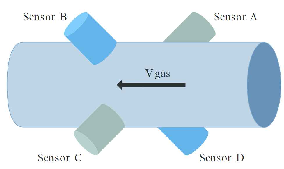
Structure of experimental device of sketch diagram.
As shown in Figure 2, the experimental device consists of an microcontroller unit (MCU) which controls the emission of ultrasonic signal, an ultrasonic sensor driving circuit, a sensor array for transmitting and receiving ultrasonic, a signal receiving circuit with 1 MHz sampling frequency, an field programmable gate array (FPGA) that controls acquisition of ultrasonic signal and a host computer. 1000 groups of ultrasonic signals were recorded by the host computer as the training set for neural network training. Meanwhile, 500 groups of ultrasonic signals are collected as validation set and test set respectively. All data samples are collected with natural gas flow between 0 m3/h and 650 m3/h, and ultrasonic signals at different flow rates are collected as many times as possible. Typical ultrasonic signals in the ultrasonic gas flowmeter system are shown in Figure 3.
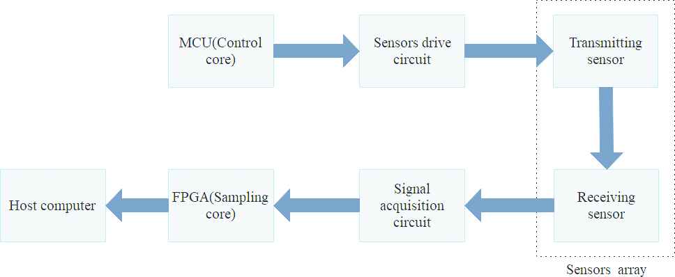
Acquisition process of ultrasonic signal data.
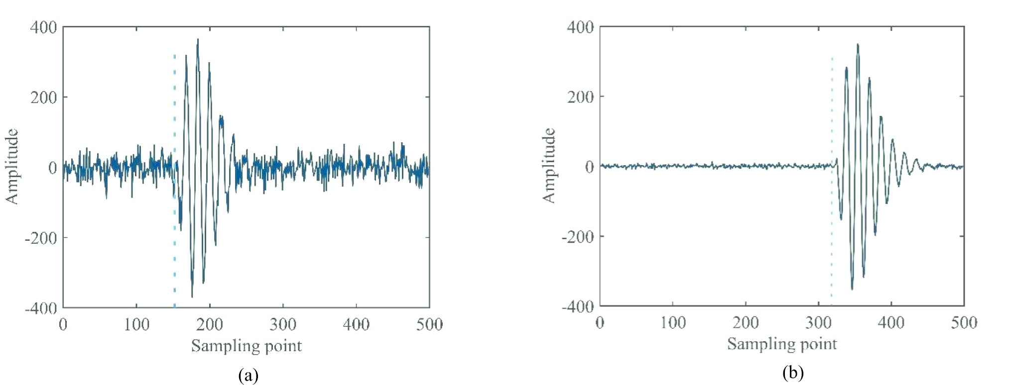
Typical ultrasonic signals in the ultrasonic gas flowmeter system: (a) low signal-to-noise (SNR) and (b) high SNR.
As is shown in Figure 3, the solid lines represent ultrasonic echo signals sampled by sensors, and the dotted lines represent the sampled point corresponding to the arrival time of echo signal. In the training set, the input data is ultrasonic echo signals which is a
2.2. Preprocessing of Ultrasonic Signal
Convolution neural network involves many layers of superposition, and the parameter update of each layer will lead to the change of input data distribution in the upper layer. Through layer upon layer superposition, the change of input distribution in the upper layer will be very dramatic. In order to reduce the influence of distribution changes and speed up model training, it is necessary to normalize the ultrasonic signal.
As is shown in Figure 4(a), the amplitude distribution of sampling point is between −500 and 500 in the actual ultrasonic signal. According to the characteristics of ultrasonic signal, Z-score standardization is utilized to normalize the ultrasonic signal. Z-score is shown as
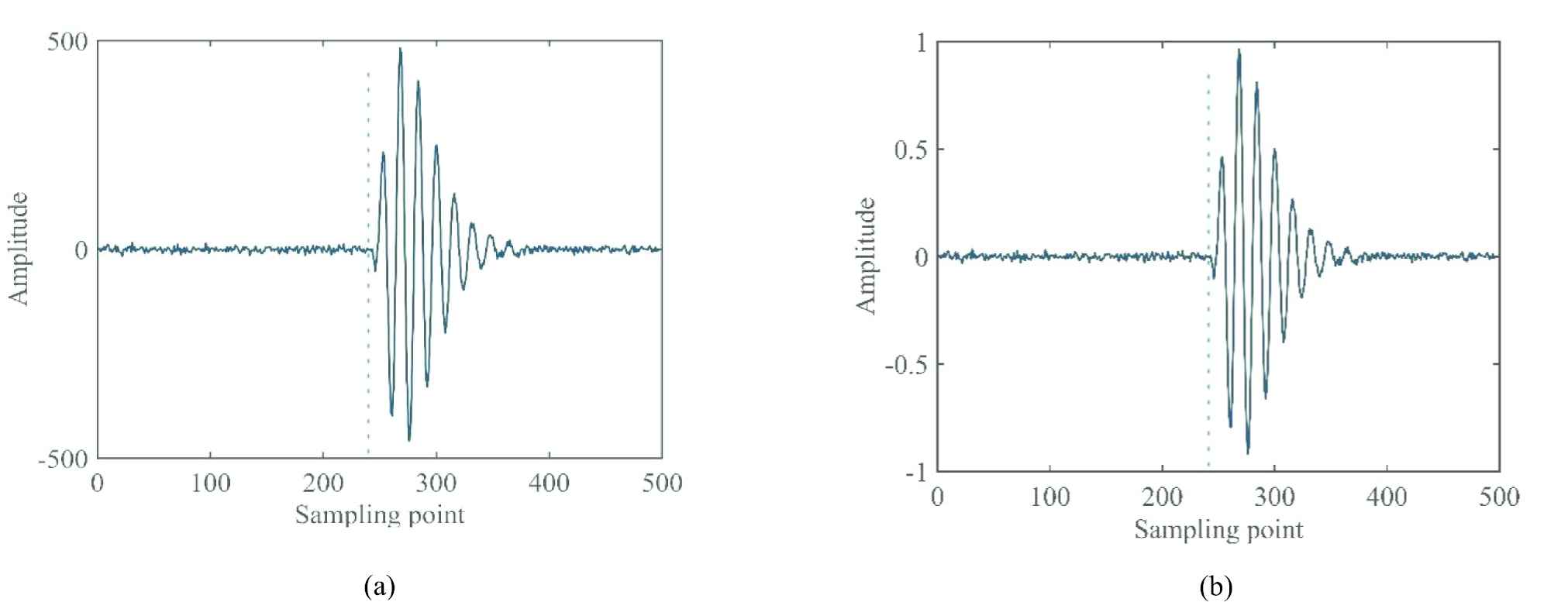
Typical ultrasonic signal in gas flowmeter: (a) original signal and (b) normalized signal.
3. DETECTION OF ARRIVAL TIME BASED ON 1D-CNN
As is mentioned in the introduction early, the core algorithm in the experimental flowmeter is time-difference method, which can be calculated using the following steps. According to the method, the core of the algorithm is to calculate the time difference accurately, which means that it is necessary to determine
3.1. Overview of CNN
CNN is a kind of feedforward neural networks with convolution computation and depth structure, which is one of the representative algorithms of depth learning. CNN has the ability of representation learning and can classify input information according to its hierarchical structure. CNN has been widely used in many visual research fields, such as image classification, face recognition, audio retrieval, ECG analysis, and so on [12,16].
Algorithm 1: Time-difference method
Input:
Velocity of ultrasonic in natural gas, C
Distance between two transducers, L
Time of ultrasonic propagating along gas flow,
Time of ultrasonic propagating against gas flow,
Output:
Velocity of natural gas in pipelines, V
1: calculate the tine difference between
2: calculate the velocity of natural gas by time difference,
Figure 5 shows a 2D CNN model with an input layer that receives a 128 × 128 pixels image. Each convolutional layer after the input layer corresponds to a subsampling layer of the previous layer of neurons that propagates a large number of 2D graphs. In CNN, they are trained (optimized) by the back propagation (BP) algorithm, unlike the manual and fixed 2D filter kernel parameters. However, for the purposes of illustration in Figure 5, kernel size and subsampling factor set to 5 and 2 are the two main parameters of CNN. The input layer is simply a passive layer that accepts the input image and uses its grayscale value channel as a feature map for its three neurons. When propagating forward over a sufficient number of subsampling layers, they are extracted as scalars (1D) at the output of the last subsampling layer. The following layers are the same as the multi-layer perceptron (MLP), fully connected and feedforward networks, which have an output layer that estimates the regression values.
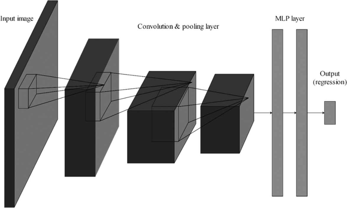
Overview of a sample conventional convolutional neural network (CNN).
In this paper, in order to estimate the arrival time of ultrasonic signal, the structure of typical CNN is modified, including the type of convolution kernel, the setting of layers and the selection of output parameters.
3.2. Arrival Time Detection by 1D-CNN in the Proposed System
As mentioned earlier, 1D-CNN is utilized to estimate the arrival time of ultrasonic signal in the proposed natural gas flowmeter system. The basic structure is shown in Figure 6. As is shown in Figure 6, discrete ultrasonic signals are considered as ID images arranged in chronological order, so the main difference between the traditional 2D-CNN and the proposed 1D-CNN is the usage of 1D arrays instead of 2D matrices for both kernels and feature maps. Accordingly, the original feature extraction of 2D image, such as utilizing 2D convolution matrix and 2D pooling matrix, needs to be replaced by ID signal feature extraction methods, such as ID convolution vector and ID pooling vector. However, the MLP layer is still used in the final output part of the network, which is consistent with the 2D-CNN. Therefore, the proposed 1D-CNN has the same traditional BP formulation.
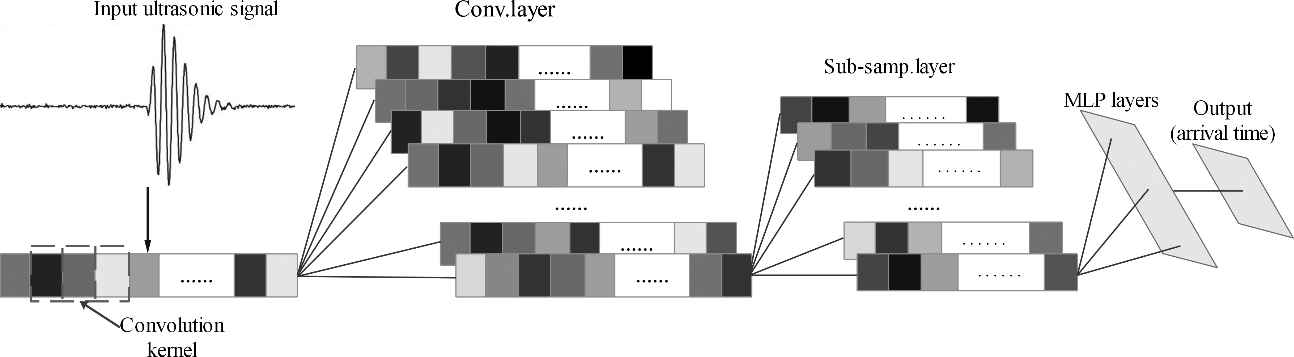
Basic structure of one-dimensional convolutional neural network (1D-CNN) in the proposed system.
In 1D CNN [13], the forward propagation (FP) from a previous convolution layer, m − 1, to the input of a neuron in the current layer, m, can be obtained by
In order to remove redundant information and compress features, downsampling operation is required after the 1D convolution layer, which is achieved by adding a pooling layer. Equation (5) describes the process of downsampling.
In Equation (5),
From the first MLP layer to the last CNN layer, the BP is simply performed as
After doing such a BP calculation, the parameters of the network would be adjusted, which means that a round of iteration is completed.
By repeating the above calculation in the dataset, a trained 1D-CNN can be acquired that the MSE between the predicted ultrasonic signal arrival time by 1D-CNN and the actual arrival time is less than the specified value.
The whole procedure containing the steps of training, validation and testing is based on PyTorch, which is shown in Figure 7.
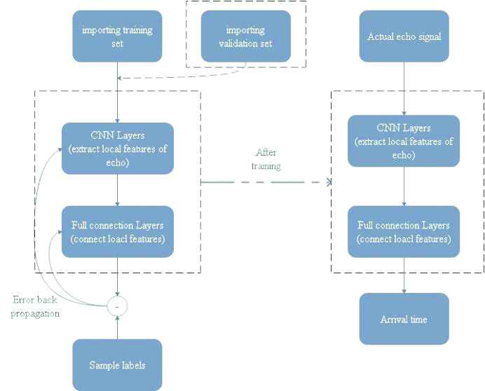
The steps of the whole procedure.
Through a series of experiments referring to adjustment of network parameters, the specific structure of 1D-CNN is determined as shown in Figure 8 finally. The whole network consists of one input layer which receives 1D ultrasonic signal directly, three convolution and pooling layers, one fully connected layer and one output layer that outputs an arrival time of ultrasonic signal. The specific structure of each layer is shown in Table 1. Figure 9 shows the loss function changes in training set and verification set during model training. In order to verify whether the model is overfitted, the confusion matrix of the test set is drawn as is shown in the Figure 10. In the Figure 10, According to the order of sampling time, sampled points are divided into 25 categories, and every category has 20 sampled points. If the sampled point corresponding to the actual arrival time and the predicted sampled point are in the same category, it is considered that the network has estimated the arrival time. The Figure 10 illustrates that the trained network has worked in the testing set. Specific experimental results and analysis will be shown in Section 4.
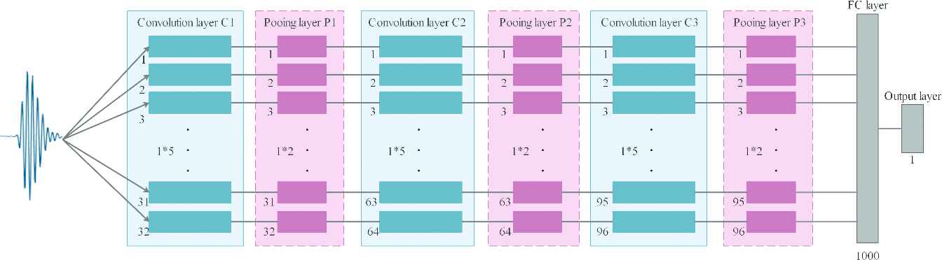
Specific structure of one-dimensional-convolutional neural network (1D-CNN) including one input layer, three convolution and pooling layers, one fully connected layer and one output layer.
| Structure | Parameters |
|---|---|
| Convolution kernel size | |
| Number of convolution kernels | |
| Convolution kernel stride | 1 |
| Pooling size | |
| Pooling stride | 2 |
| Number of neurons in the fully connected layer | 1000 |
1n: represents the nth convolution layer.
Structure parameters of one-dimensional-convolutional neural network (1D-CNN) in the proposed method.
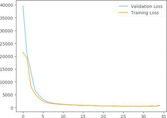
The changes of loss function in the training set and the validation set.
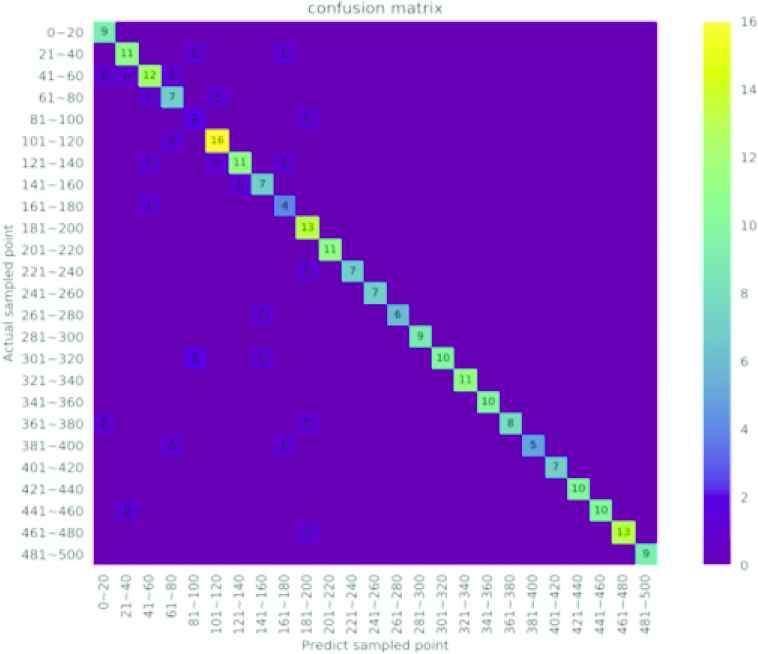
The confusion matrix of model in the testing set.
4. EXPERIMENTS AND RESULTS
As described in Section 3.1, a prototype natural gas ultrasonic flowmeter is built to collect ultrasonic signals, and the hardware platform is also utilized to test the proposed 1D-CNN. In this section, the experimental verification and comparison tests are carried out to verify the effectiveness of the proposed method. Before the experiment, the parameters of 1D-CNN are pretrained by the proposed method in Section 3.2. The training parameters of the experiment are shown in Table 2.
| Experiments | Parameters |
|---|---|
| Operating system | Windows 10 |
| Deep learning framework | PyTorch |
| CPU | AMD R5 2600 |
| GPU | Nvidia RTX 2060 |
| Training method | End-to-end |
| Learning rate | 0.0001 |
| Number of iterations | 50000 |
Training parameters.
4.1. Accuracy of the Proposed Method in Detecting Arrival Time
To test the accuracy of the proposed method, another set of ultrasonic signals with calibrated arrival time is taken as the test set. The test set contains 100 groups of ultrasonic signals collected by the experimental gas flowmeter in different natural gas flows. According to Equations (1) and (2), the arrival time of the ultrasonic signal is obtained from the flow of natural gas, and it is taken as the standard to compare with the arrival time predicted by 1D-CNN. The experimental results are shown in Figure 9 and Table 3. The test results show that the trained 1D-CNN has a high accuracy in the measurement of the arrival time of the ultrasonic wave in the natural gas ultrasonic flowmeter.
| Statistics | Values |
|---|---|
| Mean deviation | |
| Maximum deviation | |
| Root mean-squared error (RMSE) |
Statistics of experimental results.
4.2. Performance Under Different SNRs
To test the stability of the proposed method, the performance of this method is test by comparing with the other method under different signal-to-noises (SNRs). STA/LTA is selected as a comparison method, which is widely used to determine the arrival time of seismic wave, mechanical vibration signal and ultrasonic wave. In this experiment, these two methods are used to measure the arrival time of the same ultrasonic signal collected from the experimental gas ultrasonic flowmeter. And 500 tests were carried out under different SNRs which contain 10 dB, 5 dB and 0 dB by the two methods respectively. Figures 11–13 show the distribution of deviation between measured time
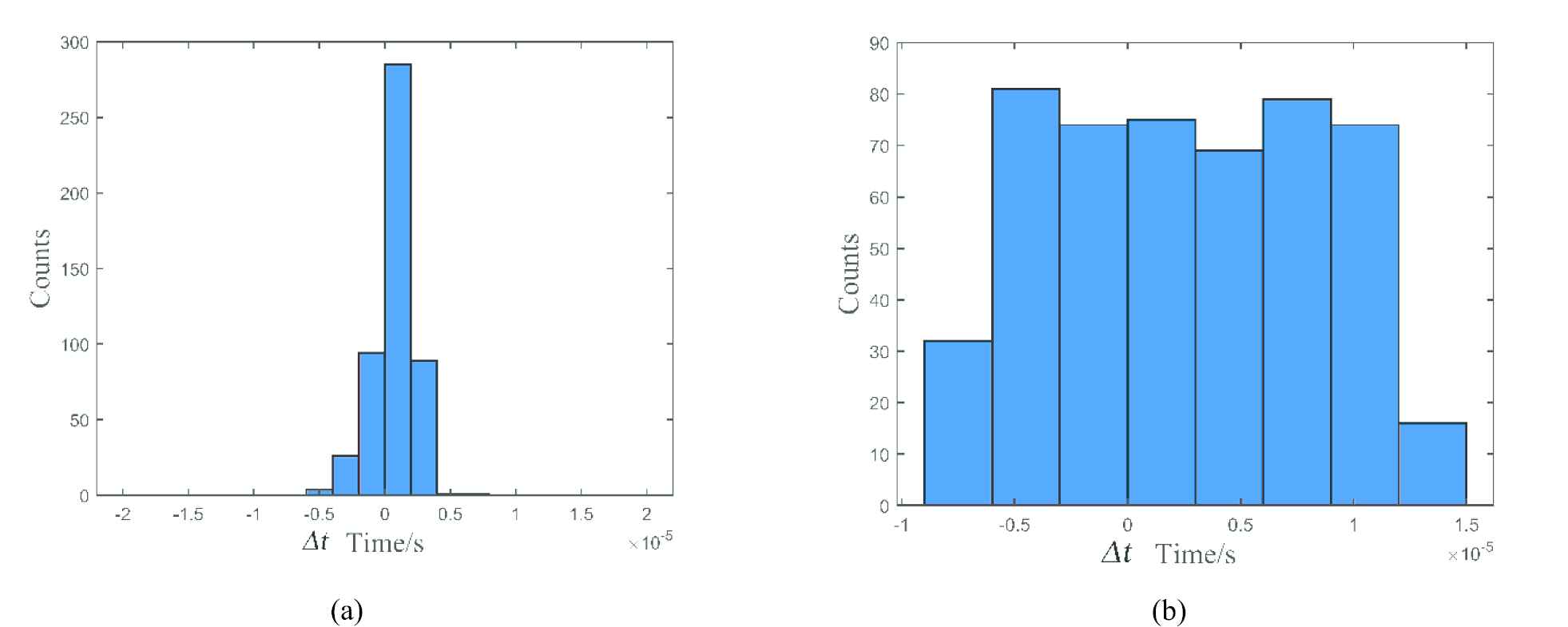
Distribution of deviation in the environment of 10 dB: (a) the proposed method and (b) the short-time average to long-time average (STA/LTA) method.
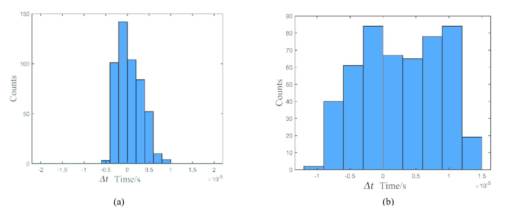
Distribution of deviation in the environment of 5 dB: (a) the proposed method and (b) the short-time average to long-time average (STA/LTA) method.
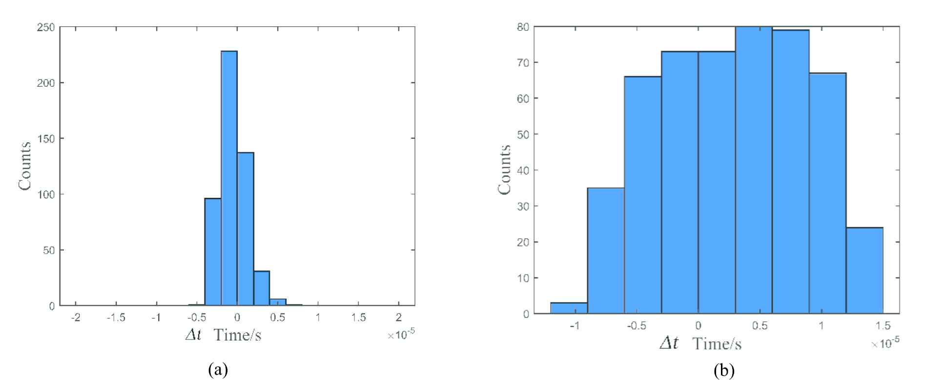
Distribution of deviation in the environment of 0 dB: (a) the proposed method and (b) the short-time average to long-time average (STA/LTA) method.
As is shown in Figures 11–13, most of the deviations distribute close to zero and less than ±5 us using the proposed method, and the distribution is quite intensive. In addition, the distribution shows great stability as the SNR goes down. In contrast, the distributions of
4.3. Discussion of the Experimental Results
Through Figure 14, it can be observed that the deviation between the arrival time of ultrasonic signal predicted by 1D-CNN and the actual arrival time is far beyond the average deviation value in the tests with experiment numbers serial 1 and 2. By observing the original ultrasonic signal corresponding to the experimental serial number, it can be found that in these two groups of tests, the amplitude of the received ultrasonic signal is too small and there is no similar sample in the training set, so the trained 1D-CNN cannot recognize such features, resulting in the final measurement deviation is large. In order to enhance the generalization ability of the proposed method, more experiments will be carried out to collect ultrasonic signals with different characteristics as much as possible. At the same time, a deeper 1D-CNN will be designed to meet the larger training set and improve the generalization ability of the proposed method.
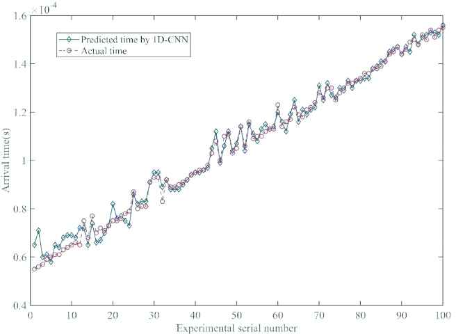
Comparison experiment of deviation between predicted arrival time by one-dimensional-convolutional neural network (1D-CNN) and actual arrival time.
According to Figure 8, Tables 1 and 2, the whole network contains three convolution layers and a full connection layer, the number of convolution kernel in the convolution layers is 36, 64 and 96, respectively. Based on the computing platform shown in Table 2, the average time of a FP process of the proposed method is 75 us. By contrast, the average time of STA/LTA method is 180 us in the same computing platform, which demonstrates that the proposed method has rapid computing performance.
5. CONCLUSIONS
In this paper, a new method is proposed to determine the arrival time of ultrasonic signal which apply to time-difference method that measures natural gas flow in pipeline. The proposed method is different from other methods. It is based on 1D-CNN, which enables it to learn the characteristics of the ultrasonic signal received by the transducer with the proper training and determine the arrival time of the ultrasonic signal. In order to train the proposed 1D-CNN, 1000 sets of ultrasonic signals, collected by transducers as training sets and marked the arrival time, and containing different characteristics such as different arrival time, different SNRs, etc., are prepared.
The proposed method is tested with real ultrasonic signal collected from the experimental gas ultrasonic flowmeter in pipeline. As is shown in Figure 7 and Table 3, the results show that the proposed 1D-CNN has the high accuracy of determining the arrival time of ultrasonic signal. Meanwhile, comparing STA/LTA method, it shows that this method has high anti-noise ability. Further, we consider how to deploy the 1D-CNN to the embedded computing core to measure the arrival time of ultrasound, so as to realize the real-time calculation of natural gas flow in the pipeline.
CONFLICT OF INTEREST
The author declares no conflict of interest.
AUTHORS' CONTRIBUTIONS
The author designs and test the proposed method.
Funding Statement
No funding.
ACKNOWLEDGMENTS
The author wants to acknowledge everyone who has assisted us.
REFERENCES
Cite this article
TY  - JOUR
AU  - Tianjiao Zhang
PY  - 2020
DA  - 2020/08/19
TI  - Flow Measurement of Natural Gas in Pipeline Based on 1D-Convolutional Neural Network
JO  - International Journal of Computational Intelligence Systems
SP  - 1198
EP  - 1206
VL  - 13
IS  - 1
SN  - 1875-6883
UR  - https://doi.org/10.2991/ijcis.d.200803.002
DO  - 10.2991/ijcis.d.200803.002
ID  - Zhang2020
ER  -