
Deep Learning and Higher Degree F-Transforms: Interpretable Kernels Before and After Learning
 , Irina Perfilieva*,
 - DOI
- 10.2991/ijcis.d.200907.001How to use a DOI?
- Keywords
- F-transform; Convolutional neural network; Deep learning; Interpretability
- Abstract
One of the current trends in the deep neural network technology consists in allowing a man–machine interaction and providing an explanation of network design and learning principles. In this direction, an experience with fuzzy systems is of great support. We propose our insight that is based on the particular theory of fuzzy (F)-transforms. Besides a theoretical explanation, we develop a new architecture of a deep neural network where the F-transform convolution kernels are used in the first two layers. Based on a series of experiments, we demonstrate the suitability of the F-transform-based deep neural network in the domain of image processing with the focus on recognition. Moreover, we support our insight by revealing the similarity between the F-transform and first-layer kernels in the most used deep neural networks.
- Copyright
- © 2020 The Authors. Published by Atlantis Press B.V.
- Open Access
- This is an open access article distributed under the CC BY-NC 4.0 license (http://creativecommons.org/licenses/by-nc/4.0/).
1. INTRODUCTION
Deep neural networks (DNNs) significantly improve classification algorithms in various applications, giving a new impact to computer vision, speech recognition, etc. In the proposed contribution, we consider convolution neural networks (CNNs) and the deep learning (DL) methodology for improving parameters of their basic operations.
We are focused on a smart and conscious initialization of convolutional kernels in the first and second CNN layers where neurons have restricted receptive fields. Our motivation stems from the observation that although CNN is able to accurately generate the classification label, it does not report on features that cause this classification. Without an understanding of how DL comes to a solution, there is no guarantee that the trained networks will move from a laboratory to real systems [1]. The reason is that the inputs can significantly change during exploitation, and there is no guarantee that the machine learning tools will work effectively with these changes.
To fill this gap, we propose an insight into why and how CNN makes a decision, or why a specified object has been given a specific classification label. Our approach can be called “preprocessing of methodology” in the sense that we propose a CNN initialization, which ensures that features with known meaning are extracted. Then, we allow the network to learn the initialization parameters so that they can match the available data better.
Our approach differs from many similar ones, based on fuzzy rules, in which the explanation of the CNN decision is based on a posteriori analysis, i.e., after the features are extracted, see [1] and references therein.
We observe that smart preprocessing becomes more and more important in the DL methodology due to the increasing complexity of datasets and objects therein. It heavily depends on a network assignment and consists of traditional de-noising, regularization, reduction of dimensionality, labeling, etc. In most cases, preprocessing is realized in the first convolution layers, together with feature extraction. In subsequent fully connected layers, the extracted features are used for classification, recognition, etc. Therefore, the initial objects are modeled by the extracted features, so that the former ones can be approximately reconstructed from the latter.
Additionally, we observe that similarly to the above, we can characterize the technique of the higher degree fuzzy (F-) transforms [2–4]. This observation leads us to the idea that the higher degree F-transform kernels can be used in the first convolution layers of CNNs that perform recognition or classification.
We are based on long-term work on various approximation models in the theory of fuzzy systems, and in particular, on those, based on the theory of higher degree F-transforms [2–4]. We have collected rich experience regarding creating F-transform-based models in various applications, including image [5–7]/time series [8,9] processing and DL architecture of NNs [10–12].
The principal difference between the DL and the higher degree F-transform is in the criterion of optimality, which is a quality of approximation (F-transform), or a loss function (DL methodology). To reach optimality, it is recommended to refine fuzzy partition and increase the degree of the F-transform [4], or to increase the number of kernels in convolutional layers and increase the number of layers. Both recommendations have the same nature.
The mentioned similarity between the higher degree F-transform and the DL, motivated us to confirm these theoretical considerations by experiments. The latter were conducted in two opposite directions: at first, we trained a neural network with F-transform kernels and estimated its success, and at second, we analyzed kernels of already trained known neural networks and compared them with the F-transform ones. We discussed the obtained results in several conference papers [10–12], where we fully confirmed the hypothesis we made. In the proposed manuscript, we summarize all the results and give extended explanations to the theoretical backgrounds and experimental tests.
The paper is organized as follows: in Section 2, we briefly explain the information-theoretical principles of DNN and the impact of our contribution; in Section 3, we recall essential facts about the higher degree F-transform with the focus on the F
2. DL—A GLIMPSE OF THE THEORY AND POSITION OF OUR CONTRIBUTION TO IT
In this section, we explain the essence of our proposal from a theoretical point of view. We will start with a brief and focused description of DNN, and then explain how we contribute to the current state.
We refer to [13], where the very general characterization of a DNN as a particular computing machine is given: a DNN is a parametric model that performs sequential operations on inputs. Each such operation consists of a linear transformation (e.g., convolution in CNN types), followed by a nonlinear “activation.” An essential factor for DNN success is the availability of large data sets, such as ImageNet and hardware, with a graphics processor, solve to the problem of multidimensional optimization.
In our understanding and approach, we distinguish three key elements in the design of DNN and its corresponding functioning strategy: architecture, the ability to create a good representation of input data, and optimization algorithms. Leaving architecture and optimization aside, we will give a brief description of the second key.
Roughly speaking [13], representation of the input data is any function of it that is useful for the task. If we focus on the most useful (the “best”) representation, then we think of some quantitation, e.g., in terms of complexity or invariance. The relevant line of research is known as representative learning. Despite great interest in this, a comprehensive theory that explains how deep networks with DL methodology contribute to this still does not exist.
However, one thing is clear—the crucial role of the dataset, which is used for training. There is a close connection between the DNN architecture (the number of levels, frames, activations, etc.) and the dataset, which is used to train network parameters. An interesting phenomenon has been reported in [14], where the almost linear relationship was revealed between the sizes of the DNN computational model and the required amount of training data. Obviously, large and multi-object databases require more levels and more complex learning and optimization process.
In a CNN, representation of the input data is realized in the form of a collection of features; the latter are results of convolutions. The collection of features should be complete in the sense of a possible reconstruction (backward representation) of any input object.
Mathematically, the backward “lossy” representation of an object is its approximation. A neural network's ability to produce approximate representations of initial data objects was reported in many papers. However, as shown by earlier work, even neural networks with one hidden layer and sigmoidal activations are universal approximators of functions, see, e.g., [15]. Therefore, the question of why DNNs are advantageous in this regard is still open [13].
One possible explanation is that deeper architectures are better than their shallower counterparts because they are capable of covering not only the requirement of a suitable approximation but also invariance with respect to some rigid transformations. As an example, scattering networks [16] are a class of deep networks whose convolution filter banks are defined by multiple-resolution wavelet families and whose stability and local invariance are confirmed.
This fact supports our initiative in a creation of a “convolutional filter bank” whose kernels are taken from the theory of higher degree F-transforms. Comparing with wavelet kernels, the F-transform ones have clear interpretability in a single and sequential layers in a DNN computation.
It has been proven in many papers [2–4,7] that the higher degree F-transforms are universal approximators of smooth and discrete functions. The approximation on a whole domain is a combination of locally best approximations called F-transform components. They are represented by higher degree polynomials and parametrized by coefficients that correspond to average values of local and nonlocal derivatives of various degrees. If the F-transform is applied to images, then its parameters are used in regularization, edge detection, characterization of patches [7,17], etc. Their computation can be performed by discrete convolutions with kernels that, up to the second degree, are similar to those widely used in image processing, namely Gaussian, Sobel, Laplacian. Thus, we can draw an analogy with the DNN method of computation and call the parameters of the higher degree F-transform features. Moreover, based on a clear understanding of these features’ semantic meaning, we say that a DNN with the F-transform kernels extracts features with a clear interpretation. In addition, the sequential application of F-transform kernels with an up to the second degree gives average (nonlocal) derivatives of higher and higher degrees.
Last but not least, we note that after training DNN, initialized by the F-transform kernels, the shapes of the kernels were not significantly distorted. This fact has been empirically verified on the two datasets: MNIST and CIFAR-10, see Section 4.2 where we compare kernels of various known DNNs after being trained on the same datasets. We observe a similarity of kernel shapes of all considered DNNs. This confirms the stability of the proposed DNN and its sufficiency with respect to the selected datasets.
3. THE F-TRANSFORM OF A HIGHER DEGREE (F m
In this section, we recall the main facts (see [4,18] for more details) about the higher degree F-transform and specifically
3.1. Fuzzy Partition
The F-transform components are the result of a convolution of an object function (image, signal, etc.) and a generating function of what is regarded as a fuzzy partition of a universe.
Definition 1.
Let
for all
The elements of fuzzy partition
In particular, an
Below, we will be working with one particular case of an
A fuzzy partition generated by the triangular-shaped function
3.2. Space L 2 ( A k )
Let us fix
The space
Example 1.
Below, we write the first three orthogonal polynomials
If generating function
We denote
3.3. F m
In this section, we define the
Definition 2. [4]
Let
Explicitly, each
Remark 1.
By the orthogonality of basis polynomials
This fact shows that all subsequent
Definition 3.
Let
The following theorem proved in [4] estimates the quality of approximation by the inverse
Theorem 1.
Let
3.4. F 2
Let us fix
In [4,18], it has been proved that
Without going into technical details, we rewrite (9–11) into the following discrete representations
4. FTNET—CNN WITH F-TRANSFORM KERNELS
In this section, we discuss the details of our neural network design. We chose the LeNet-5 [19] as an architecture prototype and composed a new CNN—FTNet with the kernels initialization taken from the higher degree F-transforms theory [11]. We applied FTNet to several datasets and evaluated the results. For simplicity, we restricted the FTNet architecture to the fixed number of convolutional kernels in the first and second convolutional layers, making the one-to-one correspondence between set of convolutional kernels and set of F-transform kernels
In detail, we replace convolutional kernels in the first and second convolutional layers
The details of the FTNet architecture are given below in Table 1. Note that layer
| Hyper-parameter | Layers | |||||
|---|---|---|---|---|---|---|
| Kernel size | - | - | - | - | ||
| # Kernels | 8 | - | 64 | - | - | - |
| Stride | - | - | ||||
| Pooling size | - | - | - | |||
| # FC units | - | - | - | - | 500 | var |
FTNet architecture.
4.1. Datasets
All the discussed experiments were realized on the following databases: MNIST [20], CIFAR-10 [21], Caltech 101 [16], and Intel Image classification.2 Datasets details are shown in Table 2
| MNIST | CIFAR-10 | Caltech 101 | Intel | |
|---|---|---|---|---|
| Res. | var | |||
| Color | Gray | RGB | RGB | RGB |
| Train | 60k | 50k | 7281 | 14034 |
| Test | 10 k | 10k | 1863 | 3000 |
| Classes | 10 | 10 | 101 | 6 |
Datasets used for experiments.
We convert all datasets to the grayscale because the F-transform kernels extract features with functional meaning and are insensitive to colors. Moreover, we downscale Caltech 1O1 and Intel to
Below, we give a short overview of the known neuro-fuzzy networks, trained on MNIST, and designed for the pattern recognition. We will use MNIST to compare some of the following approaches with FTNet.
Authors of [23] improved the MNIST recognition by optimizing features and architecture, and reached an accuracy of
In [26], the feature selection is based on the wavelet transform that uses 2D scaling moments and various classifiers (support vector machines/classifiers, artificial neural networks, neuro-fuzzy classifiers, and others). The SVM classifier demonstrates the best accuracy of
Similar to MNIST, the database of handwritten characters Chars74k [27] has been studied in [28]. The authors used a three-fold cross-validation and achieved
In the recent publication [29], the Fuzzy Deep Belief Net (FDBN) was proposed to classify MNIST with different types and levels of noise. The FDBN architecture is described in [30,31], where the authors declared better results than using the standard Deep Belief Networks.
4.2. Performance of FTNet and Comparison with the He Initialization
In this section, we compare FTNet initialized with F-transform kernels with Baseline network using the same architecture and He initialization [32]—one of the most common initializations.
We follow He initialization and scale F-transform kernels to
We remark that in the FTNet, the
Figure 1 shows normalized results of training Baseline network and two variants of FTNet. FTNet (red graph curve) corresponds to F-transform kernel initialization, where kernels are allowed to learn. During the learning the kernels are modified to a certain degree. From the graphs, we can see that F-transform kernels initialization is advantageous over He initialization. The Second variation does not allow F-transform kernels to learn and kept unchanged. We can observe that while it has lower loss values at the beginning of training, it falls behind later on. The advantage of static FTNet is higher training speed and lower number of trainable parameters; this can be particularly beneficial to overfitting problem and problem of small datasets. Lastly, static FTNet kernels and features they extract are clearly interpretable.
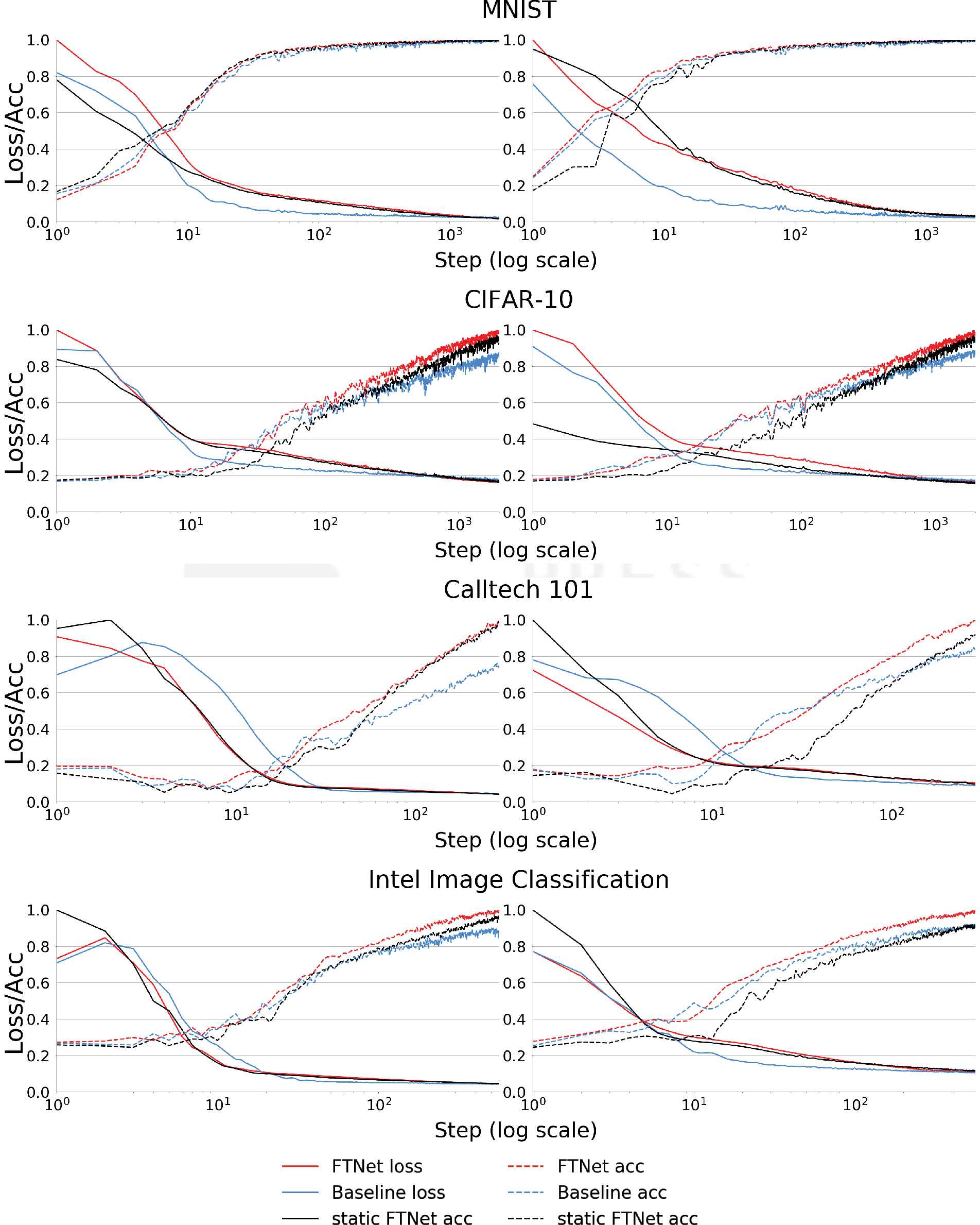
Results of 2 epoch training on datasets. In the left column are results of training with FTNet C1 initialized with F-transform kernels. Second column contains results of training with both C1 and C3 initialized with F-transform kernels. Note that both accuracy and loss are scaled to [0, 1].
We trained each network 10 times in 2 epochs. For the training, we used Adam (
Since disabling trainability of
| Dataset | FTNet |
Baseline | |
|---|---|---|---|
| Trainable | Nontrainable | ||
| MNIST | 320s | 299s | 315s |
| CIFAR-10 | 290s | 252s | 289s |
| Caltech 101 | 20s | 15s | 20s |
| Intel | 65s | 53s | 66s |
Average training times for FTNet and its variants and baseline network.
Due to MNIST being the most common dataset, we use it to compare FTNet with other approaches. In Table 4 you can see comparison of FTNet and results reported in selected publications (the latter are indicated by their reference numbers in the first row).
| [26] | [29] | [23] | [33] | [34] | FTNet |
|---|---|---|---|---|---|
Comparison of FTNet with other approaches on MNIST.
| None | Trainable | F-transform kernels | |
| Max-pool | Nontrainable | Kernels |
|
| Stride | - | - | |
| VACL | - | - | - |
The four hyperparameters values:
4.3. F-Transform Kernels as Preprocessing
One can use the F-transform to process data before feeding them into a network. We perform a comparative experiment between the F-transform and recently published fuzzy preprocessing technique—IRFF [35]. IRFF processes images in a convolutional manner, saving minimum, maximum, and central pixel values from a selected neighborhood. In general, the IRFF preprocessing increases the accuracy of a network.
We conducted experiment, comparing the IRFF and F-transform performances on CIFAR-10 using ResNet34 [36] with Shake-Shake regularization [37]4 that achieved accuracy up to
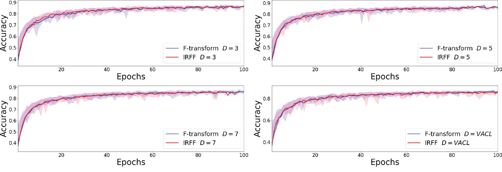
Average accuracy (over 10 runs) of ResNet34 with Shake-Shake regularization on CIFAR-10 over 100 epochs. Network uses Adam(α = 1e − 3), cross entropy loss, early stopping, batch size 128, and light augmentation (width/height shift up to 0.1 and vertical flipping).
5. FTNET HYPERPARAMETERS AND INTERPRETABILITY
To assure that we use a proper combination of hyperparameters, we searched through the hyperparameters space, determined by four hyperparameters: Initialization
Let us describe the functionality of the hyperparameters mentioned above:
Scale-space [41] inspired VAriable Convolutional Layer (VACL) value of
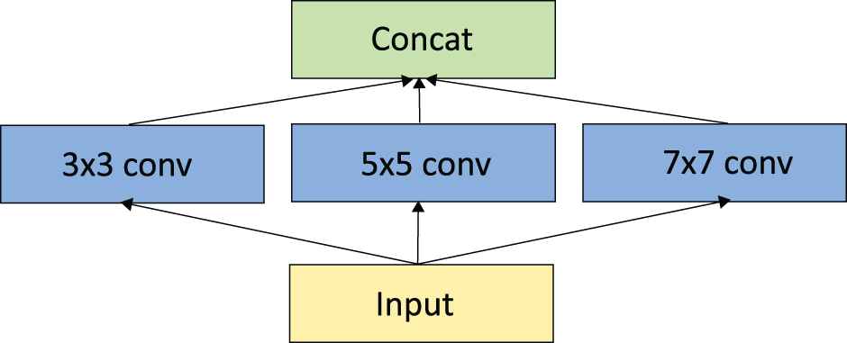
Scheme of the convolutional layer with variable kernels sizes, realized as multiple convolution layers with their outputs concatenated.
Using VACL in
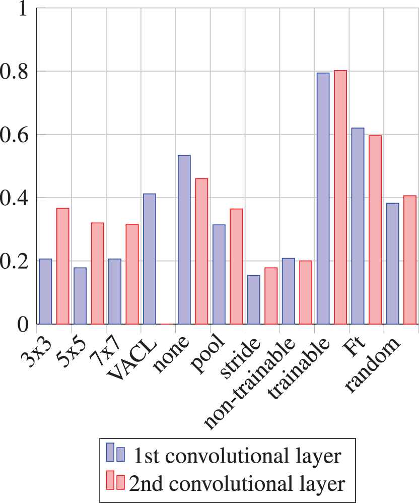
Relative frequencies of the hyperparameters values for C1 and C3 within the first 500 best combinations in terms of accuracy after 3 epochs of learning on MNIST.
An unexpected result is a high relative frequency of the ”no subsampling” in both cases while stride being worst out of the three.
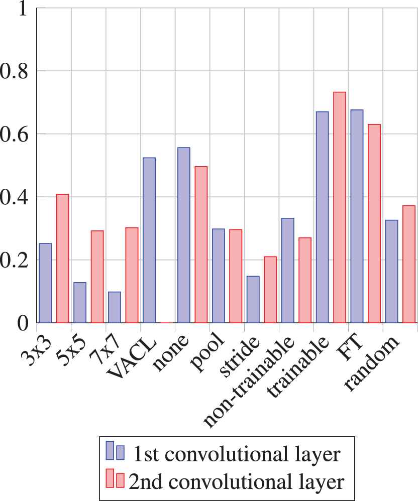
Relative frequencies of the hyperparameters values for C1 and C3 within the first 500 best combinations in terms of accuracy after 3 epochs of learning on CIFAR-10.
As an additional argument in favor of our technique, we visualize the F-transform kernels in Visualization of the eight F-transform kernels before and after training (100 epochs) in C1. The first two rows contain 3 × 3 kernels (training does not change the kernels significantly). The second two rows contain 5 × 5 kernels (the training added some variational details) and the third two rows contain 7 × 7 kernels (the training changed the F0-transform kernels transforming them to the rotated F1-fransform).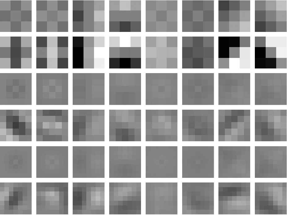
Up to the small contrast changes,
The shapes of
The shapes of
Thus, we can summarize achieved results:
The scale-space inspired VACL is the most frequent size of the convolution kernels in the first convolutional layer of the considered CNN, trained on both datasets.
The initialization of
Excluding subsampling from CNN's architecture increases network accuracy; however, it contributes to an undesirable effect of overfitting.
Including subsampling into CNN's architecture leads to a quicker decrease of a loss function.
The F-transform kernels in the first layer
5.1. Semantic Meaning of Principal Kernels in Convolutional Layers
In this subsection, we tackle the problem of interpretability from the opposite angle. Instead of initializing a network with predefined kernels, we examine the first convolutional layers and the corresponding to them (already trained) kernels taken from several well-known networks. The purpose is to find general semantic meanings of kernels and through them compare with the F-transform kernels.
We tried to assign interpretation to kernels of already trained CNNs: We based on the known interpretation of the higher degree F-transform kernels and wished to reveal the similar meaning of kernels extracted from the first convolutional layer of several frequently used CNNs, trained on the ImageNet [43]. Let us review some of the existing contributions that connect both DL and fuzzy disciplines.
We selected 6 networks: VGG16 [44], VGG19 [44], InceptionV3 [45], MobileNet [46], ResNet [36], and AlexNet [47] as the representative examples of CNNs. All of the networks were trained on ImageNet [43], using the same training database, consisting of
We extracted kernels from the first convolutional layer of all considered networks and analyzed whether there are similarities among kernels across the networks. To reduce the space of kernels, we first apply the hierarchical clustering on every network kernel set separately, and then, look for the similarities among clusters. The medoids of the found clusters are shown in Figure 7.
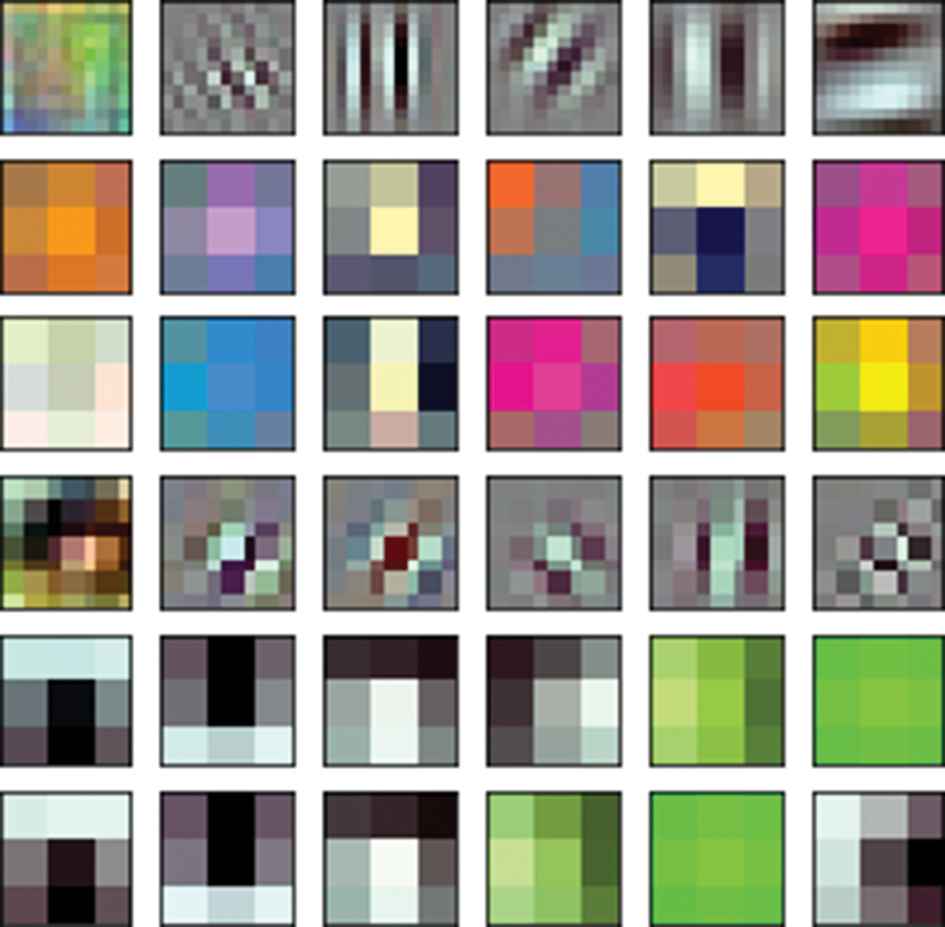
From top to down: the medoids of the clusterized kernels from the first convolutional layer of AlexNet, InceptionV3, MobileNet, ResNet, VGG 16, and VGG 19.
We observed that the extracted clusters contain similar elements (kernels) across the different networks that share one of the following characteristics/functionality: gaussian-like; edge detection (with various angle specifications); texture detection; color blobs.
If we compare the semantic meaning of the extracted clusters (in terms of the above-given characteristics/functionality) with that of the F-transform kernels in the FTNet, then we see the coincidence in the first two items from the above-given list. To be more precise, the F
The above-formulated general conclusion relates to the disclosed semantic meaning of convolutional kernels. This knowledge is helpful for the optimal and nonexhaustive design of CNNs.
6. CONCLUSION AND THE FUTURE WORK
We have proposed a new CNN learning methodology that is focused on a smart preprocessing with the meaningful initialization of CNN kernels in the first two layers. The methodology is based on the fuzzy modeling technique—F-transform. As a result, we have designed a new CNN-type network called FTNet.
The performance of FTNet was examined on several datasets and on them it converges faster in terms of accuracy/loss than the baseline network, subject to the same number of steps.
We compared the F-transform kernels in the first layer before and after training. We observed that the kernels remain unchanged. Moreover, their shapes are similar to the shapes of extracted kernel groups from the most known CNNs.
All these facts confirm our hypothesis that the smart initialization of the first layers kernels can be proposed based on their semantic meaning and the general network designation.
Our future work will be focused on neural nets with larger number of layers and other than recognition objectives.
CONFLICTS OF INTEREST
The authors declare no conflict of interest.
AUTHORS' CONTRIBUTIONS
Authors Irina Perfilieva and Vojtech Molek made equal contributions.
ACKNOWLEDGMENTS
The work is supported by ERDF/ESF “Center for the development of Artificial Intelligence Methods for the Automotive Industry of the region” (No. CZ.02.1.01/0.0/0.0/17_049/0008414).
Footnotes
The text of this and the following subsection is a free version of a certain part of [4] where the theory of a higher degree F-transform was introduced.
α - learning rate, γ - decay, λ - strength of regularization.
Subsampling operation originates from Hubel and Wiesel [38]; comparison of pooling can be found in Ref. [39].
We have employed dropout to reduce network overfitting.
ImageNet database content depends on the year of ILSVRC competition.
REFERENCES
Cite this article
TY  - JOUR
AU  - Vojtech Molek
AU  - Irina Perfilieva
PY  - 2020
DA  - 2020/09/16
TI  - Deep Learning and Higher Degree F-Transforms: Interpretable Kernels Before and After Learning
JO  - International Journal of Computational Intelligence Systems
SP  - 1404
EP  - 1414
VL  - 13
IS  - 1
SN  - 1875-6883
UR  - https://doi.org/10.2991/ijcis.d.200907.001
DO  - 10.2991/ijcis.d.200907.001
ID  - Molek2020
ER  -