
Woodland Labeling in Chenzhou, China, via Deep Learning Approach
 , Yujing Yang1, Ji Li1, Yongle Hu2, Yanhong Luo3, *, Xin Wang1, *
- DOI
- 10.2991/ijcis.d.200910.001How to use a DOI?
- Keywords
- Woodland labeling; Convolutional network; Deep learning; Dense fully convolutional network (DFCN)
- Abstract
In order to complete the task of the woodland census in Chenzhou, China, this paper carries out a remote sensing survey on the terrain of this area to produce a data set, and used deep learning methods to label the woodland. There are two main improvements in our paper: Firstly, this paper comparatively analyzes the semantic segmentation effects of different deep learning models on remote sensing image datasets in Chenzhou. Secondly, this paper proposed a dense fully convolutional network (DFCN) which combines dense network with FCN model and achieves good semantic segmentation effect. DFCN method is used to label the woodland in Gaofen-2 (GF-2) remote sensing images in Chenzhou. Under the same experimental conditions, the labeling results are compared with the original FCN, SegNet, dilated convolutional network, and so on. In these experiments, the global pixel accuracy of DFCN is 91.5%, and the prediction accuracy of the “woodland” class is 93%, both of them perform better than that of the other methods. In other indicators, our method also has better performance. Using the method of this paper, we have completed the land feature labeling of Chenzhou area and provided it to customers.
- Copyright
- © 2020 The Authors. Published by Atlantis Press B.V.
- Open Access
- This is an open access article distributed under the CC BY-NC 4.0 license (http://creativecommons.org/licenses/by-nc/4.0/).
1. INTRODUCTION
Woodland plays an important role in promoting ecological construction, improving ecological environment, ensuring human health, and maintaining social sustainable development. Therefore, how to label the woodland accurately is worth studying.
In recent years, with the development of deep learning, convolutional neural networks have performed quite well in computer vision recognition tasks, such as image classification [1,2], targets detection [3,4], and semantic segmentation [5]. For example, Krizhevsky et al. [1] used AlexNet of approximately 60 million parameters with 5 convolutional layers and 3 fully connected layers to win the 2012 champion of ImageNet Large-scale Visual Recognition Challenge [6]. In addition, VGG [7], GoogleNet [8], and ResNet [9] have also achieved great success. Sun et al. investigate quantized synchronization control problem of memristive neural networks (MNNs) with time-varying delays via super-twisting algorithm [10]. Wang et al. investigated the synchronization of multiple memristive neural networks (MMNNs) under cyber-physical attacks through distributed event-triggered control [11]. Yu et al. [12] designed a 5D hyperchaotic system to coexist multiple attractors, and used the system to generate random numbers for image encryption. Huang et al. designed the shape synchronization and image encryption of 4D chaotic system [13]. Wang et al. [14] designed SSF-Net to solve the feature extraction problem of sparse data, and IVGG Models [15] improved network performance. Based on these studies, we further improved the network for remote sensing image semantic segmentation.
With the application of deep learning, it is of great significance to extract information in remote sensing images using deep neural networks. DenseNet is a deep network architecture which has performed well in image classification in recent years. By using dense connections, the problem of feature map information disappearance caused by the increase of network layer is effectively alleviated, and the deep network converges more easily in training [16]. In this work, we improved the feature extraction module of FCN by replacing the original VGG-16 with DenseNet, optimized the skip architectures, and proposed a new dense fully convolutional network (DFCN).
Furthermore, this paper provided a new dataset showing the remote sensing woodland of Chenzhou, China. The remote sensing images, which come from GF-2 satellite with spatial resolution of 0.8 meters, show all kinds of spatial information of farmland, woodland, river, wasteland, buildings, and so on. The data set is the first completed data set of forestry resources in Chenzhou based on GF-2 satellite images. At the same time, the dataset can provide relevant samples for the classification of woodland in the same landscape environment.
In addition, we also analyze the performance of ResNet [9] and some other semantic segmentation models, such as SegNet [17] and dilated convolutional network [18] on the same data set.
By using DFCN, woodland and other areas in GF-2 satellite images of Chenzhou are labeled, and the results are provided to relevant forestry departments. By using the labeling results, relevant personnel can further analyze the changes of the woodland area and ecology in this region, so as to take corresponding measures to protect the forestry resources and develop the forestry economy. At present, based on GF-2 remote sensing images, we regularly provide labeling image data products to the land resources and forestry departments of Chenzhou.
2. RELATED WORK
Image semantic segmentation is an important method in the field of computer vision. Before applying the deep learning model to semantic segmentation, Shotten et al. [19] proposed semantic texton forests for image categorization and segmentation. After AlexNet [1] won the ImageNet image classification competition in 2012, the potential and performance of convolutional neural networks have attracted more and more attention. In 2015, Long et al. [5] proposed a fully convolutional network for image semantic segmentation. The proposed model creatively realized the leap from image classification field to pixel level classification of deep convolutional neural network. After that, fully convolutional network (FCN) has been used in image semantics segmentation research for a long time. For example, Unet [20] was based on FCN, which achieved good results in semantic segmentation of biomedical images. DeepLab [21] used a deconvolution operation for up-sampling. Based on Encoder-Decoder, Badrinarayanan et al. [17] proposed the SegNet architecture, in which the position information discarded in the pool layer was utilized in the process of up-sampling so as to greatly reduce the network parameters. Fully convolutional DenseNets [22] applied dense blocks in the semantic segmentation model in order to enhance feature extraction and feature reuse. Chen et al. [23] designed modules which employ atrous convolution in cascade or in parallel to capture multi-scale context by adopting multiple atrous rates. Considering that semantic segmentation requires rich spatial information and a large acceptance domain, BiSeNet [24] designed two parts, Spatial Path and Context Path, and tried to use a new method to keep both Spatial Context and Spatial Detail at the same time. Fu et al. [25] addressed the scene segmentation task by capturing rich contextual dependencies based on the self-attention mechanism. Liu et al. [26] investigated the knowledge distillation strategy for training small semantic segmentation networks by making use of large networks. There is also a lightweight network for image segmentation and classification [27]. In addition, the semantic segmentation also has similarities with image super-resolution reconstruction [28].
Semantic segmentation also plays an important role in remote sensing image research. Mitra et al. [29] and Bilgin et al. [30] both used support vector machines (SVMs) to segment remote sensing images. Marmanis et al. [31] improved semantic image segmentation with boundary detection, which achieved good results on ISPRS 2D semantic annotation data set. Cheng et al. [32] proposed a simple but effective method to learn discriminative CNNs (D-CNNs) to boost the performance of remote sensing image scene classification. Hamida et al. [33] presented recent Deep Learning approaches for fine or coarse land cover semantic segmentation estimation. Wang et al. [34] used deep feature-based adaptive joint sparse representation in image object recognition.
3. DENSE FULLY CONVOLUTIONAL NETWORK
In this section, we first introduce the relevant principles of FCN, and then introduce the DFCN method proposed in this paper. At the end of this section, we introduce the evaluation criteria.
3.1. FCN
FCN is mainly composed of feature extraction module (downsampling module), skip architectures, and up-sampling module, as shown in Figure 1.
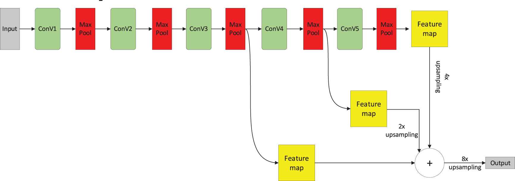
Structure of fully convolutional network.
If the size of the input image is x × y, after 3 pooling operations, the image size changes to (x × y)/8. Similarly, after 4 and 5 pooling operations, the image sizes are (x × y)/16 and (x × y)/32. In order to make full use of the characters both in deep layers and shallow layers, FCN put forward the skip architectures. In FCN, the feature maps generated after 5 times pooling operations are 4 times upsampled. Then another group of feature map generated after 4 times pooling operations are double-sampled. Next, the feature maps of the two groups obtained above are concatenated with the feature map obtained after 3 times pooling operations. Finally, 8 times up-sampling is used to restore the resolution of the original image.
3.2. DFCN
Because the dense connection form of DenseNet can reuse the feature maps effectively and alleviate the problem of information disappearance of the feature maps due to the deepening of network, the DenseNet is used to replace VGG-16 in FCN model for feature extraction. On this basis, we further adjust the skip architectures and propose DFCN model, as shown in Figure 2.

Schematic diagram of dense fully convolutional network (DFCN).
DenseNet is mainly composed of dense blocks and transition layers, as shown in Figure 3. For ordinary convolution block, the output of layer

Schematic diagram of dense block.
In DenseNet, the input of layer
It can be seen from Formula (2) that the input of the
In addition, the transition layer in Figure 2 mainly performs a dimensionality reduction operation on the feature map generated by the dense block. Its main components are shown in Figure 4.
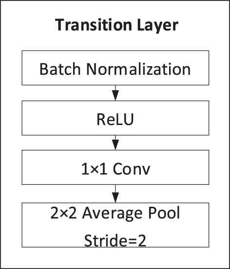
Schematic diagram of transition layer.
In transition layer, the input feature maps are first regularized through the batch normalization (BN) and then activated through the rectified linear unit (ReLU) activation function. Since feature maps generated by dense blocks are often increased, in order to avoid the training difficulties caused by too many feature maps, the input feature maps are convoluted by 1 × 1 convolution kernels. This operation is equivalent to reducing the dimension of feature size while keeping the original image size unchanged. Then an average pooling layer is used after 1 × 1 convolution layer. Therefore, the transition layer effectively reduces the parameters in network training.
Similar to the structure of DenseNet, DFCN also uses 4 dense blocks, so we can initialize and fine-tune the DFCN model by using the parameters pre-trained by ImageNet. We also use a new skip connection in DFCN. In the skip connection of FCN, after have pooled for 5 times, the feature maps are taken 4 times up-sampling. After have pooled for 4 times, the feature maps are taken 2 times up-sampling. Then the two results are combined with the feature maps that have been pooled for 3 times. Finally, the whole feature maps are taken 8 times up-sampling.
Different from FCN, in the skip connection of DFCN, the feature maps are taken 2 times up-sampling after have pooled for 5 times and combined directly with the feature maps after have pooled for 4 times. Then the above results are taken 2 times up-sampling and combined directly with the feature maps after have pooled for 3 times. Finally, the whole feature maps are taken 8 times up-sampling. In our skip connection, the transposed convolution [32] operation is used in up-sampling, as shown in Figure 2.
4. DATA SETS AND EXPERIMENT SETUP
4.1. Data Set
We collected remote sensing image data of Chenzhou, Hunan, China, with GF-2 satellite, and constructed a forest land classification data set. The spatial resolution of GF-2 satellite is 0.8 m. We named the data set GF2-CZ data. The reason for choosing Chenzhou for remote sensing data is that Chenzhou has typical southern China landform and a large proportion of forestry area. Therefore, the establishment of woodlands classification data set in Chenzhou can provide a standard database for the study of woodlands labeling methods of similar terrains in south China. According to the administrative division of Chenzhou, we divided the remote sensing image into six regions and get six original high-resolution remote sensing images. The corresponding names, area sizes, image sizes, longitude, and latitude information of the image center of the six towns are shown in Table 1. Figure 5 shows the original remote sensing image of Wulipai town in Chenzhou.
| Town | Area (km2) | Image Size | Center Latitude and Longitude |
|---|---|---|---|
| Wulipai town | 5.02 | 3000*2100 | |
| Taiping town | 3.12 | 2300*1700 | |
| Xiangyindu town | 2.82 | 2200*1600 | |
| Youshi town | 5.71 | 3400*2100 | |
| Gangjiao town | 4.72 | 2800*2100 | |
| Liaowanpin town | 4.89 | 2900*2100 |
Detailed information of remote sensing images.
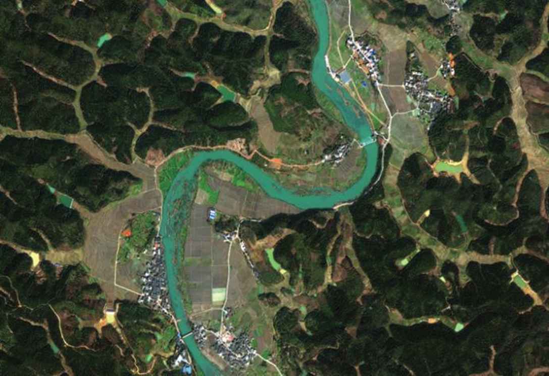
High-resolution remote sensing image of Wulipai town.
After obtaining 6 original images, we used the remote sensing image processing platform ENVI (the Environment for Visualization Images, http://www.enviidl.com/) to respectively carry out quick atmospheric correction (QUAC). The main purpose was to eliminate the influence of atmosphere and illumination on the reflection of ground objects. Here we mainly used it to expand the original data and obtain 6 pairs of remote sensing images.
According to the training requirements, the data were marked manually. In order to minimize labeling errors, labeling work was carried out under the guidance of relevant technical personnel of Hunan provincial forestry department. The data were divided into 7 classes (numbered class 0–6, respectively), which were farmland (background), woodland, bare land (wasteland), water, buildings, roads, and furrows. Among them, bare land (wasteland) and furrow were also labeled as the areas we were interested in, because bare land and wasteland were areas that need to be harnessed. They were of great significance to statistics of the proportion of forest land area and to help relevant departments formulate forestry policies. Furrows were typical landforms in southern China, so they were also labeled as an independent class. Finally, the labeled ground truth maps were 16-digit PNG images. Figure 6 shows a visualization of the ground truth map of Wulipai Town.
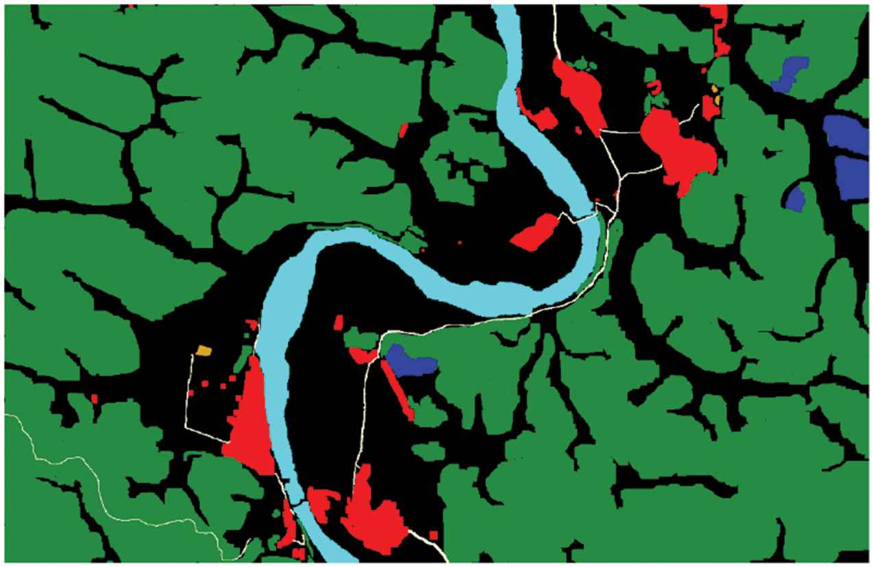
The ground truth of Wulipai town, Chenzhou. The ground truth map is divided into 7 classes: 0 for background(black), 1 for woodland(green), 2 for bare land or wasteland(dark blue), 3 for waters(light blue), 4 for buildings(red), 5 for roads(white), and 6 for furrows(orange).
Data expansion and data augmentation were also carried out for the above 6 pairs of original images. The main processing methods were random window sampling with window of 256 × 256 size, random gamma transform, rotation 90 degrees, 180 degrees, 270 degrees, blur, add salt noise, left and right flip, up and down flip, and so on. After data expansion, we made a GF2-CZ data set for deep learning. The training set in the experiment included the images except the Liaowanpin town images. It contained 10,000 remote sensing images, each with a size of 256 × 256. The test set was obtained by data enhancement and expansion of remote sensing images in Liaowanpin town. It contained 2000 remote sensing images, each of which has a size of 256 × 256. Therefore, the test images in our experiment were completely untrained remote sensing images. Figure 7 shows a visualization of some samples and corresponding tags in the test set.
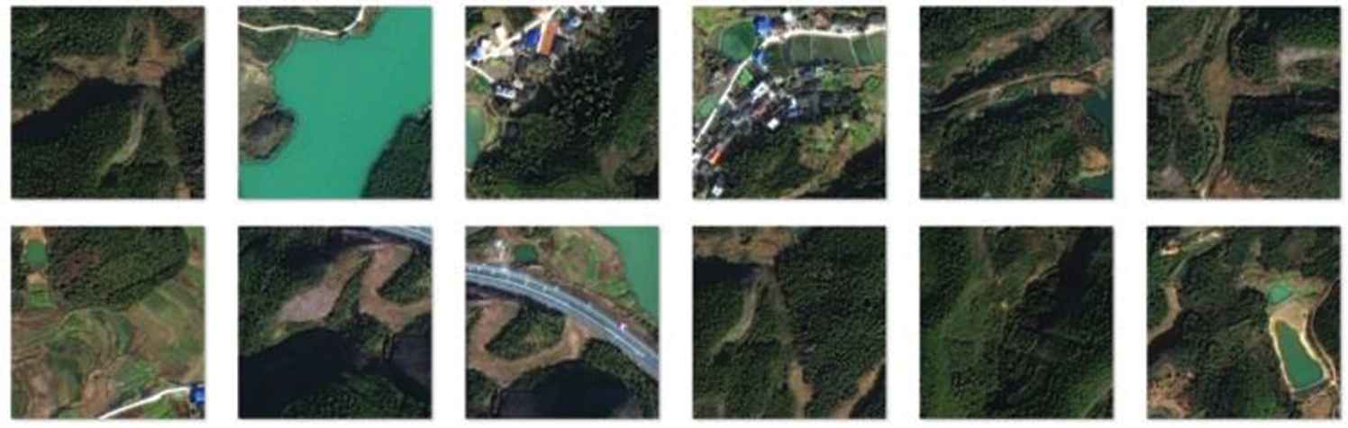
Examples in training set.
4.2. Experimental Platform
Our experiments were carried out under the same platform and environment to ensure the credibility of comparisons between different network models. The specific software and hardware configuration information are shown in Table 2.
4.3. Evaluation Criteria
Based on the evaluation criteria adopted in most semantic segmentation model, the pixel accuracy (PA), mean intersection over union (MIoU), and frequency weighted intersection over union (FWIU) were used to demonstrate the effectiveness of the proposed method [1].
| Configuration | Configuration Parameter |
|---|---|
| Operating system | Windows 10 |
| CPU | Intel i7 3.30GHz |
| GPU | GTX1080Ti(11G) |
| RAM | 16G/DDR3/2.10GHz |
| cuDNN | CuDNN 10.0 |
| CUDA | CUDA10.0 |
| Frame | PyTorch |
| IDE | Pycharm |
| Programming language | Python |
Experimental environment configuration.
If the image pixels can be divided into
For single class labeling, in order to evaluate the effect, we mainly adopted the precision, recall rate, and
4.4. Architecture and Training Details
Parameters of DenseNet network after ImageNet pretraining [35] were used to initialize parameters of feature extraction module of DFCN. In up-sampling process, bilinear interpolation was used to initialize the parameters of the transposed convolution, and the negative log likelihood loss (NLLLoss) function was selected as the loss function. The NLLLoss function is useful to train a classification problem with C classes and it is mainly used for the semantic segmentation of multi-class prediction in Pytorch. In the training stage, Batchsize was set to 4, SGD with the momentum was used as the optimization function, momentum was set as 0.9, and the learning rate was set to 0.01, which decreased to 0.001 after 50 epoches.
We regularized the model with a weight decay of 0.0001. After each epoch, we calculated the loss function, global PA, and MIoU of the training set and test set, respectively. The specific configuration information of the model Dense121-FCN (DFCN121, in which the pretraining model was DenseNet121) with the best performance in our experiments is shown in Figure 8. As shown in Figure 8, in order to initialized the network parameters using the pretraining model, the parameter settings of feature extraction part of our network were basically the same as those of DenseNet121 [6]. The up-sampling module was mainly realized by transposed convolution. When up-sampling times was 2, the convolution kernel size was set to 4 × 4, the step size was 2, and padding = 1. For 8 times up-sampling, the convolution kernel size was 16 × 16, the step size was 8, and padding = 4.
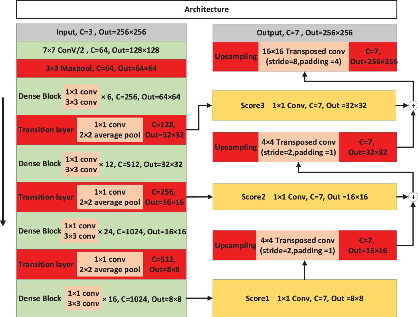
Schematic diagram of dense fully convolutional network (DFCN121) configuration.
The pseudo code of the training and labeling process is shown in Table 3.
| Algorithm 1 Training and Labeling Process |
|---|
|
Input: remote sensing images of ChenZhou Output: trained DFCN models 1: Divide GF2-CZ dataset into training set and test set. 2: Apply data augmentation on training set. 3: Train DFCN and generate trained models: Initialisation: pretrained DenseNet model 4: for i = 1 to N do 5: Train(DFCN, train_img, img_label, class_weight) 6: if (i == l1) then 7: save(DFCN models) 8: end if 9: end for 10: return trained DFCN models |
The pseudo code of the training and labeling process.
5. EXPERIMENTAL RESULTS COMPARISON AND ANALYSIS
In the experiments, we adopted two types of DFCN models, DFCN121(DFCN121-A, DFCN121-B, DFCN121-C) and DFCN169, and compared them with the original FCN [5], SegNet [17], Res-FCN [9], dilated convolutional network [18], and Unet [20] on the same data set of high-resolution remote sensing image. In our comparison experiments, considering the convergence of network training, we used the same dilated convolutional network as Ref. [18], but did not use its multi-scale context aggregation architecture, because the use of multi-scale context aggregation architecture will cause the network training to fail to converge without pre-trained.
We mainly analyzed the experimental results in 4 aspects: the performance of various models, the stability and convergence speed of model training, the woodland labeling effect, and the visualization of woodland label results.
| Model | Parameters (M) | MIoU (%) | FWIU (%) | Pixel Accuracy (%) | Training Time per Image (ms) | Test Time per Image (ms) |
|---|---|---|---|---|---|---|
| FCN-8s [5] | 14.7 | 51.16 | 84.61 | 90.55 | 23.7 | 11.5 |
| FCN-32s [5] | – | 52.22 | 84.28 | 90.35 | 24 | 11 |
| FCN-8s(our) | 14.7 | 51.78 | 85.40 | 91.09 | 23.7 | 11.5 |
| SegNet [17] | 28.4 | 50.60 | 85.35 | 91.17 | 51 | 17.5 |
| Dilated [18] | 17.1 | 49.09 | 84.77 | 90.50 | 57 | 25 |
| Unet [20] | 13.4 | 44.50 | 83.55 | 89.65 | 38.5 | 15 |
| FC-DenseNet [22] | 9.4 | 51.67 | 84.99 | 90.85 | 107.8 | 27.2 |
| Res18-FCN | 11.2 | 51.78 | 84.86 | 91.03 | 16 | 10.2 |
| Res34-FCN | 21.3 | 52.01 | 85.48 | 91.32 | 20.4 | 10.5 |
| Res101-FCN | 42.5 | 53.77 | 85.52 | 91.36 | 42 | 15 |
| DFCN121-A | 7.0 | 50.24 | 84.12 | 90.33 | 48.0 | 18 |
| DFCN121-B | – | 49.67 | 84.13 | 90.37 | 48.2 | 17.8 |
| DFCN121-C | – | 54.56 | 85.99 | 91.54 | 44.2 | 17 |
| DFCN169 | 12.5 | 53.58 | 85.56 | 91.30 | 65.7 | 21 |
DFCN, dense fully convolutional network, MIoU, mean intersection over union; FWIU, frequency weighted intersection over union.
Experimental results of various models.
5.1. Performnces of Various Models
We compared the parameters, the PA, MIoU and FWIU of the following models. The PA, MIoU, and FWIU were calculated as the average of 10 times after the model reaches convergence state. The experimental results are shown in Table 4 and the number of iterations of our network training is 300,000. In Table 4, FCN-8s(our) represents that the up-sampling method uses the jump structure we proposed. DFCN121-A represents that the DFCN121 model does not use the pretraining model initialization parameters. DFCN121-B represents that the DFCN121 model does not use initialization parameters of the pretraining model, and the maxpool is used in the transition layer instead of the average pooled DFCN121 model. DFCN121-C represents that the DFCN121 model uses the pretraining model initialization parameters. It can be seen that FCN-8s(our) has higher pixel prediction accuracy than FCN-32s and FCN-8s, which shows that our improved skip structure has higher PA for up-sampling. In addition, the comparison of the experimental results of DFCN121-A and DFCN121-B shows that whether max pooling or average pooling is used in transition layer has little influence on the experimental results. So, in order to use the pretraining model for network parameter initialization, we used the average pooling operation for all DFCN models except DFCN 121-B.
In Table 4, the best experimental results are bolded. DFCN121 achieves the best results with a PA of 91.54%. In addition, because the network is too deep, the experimental results of DFCN169 are not so ideal as those of DFCN121.
In this paper, we mainly conduct the following ablation experiments. In order to verify that the jump structure can effectively improve the segmentation performance, we propose an improved method for FCN-8s and compare it with the original FCN-32s and FCN-8s. It can be seen from Table 4 that compared with FCN-32s and FCN-8s, FCN-8s (our) has higher pixel prediction accuracy, which shows that our improved skip structure has higher PA for up-sampling. In order to verify that using the pretrained model to initialize the network parameters can effectively improve the segmentation effect, we conduct ablation experiments of three structures of DFCN121. Among them, DFCN121-A is a DFCN121 model which does not use the model initialization parameters before training. DFCN121-B indicates that the DFCN121 model does not use the initialization parameters of the pretraining model, and uses the maximum pooling layer in the transition layer instead of the average merged DFCN121 model. DFCN121-C indicates that the DFCN121 model uses the model initialization parameters before training. By comparing the experimental results of DFCN121-A and DFCN121-B, it can be seen that whether the maximum pool or the average pool is used in the transition layer has little effect on the experimental results. Therefore, in order to use the pretrained model for network parameter initialization, we use the average pooling operation for all DFCN models except DFCN121-B. The better performance of DFCN121-C also verifies the correctness of using the pretrained model to initialize the network model.
| Iterations Model | 0 | 50000 | 100000 | 150000 | 200000 |
|---|---|---|---|---|---|
| FCN | 0.451 | 0.081 | 0.108 | 0.065 | 0.051 |
| RES34-FCN | 0.471 | 0.087 | 0.075 | 0.048 | 0.043 |
| DFCN121 | 0.456 | 0.107 | 0.092 | 0.066 | 0.061 |
| Res101-FCN | 0.442 | 0.120 | 0.095 | 0.051 | 0.036 |
DFCN, dense fully convolutional network.
Training convergence of various models.
| Model | Class 0 | Class 1 | Class 2 | Class 3 | Class 4 | Class 5 | Class 6 | |
|---|---|---|---|---|---|---|---|---|
| True pixels | – | 997800 | 3961339 | 9293 | 559251 | 149791 | 89694 | 0 |
| Predict pixels | FCN-8s(our) | 844121 | 4189144 | 2284 | 536958 | 106753 | 85695 | 2213 |
| DFCN121-C | 808476 | 4145790 | 2820 | 579876 | 120060 | 108524 | 1622 | |
| Predict pixels (TP) | FCN-8s(our) | 643303 | 3849489 | 146 | 511807 | 93870 | 63591 | 0 |
| DFCN121-C | 663375 | 3850870 | 2096 | 544642 | 104510 | 77074 | 0 | |
| Predict pixels (FP) | FCN-8s(our) | 200818 | 339655 | 2138 | 25151 | 12883 | 22104 | 2213 |
| DFCN121-C | 145101 | 294920 | 724 | 35234 | 15550 | 31450 | 1622 | |
| Precision | FCN-8s(our) | 76.2% | 91.9% | 6.4% | 95.3% | 87.9% | 74.2% | 0 |
| DFCN121-C | 82.1% | 92.9% | 74.3% | 93.9% | 87.0% | 71.0% | 0 | |
| Recall | FCN-8s(our) | 64.5% | 97.2% | 1.6% | 91.5% | 62.7% | 70.9% | – |
| DFCN121-C | 66.5% | 97.2% | 22.6% | 97.4% | 80.2% | 85.9% | – | |
| F1-score | FCN-8s(our) | 0.699 | 0.945 | 0.026 | 0.934 | 0.732 | 0.725 | – |
| DFCN121-C | 0.735 | 0.950 | 0.347 | 0.956 | 0.835 | 0.777 | – | |
DFCN, dense fully convolutional network.
Label results of FCN-8s(our) and DFCN121-C for each class on GF2-CZ data set.
| Model | Class 0 | Class 1 | Class 2 | Class 3 | Class 4 | Class 5 | Class 6 | |
|---|---|---|---|---|---|---|---|---|
| Precision | FCN-8s(our) | 76.2% | 91.9% | 6.4% | 95.3% | 87.9% | 74.2% | 0 |
| Res34-FCN | 79.7% | 93.1% | 72.5% | 91.1% | 85.1% | 74.0% | 0 | |
| DFCN121-C | 82.1% | 92.9% | 74.3% | 93.9% | 87.0% | 71.0% | 0 | |
| SegNet | 78.47% | 93.1% | 52.7% | 93.8% | 84.4% | 72.9% | 0 | |
| Dilated | 77.47% | 93.1% | 42.7% | 92.4% | 83.9% | 72.3% | 0 | |
| Unet | 76.9% | 92.2% | 6.9% | 92.4% | 83.2% | 71.6% | 0 | |
| Recall | FCN-8s(our) | 64.5% | 97.2% | 1.6% | 91.5% | 62.7% | 70.9% | – |
| Res34-FCN | 68.1% | 96.4% | 17.8% | 97.0% | 65.7% | 85.1% | – | |
| DFCN121-C | 66.5% | 97.2% | 22.6% | 97.4% | 80.2% | 85.9% | – | |
| SegNet | 67.6% | 96.7% | 45.8% | 94.0% | 69.8% | 84.8% | – | |
| Dilated | 66.7% | 96.2% | 40.2% | 95.3% | 69.8% | 83.1% | – | |
| Unet | 64.0% | 96.3% | 6.5% | 99.9% | 62.2% | 72.6% | – | |
| F1-score | FCN-8s(our) | 0.699 | 0.945 | 0.026 | 0.934 | 0.732 | 0.725 | – |
| Res34-FCN | 0.734 | 0.947 | 0.285 | 0.939 | 0.741 | 0.732 | – | |
| DFCN121-C | 0.735 | 0.950 | 0.347 | 0.956 | 0.835 | 0.777 | – | |
| SegNet | 0.726 | 0.949 | 0.490 | 0.939 | 0.764 | 0.784 | – | |
| Dilated | 0.717 | 0.947 | 0.474 | 0.938 | 0.762 | 0.773 | – | |
| Unet | 0.698 | 0.942 | 0.066 | 0.960 | 0.711 | 0.721 | ||
DFCN, dense fully convolutional network.
Label results of each class on GF2-CZ data set.
5.2. Training Stability and Convergence Speed
In the process of semantic segmentation in high-resolution remote sensing images, we found that the original FCN training process was not stable, while our proposed DFCN was more stable under the same conditions. Table 5 shows the relationship between the training loss and the number of iterations of the original FCN, DFCN, and the FCN improved with ResNet (Res-FCN) in the same experiments.
As shown in Table 5, the loss value of the original FCN is higher at 100,000 iterations than that of the previous iterations, and the training of Res-FCN will fluctuate with the deepening of layers. Although the network layer is deep, DFCN has a better loss convergence curve, which indicates that DFCN can be better trained and optimized. The convergence rates of these models are almost the same, and they tend to converge after 150,000 iterations.
5.3. Woodland Labeling Effect Analysis
In order to evaluate the label effect of DFCN in the actual woodland, we divided a completely untrained 2816 × 2048 high-resolution remote sensing image (Liaowanpin town) into 88 images with size of 256 × 256 from left to right and from top to bottom. The segmented images were put into the trained network model for labeling and classification, and the output images were restored to the prediction map of 2816 × 2048 size according to the splicing order. To evaluate the classification effect of woodland, Table 6 lists in detail the number of true pixels corresponding to the 6 classes in the test images, and the best experimental results are bolded. Meanwhile, we list the pixels number predicted by FCN-8s(our) and DFCN121-C, and compare the precision, recall and F1-score of each class of the two models. Table 6 compares precision, recall and F1-score of different models. In these experiments, classes 0–6 represent background, woodland, bare land or wasteland, waters, buildings, roads, and furrows respectively.
As can be seen from Table 6, on GF2-CZ dataset, the F1-score of each class predicted by DFCN model are higher than those predicted by FCN and the woodland labeling based on DFCN reaches the precision of 92.9%. We also notice from Table 7 (the best experimental results are bolded) that the deep networks have better prediction effect on typical scenes such as woodland, waters, buildings and roads, but they are not so ideal for regions with less obvious geographical features such as bare land and furrows. The reason is mainly that bare ground and furrows have too few samples in the data set, and the experiment uses completely untrained test set.
5.4. Visualization of Woodland Label Results
The prediction maps of the original FCN and DFCN are shown in Figure 9. Figure 9(a) shows the original high-resolution remote sensing image used for the test set, Figure 9(b) shows the ground truth, Figure 9(c) is an output prediction map of the original FCN, and Figure 9(d) is a prediction map-based DFCN121. It can be seen that the prediction map by DFCN121 is more accurate on the boundary of some typical regions (such as waters), as marked by the yellow box in Figure 9(d). From the prediction map, we find that the areas which not marked on the original map can also be learned by DFCN121, as shown by the purple box in Figure 9(d). Due to the limitations of manual labeling, these waters are not classified into “waters” class when the original remote sensing images are labeled. This also indicates that the deep learning model has certain generalization when semantic segmentation is performed in high-resolution remote sensing images, and the generalization of DFCN is better than FCN.
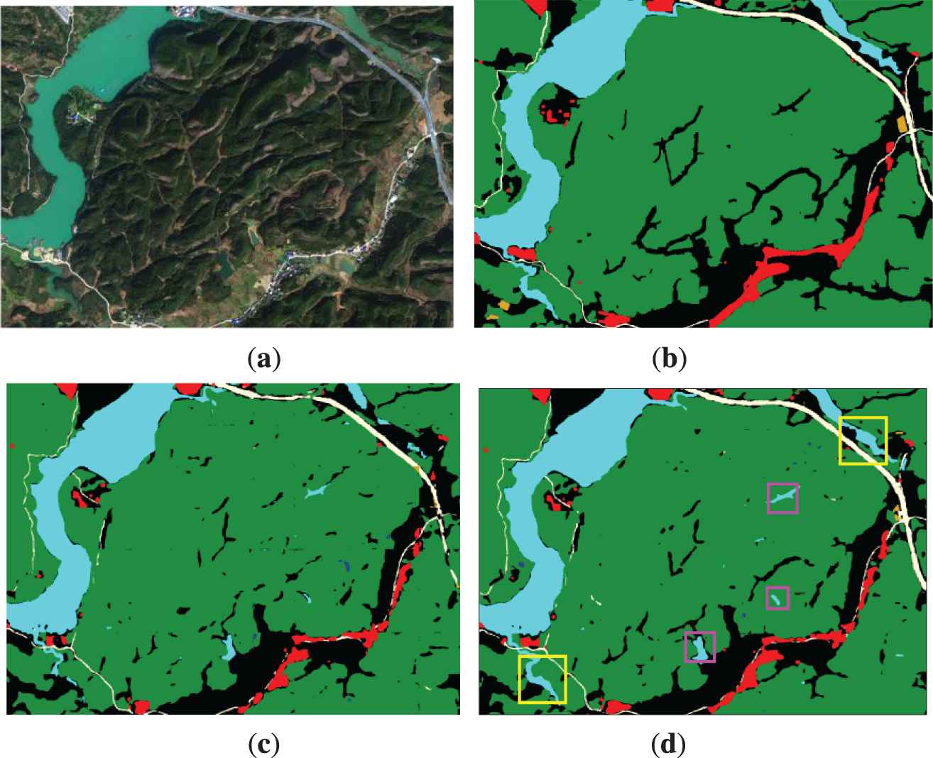
Prediction maps of the original FCN and dense fully convolutional network (DFCN). (a) original high-resolution remote sensing image, (b) the ground truth, (c) prediction map of the original FCN, and (d) prediction map based DFCN121.
6. CONCLUSIONS
In this paper, in order to complete the census of woodland in Chenzhou, we carried out remote sensing measurements on the terrain of the area and made a data set, and used deep learning methods to label woodland. We compared and analyzed the segmentation results of different classic semantic segmentation models on the remote sensing dataset of Chenzhou, and proposed the DFCN method to segment high-resolution remote sensing images for woodland labeling, and obtained the same dataset under the same experimental conditions. In the experiment, our data set was divided into 7 classes. However, the classification effect of two classes (bare land or wasteland, furrow) is not ideal, mainly due to the small number of samples of these two classes in training set. In addition, there may be some mixed labels when manually labeling the data set, which will affect the accuracy of experimental results.
The approach proposed in this paper has been applied in Chenzhou, China, to monitor the changes of woodland, rivers, and provide help for the development of forestry resources and the protection of the ecological environment. In the future work, we need to mark more data sets of forest classification with high quality, and study the new artificial intelligence classification method for woodland labeling, so as to find a segmentation model with more precision and efficiency.
CONFLICTS OF INTEREST
The authors declare no conflicts of interest.
AUTHORS' CONTRIBUTIONS
Conceptualization: W.W.; Methodology: Y.Y. and Y. H.; Software, Y.Y. and X.W.; Formal analysis: J.L.; Investigation: Y.L.; Writing—original draft preparation: W.W.
Funding Statement
This research was funded by National Defense Preresearch Foundation of China under Grant 7301506, National Natural Science Foundation of China under Grant 61070040, Scientific Research Fund of Hunan Provincial Education Department under Grant 17C0043, and Hunan Provincial Natural Science Fund under Grant 2019JJ80105, and Changsha Science and Technology Project “Intelligent processing method and system of remote sensing information for water environment monitoring in Changsha.”
DATA AVAILABILITY
The dataset used in the paper can be obtained by contacting Wei Wang (wangwei@csust.edu.cn).
REFERENCES
Cite this article
TY  - JOUR
AU  - Wei Wang
AU  - Yujing Yang
AU  - Ji Li
AU  - Yongle Hu
AU  - Yanhong Luo
AU  - Xin Wang
PY  - 2020
DA  - 2020/09/16
TI  - Woodland Labeling in Chenzhou, China, via Deep Learning Approach
JO  - International Journal of Computational Intelligence Systems
SP  - 1393
EP  - 1403
VL  - 13
IS  - 1
SN  - 1875-6883
UR  - https://doi.org/10.2991/ijcis.d.200910.001
DO  - 10.2991/ijcis.d.200910.001
ID  - Wang2020
ER  -