
Diagnosis of COVID-19 by Wavelet Renyi Entropy and Three-Segment Biogeography-Based Optimization
 , Chaosheng Tang1, *, , Xin Zhang3, *,
 Those authors contributed equally to this paper
- DOI
- 10.2991/ijcis.d.200828.001How to use a DOI?
- Keywords
- Wavelet Renyi entropy; three-segment biogeography-based optimization; feedforward neural network; COVID-19; diagnosis
- Abstract
Corona virus disease 2019 (COVID-19) is an acute infectious pneumonia and its pathogen is novel and was not previously found in humans. As a diagnostic method for COVID-19, chest computed tomography (CT) is more sensitive than reverse transcription polymerase chain reaction. However, the interpretation of COVID-19 based on chest CT is mainly done manually by radiologists and takes about 5 to 15 minutes for one patient. To shorten the time of interpreting the CT image and improve the reliability of identification of COVID-19. In this paper, a novel chest CT-based method for the automatic detection of COVID-19 was proposed. Our algorithm is a hybrid method composed of (i) wavelet Renyi entropy, (ii) feedforward neural network, and (iii) a proposed three-segment biogeography-based optimization (3SBBO) algorithm. The wavelet Renyi entropy is used to extract the image features. The novel optimization method of 3SBBO can optimize weights, biases of the network, and Renyi entropy order. Finally, we used 296 chest CT images to evaluate the detection performance of our proposed method. In order to reduce randomness and get unbiased result, the 10 runs of 10-fold cross validation are introduced. Experimental outcomes show that our proposed method is superior to state-of-the-art approaches in terms of sensitivity, specificity, precision, accuracy, and F1.
- Copyright
- © 2020 The Authors. Published by Atlantis Press B.V.
- Open Access
- This is an open access article distributed under the CC BY-NC 4.0 license (http://creativecommons.org/licenses/by-nc/4.0/).
1. INTRODUCTION
On February 11, 2020, WHO announced in Geneva, Switzerland, that the novel coronavirus pneumonia was named corona virus disease (COVID-19), referring to the pneumonia caused by the coronavirus 2019 infection. According to the existing statistical data, a small number of patients are accompanied by upper respiratory and digestive tract symptoms, e.g., nasal congestion, runny nose, and diarrhea [1]. To June 30, 2020, COVID-19 has affected more than 188 countries and regions around the world, with a total of 10,302,867 confirmed cases and 505,518 deaths.
The chest CT of COVID-19 patients shows patchy, flocculent, nodular, and exudative shadows in the subpleural area, which are usually dominated by double lower lungs according to the available chest CT data of COVID-19 patients. Ground glass opacity (GGO) was the main manifestation of the lesions. In critical patients, large fusion and mesh-like changes of GGO are observed [2]. Therefore, chest imaging is one of the common clues for the detection and diagnosis of COVID-19, and it is also an important focus for clinicians. For example, Pan et al. [3] found that the cause of the disease on lung computed tomography (CT) was positively correlated with the number of lesions, among which the median time point about 10 days after the onset was the most serious by CT score. Wang et al. [4] found from 93 cases of COVID-19 CT that 97.8% of patients’ lesions located in the pleura below. Ground glass shadows appeared in 74.2% of patients, and ground glass shadow detection in normal patients (79.5%) was higher than that in critically ill patients (55%). Consolidation shadows were present in 60.2% of patients, consolidation shadows detection in critically ill patients (90%) was higher than normal patients (52.1%). Bernheim et al. [1] concluded from the CT manifestations of 121 cases of COVID-19 that 17% of the patients had accumulated unilateral lung, the most common manifestation being ground glass shadow (which could be the only manifestation or coexisting with time-variant shadow), and only 2% of the patients had consolidation shadow on CT. In the 0–2 days after the onset, unilateral lung involvement was the most common. 56% of the patients presented normal CT appearance, 44% presented ground glass shadow, and 17% presented consolidation shadow. Both sides of the lungs were affected by 76% and 88% of patients 3–5 days after onset and 6–12 days after onset, respectively. Ground glass shadows were observed in 88% of the two groups, and consolidation shadows were observed in more than half of the patients [1]. Guan et al. [2] reported 840 cases of hospitalized patients with CT examinations, only 76.4% of the patients present with pneumonia, 50.0% and 46.0% of patients presented ground glass shadow and patchy shadow, respectively. Besides, local plaques were found in 37.2% of patients. In the case with a good treatment effect, the pulmonary CT performance gradually improved. In contrast, the pulmonary CT performance gradually worsened.
Recently, many researchers use computer vision and artificial intelligence to detect COVID-19, such as radial basis function neural network (RBFNN) [5], kernel-based extreme learning machine (KELM) [6], extreme learning machine with bat algorithm (ELMBA) [7]. Great progress has been achieved. However, in the course of performing the training algorithm of the classifier, they all face the situation of either falling into the local optimal [8,9] or failing to reach the global optimal.
To solve above issues, this study proposes a smart system to diagnose COVID-19 by using wavelet Renyi entropy (WRE) and 3SBBO. It will help clinicians make more accurate judgments on patients’ conditions and even provide automatic diagnosis.
There are scholars using deep learning techniques in detecting COVID-19, Rosebrock [10] presented a guide for using deep learning (Keras and TensorFlow) to detect COVID-19. This guide can help readers learn sample diseased and healthy X-ray images, train CNNs to detect COVID-19 automatically, and evaluate their results. Maghdid et al. [11] shared a low-cost technique of using smartphone-embedded sensors to diagnose COVID-19. This is particularly helpful since many people are currently holding smartphones every day. Wang and Wong [12] published a DL framework (COVID-Net), which was adapted for detecting COVID-19 patients based on chest radiography scans. The authors also used an explainable method to acquire more meaningful understandings into vital elements linked with COVID cases.
In this study, as the dataset is relatively small, we used WRE as feature descriptors and feedforward neural network (FNN) [13,14] as the classifier instead of the deep learning, which is widely used in biomedical image analysis. We believe that the order of WRE is of great significance for image feature detection. However, existing optimization algorithms can only optimize weights and biases of FNN, such as genetic algorithm (GA)[15] and biogeography-based optimization (BBO) [16]. Therefore, we proposed a novel three-segment biogeography-based optimization (3SBBO) that can not only optimize the order of Renyi entropy (RE), but also optimizes the weights and biases of FNN. In all, our contributions are composed of those points: (1) Introduce WRE extraction method and prove it is suitable for chest CT images. (2) Propose a 3SBBO algorithm to optimize RE order, weights and biases simultaneously. (3) Present a more effective automatic detection method for COVID-19 based on chest CT.
The rest of the paper is organized as follows: Section 2 describes the method of dataset selection. Section 3 explains wavelet decomposition and WRE, describes the construction of the classifier, the proposed optimization method: 3SBBO, and also gives the corresponding evaluation method. The experiment design is given in Sections 4 and 5 gives the experimental results and the discussion of the results. Section 6 concludes the work. Table 5 provides variable definition and Table 6 shows all the abbreviations used in this paper.
2. DATASET
Our experimental dataset consists of 296 images from chest CT, including 148 images were taken from COVID-19 patients (41 males and 25 females). The remaining 148 images were taken from healthy subjects (31 males and 35 females).
The 66 COVID-19 patients and 66 healthy subjects were examined using Philips Ingenuity 64 row spiral CT machine, KV: 120, MAS: 240. Healthy subjects were randomly selected from healthy people (tested negative). All subjects are in a supine position, with both upper limbs lifted up, and exposed with breath-holding after deep inhalation. The scanning range is from the thoracic inlet to the costal diaphragm angle. Using tube voltage 110–130 kV and automatic tube current technology, scanning layer thick layer spacing is 3 mm. Resolution of images are 1024
All the sampled images are transmitted to medical image PACS for observation, and the most representative image is selected by two doctors who are experienced in COVID-19 diagnosis based on the characteristics of the CT. The screen method is as follows: for COVID-19 patients, the layer with the largest lesion features is selected. For healthy subjects, the image level could be selected at will. When two doctors disagree about the diagnosis of an image, a senior doctor should be consulted to reach an agreement. In the preparation of the experiment, a summary of the dataset is shown in Table 1. We do not collect age information, since our focus is to identify COVID-19 from chest CT images.
| Set | COVID-19 | Healthy |
|---|---|---|
| No. of patients | 66 (41 males and 25 females) | 66 (31 males and 35 females) |
| No. of total images | 148 | 148 |
COVID-19, coronavirus disease 2019.
Statistics of dataset.
3. Methodology
Table 5 shows all variables used in this study, in order to ease the understanding of this paper. Table 6 gives the abbreviation and their full names.
3.1. Wavelet Decomposition
In order to decompose signals at different scales and targets, wavelet decomposition is introduced. In the wavelet decomposition process, the approximate subband represents the low frequency information of the signal, while the detail subband represents the high-frequency information of the signal.
For a particular signal/image, we use discrete wavelet transform (DWT) to transform that signal/image into the wavelet domain. DWT achieves multistage transformation by transmitting the previous approximation subband to the quadrature mirror filter (QMF). Compared with the standard Fourier transform, which has some disadvantages such as unintuitive representation and complex signal spectrum caused by noise, wavelet transform is advantageous in time/space resolution.
Set
Here, the
Here, the
In this way, DWT can be written as
Deep learning is a hot topic that can automatically learn features; nevertheless, the small size of our dataset does not work well on deep learning approaches. So, traditional feature engineering (feature extraction plus classification framework) was chosen in this study.
3.2. Two-Dimensional Wavelet Decomposition
Assuming a given image can be symbolized by
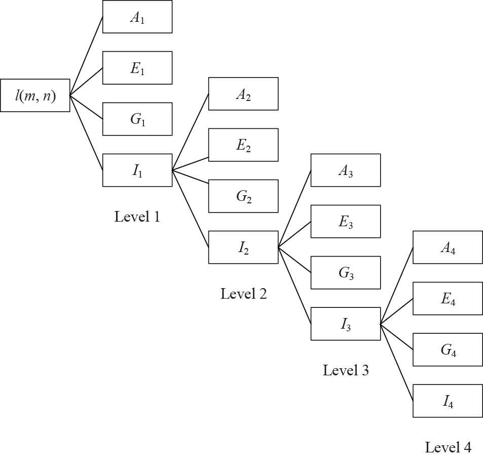
A toy example of a 4-level two-dimensional discrete wavelet transform (2D-DWT).
Subband I1 can be decomposed into four other subbands at the second level. Figure 1 presents a toy example of 4-level decomposition. This study chose to use 3-level decomposition. The reason why we use 3-level decomposition is by trial-and-error method.
Mathematically, assume
And subsequent decomposition as
3.3. Basics of RE
Each element of the wavelet decomposition subband can be regarded as a discrete random variable
Suppose the corresponding probability mass function (PMF) is
The
Here,
Figure 2 shows the RE of different
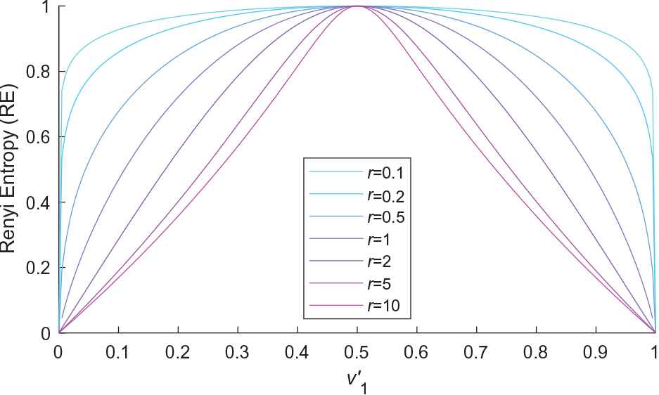
The Renyi entropy (RE) of various
It can be clearly seen that the concaveness and nonincreasing of
3.4. Feedforward Neural Network
To train the classifier, we propose an algorithm that combines the FNN with 3SBBO. The FNN consists of three layers: an input layer, hidden neuron layers, and an output neuron layer. The connection mode between the neurons of each layer is full connection. Figure 3 is the structural diagram of FNN.
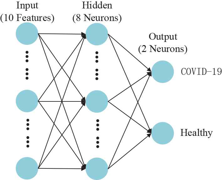
Structure diagram of feedforward neural network (FNN). (The structure if fixed by trial-and-error method)
In the experiment of this paper, we set the number of neurons in the hidden layer to 8 by manual trial-and-error. According to the general approximation theorem, FNN has powerful approximation ability, and it can approximate the corresponding expected output arbitrarily [19]. Although many classifiers such as support vector machine, decision tree, and naive Bayes are often used by some scholars in medical image analysis, the simple and practical FNN can better complete the difficult nonlinear mapping on the premise of less cost. Therefore, FNN is one of the network models of great significance and wide application in the field of medical image analysis.
Remember we use 3-level decomposition, so we will have
The size of hidden neuron is determined as 8, so the hidden layer output is defined as
The output of FNN can be expressed as
Since we have to handle a binary classification in this study. Using simple math, we can update above two equations in matrix form as
For any given function
3.5. Standard BBO
BBO is an optimization algorithm with both good local and global solutions, which can show good convergence in image classification. There are many other excellent algorithms [20–27], which we will use into our task in the future.
3.5.1. Concepts of BBO
Figure 4 shows the corresponding relationship between BBO, GA, and problem. In which, the ecosystem in BBO corresponds to population in GA, both of which represent the solution set of a problem. Habitat in BBO corresponds to individuals in GA, and they all represent a solution in a problem solution set. HSI in BBO corresponds to fitness in GA, they both represent the objective function of a problem. SIV in BBO corresponds to GA, they all represent variable in a problem [28].
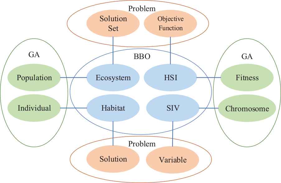
The relationship among genetic algorithm (GA) genetic algorithm genetic algorithm and biogeography-based optimization (BBO) and problem space.
To accurately describe biogeographic models, we will introduce the terms as follows: habitat, where species live and reproduce, to describe candidate solutions to the problem to be solved. Habitat suitability index (HSI), which measures the number of species in a habitat and describes the practicality of a candidate solution. Suitability index variable (SIV), which measures the habitability of a habitat and is used to adjust the practicality of a candidate solution. Among them, migration operation and mutation operation are the main steps of BBO algorithm in optimizing specific problems. At the same time, the introduction of elitism solves the problem of saving better solutions in the process of BBO algorithm. Figure 5 shows the species migration diagram of BBO algorithm.
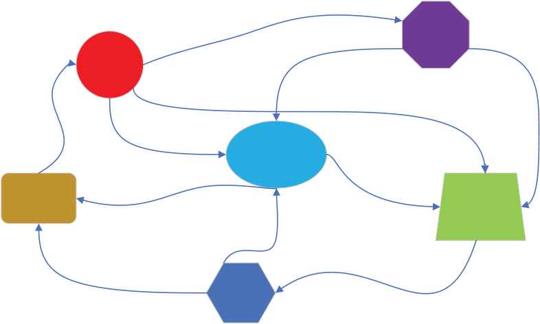
Diagram of biogeography-based optimization (BBO) habitat and migration. (The geometric shapes represent habitats, and the arrows represent migrations)
3.5.2. Migration operation
The migration operation of BBO algorithm mainly depends on the migration operator. Species migrate from habitats with a higher value of HSI to habitats with a lower value of HSI [29]. Therefore, the following formula can be obtained:
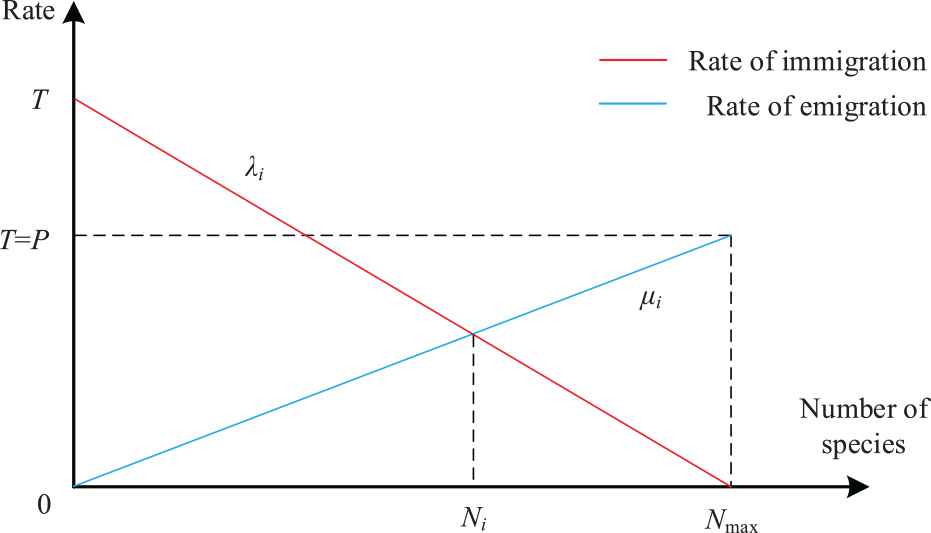
Linear model of population migration.
Considering that the maximum immigration rate P is equal to the maximum emigration rate T, it can be expressed as
3.5.3. Mutation operation
BBO algorithm will select some habitats with low HSI value to perform mutation operation. Habitat optimization is achieved by changing a single SIV to facilitate migration of species. Thus, the number of species in a habitat is closely related to the probability of mutation. This leads to the following update formula:
Here,
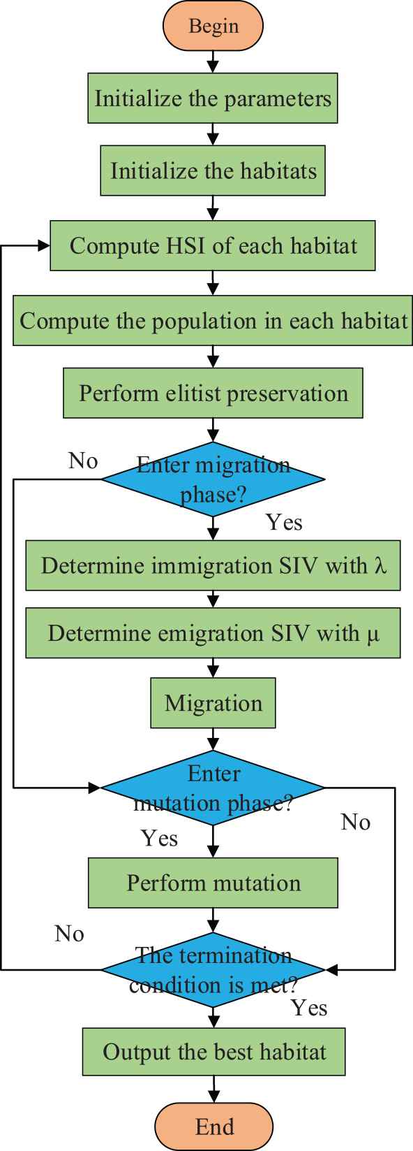
Flowchart of biogeography-based optimization (BBO) method.
3.6. Proposed Three-Segment BBO (3SBBO)
3SBBO can optimize of the RE order, weights and biases simultaneously by combining three-segment encoding strategy with the advantages of BBO, e.g., fast convergence speed, fewer algorithm parameters, and strong global search ability.
3.6.1. Rational of 3SBBO
The standard BBO algorithm optimizes the weights and bias of FNN by performing migration operations and mutation operations. However, we believe that RE order is also an important parameter affecting WRE feature extraction performance under the premise of fixing the number of FNN hidden layer neurons. Therefore, we propose the 3SBBO designed to simultaneously optimize RE order, weights, and bias.
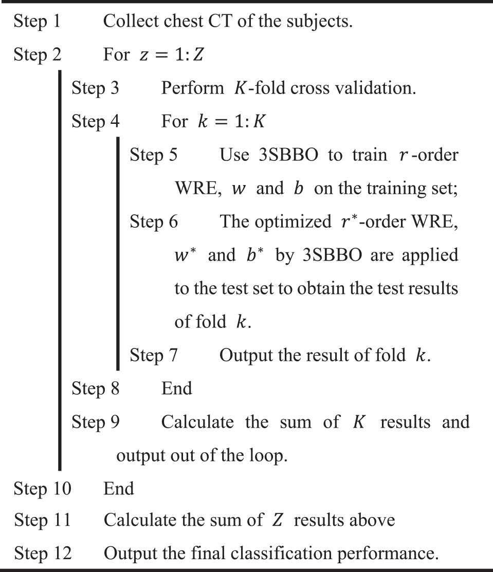
Figure 8 is the flow chart of our method. We will collect chest CT of the subjects and then conduct
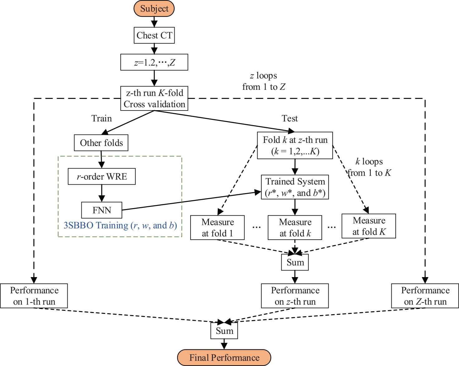
The flowchart of proposed three-segment biogeography-based optimization (3SBBO) method.
 |
Pseudocode of three-segment biogeography-based optimization (3SBBO).
On the training set, 3SBBO is used to optimize the RE order, weights, and biases. (ii) The optimized
3.6.2. Encoding of 3SBBO
To optimize our task, the variable
Here,
The total population can be written as
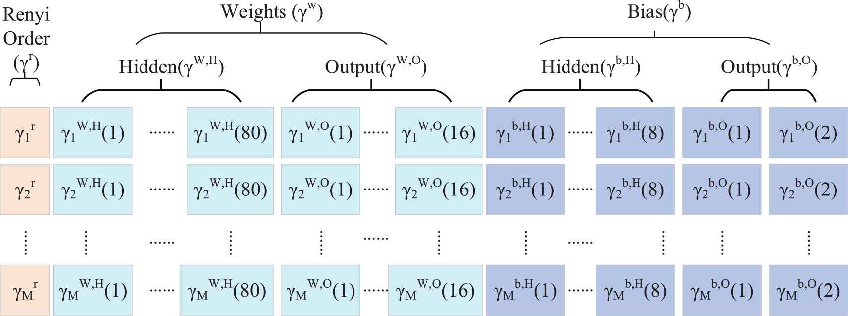
Encoding of habitat and ecosystem.
4. EXPERIMENTAL DESIGN
4.1. 10 Runs of 10-Fold CV
In this paper, in order to prevent overfitting, 10-fold CV is introduced. CV is a strict statistical validation technique widely used in many academic fields, such as harmonic approximation [30], ferromagnetic resonance [31], etc. The specific implementation method is as follows: the experimental dataset is randomly divided into 10 equal parts, numbered from 1 to 10. First, set the fold No.1 as the test set, the remaining folds as the training set. Then set the fold No. 2 as the test set, and the remaining folds as the training set. Take turns to set the fold No. 3 through No. 10 as test set, and set the remaining dataset as training set in each turn. Figure 10 shows an example of one run of 10-fold CV on our dataset of 296 images.

Illustration of one run of 10-fold cross validation.
Finally, the sum value of the test results of the above 10 folds is obtained, so as to evaluate the performance of proposed algorithm. To make a more accurate assessment of the accuracy of algorithm, we will carry out 10-fold CV 10 times.
In this experiment, the deal confusion matrix
The ideal confusion matrix for 10-fold CV 10 times is
4.2. Indicators
To assess the confusion matrix for the 10-fold CV, we set COVID-19 patients as positive class and healthy subjects as negative class. During the assessment, true positive (TP) was defined as identified COVID-19 patients correctly, true negative (TN) as identified healthy subjects correctly, false positive (FP) as healthy subjects were wrongly predicted to be COVID-19 patients, and false negative (FN) as COVID-19 patients were wrongly predicted to be healthy subjects.
According to the confusion matrix, six metrics were defined:
Here, the value of
The value of
5. Experiment Results and Discussions
The parameters of this study were set by trial-and-error method and described below. Wavelet decomposition level = 3; Number of hidden heurons = 8; Maximum iterative epochs = 500; Population size = 20; Maximum emigration rate = Maximum immigration rate = 1; Maximum mutation rate = 0.1.
5.1. Wavelet Decomposition
Figure 11 is a sample of CT wavelet decomposition of the lungs of COVID-19 patients and healthy subjects, where, (b) and (d) are the 3-level decomposition of (a) and (c), respectively. We can clearly see that in the CT images of the lungs of COVID-19 patients, the shape of both lungs on tends to be round, and the apex of the upper lobe of the right lung has visible patchy ground glass shadow, which is in sharp contrast to the CT images of the lungs of healthy subjects. At the same time, this phenomenon can be observed more clearly in the picture after the 3-level decomposition.
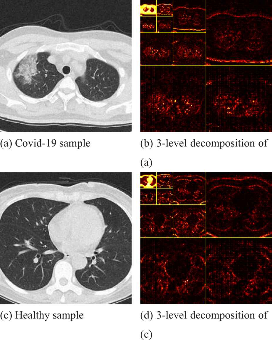
Two samples of wavelet decomposition.
5.2. Comparison of BBO with Other Optimization Algorithms
We compared our 3SBBO with traditional GA [15] and standard BBO [16]. The detailed results of every run are shown in Table 3.
| GA [15] |
||||||
|---|---|---|---|---|---|---|
| Run | Sen | Spc | Prc | Acc | F1 | MCC |
| 1 | 77.00 | 81.10 | 80.30 | 79.07 | 78.59 | 58.19 |
| 2 | 77.00 | 78.29 | 78.62 | 77.71 | 77.64 | 55.58 |
| 3 | 78.38 | 73.71 | 75.02 | 76.02 | 76.60 | 52.20 |
| 4 | 77.67 | 81.05 | 80.41 | 79.36 | 78.99 | 58.78 |
| 5 | 82.43 | 76.90 | 78.60 | 79.74 | 80.35 | 59.66 |
| 6 | 79.81 | 83.10 | 82.58 | 81.43 | 81.05 | 63.06 |
| 7 | 79.00 | 79.05 | 79.03 | 79.05 | 78.98 | 58.11 |
| 8 | 76.33 | 81.81 | 80.97 | 79.06 | 78.49 | 58.35 |
| 9 | 78.38 | 77.67 | 77.88 | 78.03 | 78.10 | 56.08 |
| 10 | 77.00 | 75.05 | 75.53 | 76.02 | 76.22 | 52.10 |
| Mean±SD | 78.30±1.71 | 78.77±2.88 | 78.89±2.23 | 78.55±1.58 | 78.50±1.42 | 57.21±3.18 |
| BBO [16] |
||||||
| Run | Sen | Spc | Prc | Acc | F1 | MCC |
| 1 | 80.43 | 77.71 | 78.32 | 79.06 | 79.27 | 58.28 |
| 2 | 83.05 | 81.76 | 81.87 | 82.43 | 82.29 | 65.08 |
| 3 | 81.76 | 80.38 | 81.03 | 81.08 | 81.29 | 62.30 |
| 4 | 77.71 | 85.76 | 84.58 | 81.75 | 80.94 | 63.76 |
| 5 | 83.76 | 71.57 | 74.72 | 77.70 | 78.94 | 55.85 |
| 6 | 79.00 | 82.48 | 82.39 | 80.76 | 80.48 | 61.78 |
| 7 | 83.14 | 84.48 | 84.27 | 83.82 | 83.61 | 67.78 |
| 8 | 83.14 | 80.43 | 81.13 | 81.78 | 82.05 | 63.70 |
| 9 | 79.71 | 79.05 | 79.21 | 79.39 | 79.46 | 58.77 |
| 10 | 81.76 | 81.14 | 81.42 | 81.44 | 81.49 | 63.04 |
| Mean±SD | 81.35±1.94 | 80.48±3.73 | 80.89±2.76 | 80.92±1.69 | 80.98±1.41 | 62.03±3.35 |
| 3SBBO (Ours) |
||||||
| Run | Sen | Spc | Prc | Acc | F1 | MCC |
| 1 | 84.43 | 79.81 | 80.90 | 82.12 | 82.48 | 64.56 |
| 2 | 87.14 | 88.48 | 88.50 | 87.82 | 87.78 | 75.71 |
| 3 | 89.86 | 87.86 | 88.11 | 88.86 | 88.95 | 77.77 |
| 4 | 85.81 | 82.43 | 83.14 | 84.13 | 84.41 | 68.34 |
| 5 | 89.81 | 87.76 | 88.74 | 88.82 | 88.98 | 78.22 |
| 6 | 91.19 | 87.81 | 88.77 | 89.54 | 89.82 | 79.37 |
| 7 | 85.14 | 85.76 | 85.74 | 85.47 | 85.42 | 70.97 |
| 8 | 82.43 | 83.10 | 83.08 | 82.77 | 82.63 | 65.69 |
| 9 | 81.76 | 84.48 | 84.03 | 83.13 | 82.86 | 66.30 |
| 10 | 86.48 | 90.62 | 90.39 | 88.53 | 88.28 | 77.30 |
| Mean±SD | 86.40±3.00 | 85.81±3.14 | 86.14±3.03 | 86.12±2.75 | 86.16±2.77 | 72.42±5.55 |
Sen, Sensitivity; Spc, Specificity; Prc, Precision; Acc, Accuracy; MCC, Matthews correlation coefficient; GA, genetic algorithm; three-segment biogeography-based optimization (3SBBO); BBO, biogeography-based optimization.
Comparison with other optimization algorithms.
All indicators in Table 3 reflected that GA had the worst optimization effect, obtaining the worst performance. BBO had the better optimization results than GA, and obtained better indicator results. Finally, the proposed 3SBBO yielded the best optimization performance with the greatest measuring performance. Compared to GA, BBO improved the performance of each indicator by about 2%–5%. While 3SBBO improves the performance of each indicator by about 8%–12% compared to those of GA.
5.3. Comparison to State-of-the-Art Algorithms
We compared our 3SBBO algorithm with state-of-the-art approaches: RBFNN [5], KELM [6], ELMBA [7]. As shown in Table 4 and Figure 12, RBFNN, KELM and ELMBA use hold-out validation and our method uses 10
| Appr | VD | Sen | Spc | Prc | Acc | F1 | MCC |
|---|---|---|---|---|---|---|---|
| RBFNN [5] | HO | 65.91 | 75.00 | 72.50 | 70.45 | 69.05 | – |
| KELM [6] | HO | 56.82 | 61.36 | 59.52 | 59.09 | 58.14 | – |
| ELMBA [7] | HO | 55.00±2.58 | 76.36±2.44 | 69.97±2.44 | 65.68±1.92 | 61.56±2.25 | – |
| 3SBBO (Ours) | 10x10 fold CV | 86.40±3.00 | 85.81±3.14 | 86.14±3.03 | 86.12±2.75 | 86.16±2.77 | 72.42±5.55 |
(- means not available, Appr means approach, VD means validation, HO means hold-out, CV means cross validation)
Sen, Sensitivity; Spc, Specificity; Prc, Precision; Acc, Accuracy; MCC, Matthews correlation coefficient.
Comparison of state-of-the-art approaches in detecting COVID-19.
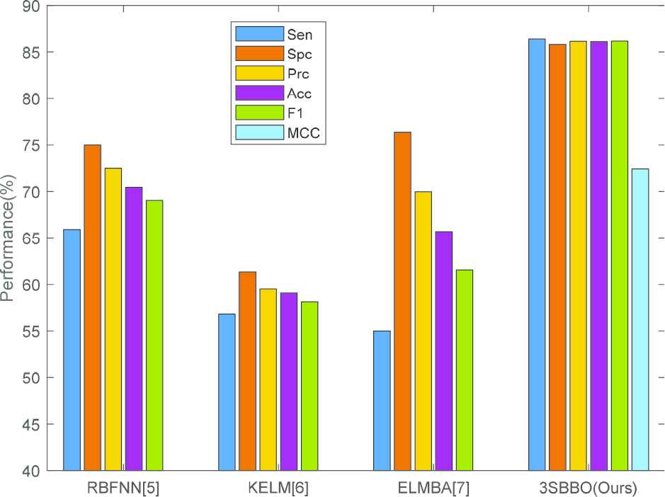
Bar plot of comparison results.
6. Conclusions
In this paper, we propose a computer vision-based diagnosis method based on WRE and the proposed 3SBBO. The method consists of three parts: WRE as feature extractor, FNN as classifier, and 3SBBO algorithm as optimizer. As can be seen through the experiment, after 10 times 10-fold CV, the MCC value of our method is 72.42
The disadvantages of this proposed smart COVID-19 diagnosis system are 2-fold: firstly, the WRE was extracted, we will attempt to test other effective features. Secondly, we will try to improve BBO, such as speed up the convergence speed of BBO algorithm and get a better global optimal solution.
In future studies, based on the differences between chest CT of COVID-19 patients and common pneumonia patients, the chest CT of COVID-19 patients where mesh shadow is more common in the lungs and boundaries are clearer. And chest CT of common pneumonia patients, where nodules of internal consolidation and thickening of bronchial wall are more common, with blurred boundaries. We will conduct a classification study of chest CT diagnosis of COVID-19 patients and common pneumonia patients based on computer vision. Second, we will develop a classifier based on multisource data, so that it can be applied to face recognition, alcoholism detection, and spectrum data. Third, we will try to collect more data and test the deep learning method.
CONFLICTS OF INTEREST
The authors declare that there is no conflict of interest.
AUTHORS' CONTRIBUTIONS
Shuihua Wang proposed the idea, Xiaosheng Wu and Chaosheng Tang implemented the algorithms. Xin Zhang drafted the paper and checked the experiment result. Shuihua Wang and Yudong Zhang drafted the paper and gave critical revisions. All authors approved the submission of the work.
ACKNOWLEDGMENTS
This paper was partially supported by Henan Key Research and Development Project (182102310629); Guangxi Key Laboratory of Trusted Software (kx201901); Royal Society International Exchanges Cost Share Award, UK (RP202G0230); Medical Research Council Confidence in Concept Award, UK (MC_PC_17171); Hope Foundation for Cancer Research, UK (RM60G0680); Fundamental Research Funds for the Central Universities (CDLS-2020-03); Key Laboratory of Child Development and Learning Science (Southeast University), Ministry of Education.
Appendix
The rest of the paper is organized as follws: Section 2 describes the method of dataset selection. Section 3 explains wavelet decomposition and WRE, describes the construction of the classifier, the proposed optimization method: 3SBBO, and also gives the corresponding evaluation method. The expriment design is given in Section 4 and 5 gives the experimental results and the discussion of the results. Section 6 concludes the work. Table 5 provides variable definition and Table 6 shows all the abbreviations used in this paper.
| VN | Variable Meaning |
|---|---|
| Section 3.1 |
|
| A given one-dimension signal. | |
| Coefficient of wavelet decomposition. | |
| Scale factor in wavelet decomposition. | |
| Translation factor in wavelet decomposition. | |
| Mother wavelet. | |
| Index of time. | |
| Value of translation factor in wavelet decomposition. | |
| Value of scale factor in wavelet decomposition. | |
| Approximate subband of wavelet decomposition. | |
| Detail subband of wavelet decomposition. | |
| Down-sampling. | |
| Low-pass filter in wavelet decomposition. | |
| High-pass filter in wavelet decomposition. | |
| Discrete form of the time variable t. | |
| Section 3.2 |
|
| An image. | |
| Horizontal quadrant subband. | |
| Vertical quadrant subband. | |
| Diagonal quadrant subband. | |
| Approximate component subband. | |
| 2D DWT operation. | |
| Section 3.3 |
|
| Value of the discrete random variables. | |
| Discrete random variable. | |
| A specified binary random variable. | |
| Probability of |
|
| Order of Renyi entropy. | |
| h | Index of possible value of Q. |
| H | Number of possible values of Q. |
| Section 3.4 |
|
| Output values of FNN (different values correspond to different labels (COVID-19, healthy)). | |
| Biases in FNN. | |
| Weights in FNN. | |
| Input vector. | |
| Y | Output of hidden layer. |
| O | Output of output layer. |
| Target output. | |
| An arbitrarily small number. | |
| Section 3.5 |
|
| Immigration rate of habitat with |
|
| Emigration rate of habitat with |
|
| Maximum rate of immigration. | |
| P | Maximum rate of emigration. |
| Number of species. | |
| Maximum number of species. | |
| Probability of performing mutation operations in a habitat with a species number of |
|
| Maximum rate of mutation. | |
| Probability that the habitat has the number of |
|
| Probability of maximal species. | |
| M | Number of habitats |
| Section 3.6 |
|
| Optimized biases of FNN. | |
| Optimized order of Renyi entropy. | |
| Optimized weights of FNN. | |
| Index of fold used as test set. | |
| Number of folds for cross validation. | |
| Candidate for weights of hidden layer to be optimized. | |
| Candidate for weights of hidden output to be optimized. | |
| Candidate for biases of hidden layer to be optimized. | |
| Candidate for biases of hidden output to be optimized. | |
| Order of Renyi entropy to be optimized. | |
| Set of weights to be optimized in FNN. | |
| Set of biases to be optimized in FNN. | |
| Section 4 |
|
| Confusion matrix. | |
| Run index (each run carries out a |
|
| Total number of runs. | |
(VN means variable name)
Variable definition table.
| Abbreviation | Full Definition |
|---|---|
| DWT | Discrete Wavelet Transform |
| QMF | Quadrature Mirror Filter |
| FNN | Feedforward Neural Network |
| BBO | Biogeography-Based Optimization |
| 3SBBO | Three-Segment BBO |
| HSI | Habitat Suitability Index |
| SIV | Suitability Index Variable |
| 3S | Three-Segment |
| TP | True Positive |
| TN | True Negative |
| FP | False Positive |
| FN | False Negative |
| MCC | Matthews Correlation Coefficient |
| GA | Genetic Algorithm |
| RE | Renyi Entropy |
| BRV | Binary Random Variable |
| CV | Cross Validation |
| PMF | Probability Mass Function |
Abbreviation table.
REFERENCES
Cite this article
TY  - JOUR
AU  - Shui-Hua Wang
AU  - Xiaosheng Wu
AU  - Yu-Dong Zhang
AU  - Chaosheng Tang
AU  - Xin Zhang
PY  - 2020
DA  - 2020/09/17
TI  - Diagnosis of COVID-19 by Wavelet Renyi Entropy and Three-Segment Biogeography-Based Optimization
JO  - International Journal of Computational Intelligence Systems
SP  - 1332
EP  - 1344
VL  - 13
IS  - 1
SN  - 1875-6883
UR  - https://doi.org/10.2991/ijcis.d.200828.001
DO  - 10.2991/ijcis.d.200828.001
ID  - Wang2020
ER  -