
Quantum Behavior-Based Enhanced Fruit Fly Optimization Algorithm with Application to UAV Path Planning
 , Shuang Xia1, 2, 4, Xiuzhi Li1, 2, 4
- DOI
- 10.2991/ijcis.d.200825.001How to use a DOI?
- Keywords
- Fruit fly optimization algorithm; Continuous function optimization; Delta potential well; Quantum behavior; Path planning
- Abstract
As a newly developed simple and effective optimization technology, the fruit fly optimization algorithm (FOA) has been successfully applied in many fields. To accelerate the algorithm convergence and avoid the local optimum, the enhanced FOA based on quantum theory called QFOA is proposed in this paper. When establishing the quantum Delta potential well around the location of fruit fly swarm, QFOA introduces the quantum behavior-based searching mechanism into the original osphresis-based search procedure of FOA. In the process that fruit flies find and move toward the food source, fruit flies follow the wave function property of the Delta potential well rather than the Newtonian mechanics. Taking advantage of the probability and uncertainty of quantum theory, the proposed QFOA can effectively overcome the weakness in premature convergence and easy trapping into local optimum. Since there are two popular models of the basic FOA, this paper also develops two corresponding QFOAs. Experimental results on various benchmark functions show that both the two QFOA models has overall better performance compared with the basic FOA as well as other FOA variants and other well-known optimization algorithms. In addition, the proposed QFOAs are also applied to unmanned aerial vehicle (UAV) path planning problem in the three-dimensional environment, and comparative results about the obtained optimal flight path and population convergence process show the effectiveness of QFOAs.
- Copyright
- © 2020 The Authors. Published by Atlantis Press B.V.
- Open Access
- This is an open access article distributed under the CC BY-NC 4.0 license (http://creativecommons.org/licenses/by-nc/4.0/).
1. INTRODUCTION
The complex continuous optimization problem, which is to find the optimal solution that fulfills a set of constraints and achieves the maximum or minimum value of the function [1], is a universal issue, in many mathematical and engineering fields, such as automatic control, decision-making, signal processing, etc. Many traditional optimization techniques, which often use the gradient strategy, are applied to these problems, such as the integer programming, gradient descent methods, linear programming, and dynamic programming [2]. They are usually based on the single initial individual solution and will achieve the same local solutions when starting from the same initial individual. When dealing with complex practical problems that generally have high dimension, or multiple constraints, or multimodal [3], these traditional optimization techniques easily lead to the high computational complexity and even fail to determine the optimal solutions. To solve the complex optimization problems, population-based intelligent optimization techniques, which usually search for the feasible solution in some random fashion with starting from the initial solution set, have emerged and show their advantages in terms of calculate precision and time complexity [4,5]. These intelligent optimization techniques are generally inspired by the biological social behavior, such as ant colony optimization (ACO) [6], particle swarm optimization (PSO) [7], artificial bee colony (ABC) optimization [8], firefly algorithm (FA) [9], etc., and the evolution process in nature, including differential evolution (DE) algorithm [4,10], genetic algorithm (GA) [11], etc., as well as the physical or chemical phenomenon, such as chemical reaction optimization (CRO) algorithm [12], gravitational search algorithm (GSA) [13], biogeography-based optimization (BBO) [14] algorithm, etc.
The fruit fly optimization algorithm (FOA) is another newly proposed population-based intelligent optimization technique [15], which is originally inspired by the food-finding behavior of fruit flies. FOA is not only very effective to solve complex optimization problems, but also more simple and easy to implement than other existing population-based algorithms [16]. Firstly, the procedure of FOA only takes several lines to code the core part of the algorithm in any programming language. Secondly, FOA has no other additional control parameters besides the maximum number of iteration and population size. Therefore, FOA has widely attracted the attention of many researchers from various fields, including path planning [16,17], flowshop rescheduling [18], multi-dimensional knapsack problem [19], parameter identification [20], controller parameter tuning [21], etc.
FOA has simple operation and acceptable searching capability, however, it also has some shortcomings of the premature convergence and slow convergent speed during the later evolution process. To overcome these shortcomings as well as improve the search efficiency and global search capability, various improved FOA variants have been put forward by researchers [1, 16, 18-20,22-26]. The improved fruit fly optimization (IFFO) algorithm [1] introduces a new parameter to adaptively control the search scope around the fruit fly swarm location and a new solution generating method to enhance the accuracy and convergence rate. The phase angle-encoded FOA with mutation adaptation mechanism (θ-MAFOA) [12] adopts the mutation adaptation mechanism to enhance the balance between the exploitation and exploration ability of the basic FOA, and besides, the phase angle-based-encoded strategy for fruit fly locations is also adopted to achieve the better convergence performance. In the chaotic-enhanced fruit fly optimization algorithm (CFOA) [20], the chaotic sequence is employed to enhance the global optimization capacity of the original FOA. In the multi-swarm fruit fly optimization algorithm (MFOA) [24], several sub-swarms move independently in the search space at the same time and local behavior rules between sub-swarms are employed to explore global optimal. All these improved FOA variants succeed in overcoming the drawback of the original FOA to some degree. However, for the FOA variants, there is still much room for improvement to achieve better performance in terms of either convergence speed or avoiding to trap into the local optimum, especially for the complex practical problems. Generally, the population diversity and the search randomness play the crucial roles in the population-based optimization techniques. In this paper, we proposed the quantum-behaved FOA (QFOA) model, with the purpose that try to take advantage of the uncertainty of quantum theory to further enhance the performance of FOA by enabling fruit flies to have the quantum behavior. Especially, for the two popular standard FOA models in the literatures, two QFOA models are both presented accordingly, as well as the implement processes.
The idea behind quantum theory, of which the theoretical basis is the classical quantum mechanics, is to hijack some of the “spookiness” in the area of physics known as quantum behavior mechanism [27]. For the population-based optimization techniques, solutions can usually show the higher diversity, which helps to achieve the powerful searching capability, when moving according to the quantum behavior rule. For example, the quantum-behaved particle swarm optimization (QPSO) makes particles move following quantum mechanics rather than Newtonian mechanics, and thus, help to enhance the particle’s ability of jumping out of the local optimum [28,29]. The quantum firefly algorithm (QFA) integrates quantum theory into the basic FA and succeed in overcoming the loss of diversity [30].
In this paper, we introduce the quantum theory into the original FOA to achieve more effective performance. In the enhanced FOA, we assume that the fruit flies locate in a quantum world and the Delta potential well exists around the location of fruit fly swarm. When moving in the space to search for the food, fruit flies follow the quantum mechanics and their behaviors have the uncertainty as the wave function. The quantum-behaved strategy can effectively avoid the premature convergence and improve the escaping ability from the local optimum. Numerical results on benchmark functions reveal that the proposed FOA models are superior to the standard FOA models and other FOA variants as well as some state-of-the-art population-based techniques. Then, we apply the proposed QFOA models to the practical complex problem that finds the optimal flight path for unmanned aerial vehicle (UAV) in the three-dimensional (3D) terrain environments with various enemy weapons. Numerical experiments are carried out on various test scenarios and the results show the effectivity of our proposed QFOA models.
The rest of this paper is organized as follows: Overview of the basic FOA is described in Section 2, including common descriptions of two FOA models. Section 3 presents detailed statement and implement process for the models of the proposed QFOA variants. In Section 4, the comparison and simulation results on several benchmark functions are studied. Section 5 presents the application of the proposed QFOA models to the UAV path planning. Experimental results of path planning are shown in Section 6. Section 7 concludes this paper finally.
2. STANDARD FOA MODELS
FOA is a new population-based algorithm for searching global optimization based on the foraging behavior of fruit flies [11]. Fruit flies are superior to other species in terms of olfactory and visual senses. By using their osphresis, fruit flies can find all types of scents floating in the air and explore the direction of food source. After that, fruit flies can find the food source when getting close to the location of food by using their vision.
According to the foraging characteristics of the fruit fly swarm, FOA can be divided into three consecutive operations, namely swarm location initialization, osphresis-based search, and vision-based search. As to the detailed implementation, existing literatures give two different types of mathematical models to describe the three operations, which are summarized and recorded as FOA-1 and FOA-2 in this paper. Both the two FOA models will be described in the following section:
Without loss of generality, the global optimization problem in the continuous domain can be summarized as follows:
2.1. FOA-1 Model
In 2012, W.T. Pan put forward the basic idea of FOA for the first time [15], and meanwhile, the complete mathematical model was given to describe the three operations of FOA. In this type of FOA model, the decision variable is encoded as the reciprocal of the distance between the fruit fly location and the origin. To avoid confusion, the FOA model appearing in Refs. [9,15,17,19], is recorded as FOA-1, of which the operations are described as follows:
Swarm location initialization
Set the population size Mosp and the maximum number of iterations Gmax, and then, the fruit fly swarm location (Xaxis, Yaxis) is randomly initialized in the decision space as
Osphresis-based search
In the osphresis-based search process, the fruit fly swarm generate Mosp new locations of the food source that are randomly around the current location of the fruit fly swarm. The random searching strategy using the osphresis to find the new food location is given by
For every location generated by the osphresis-based searching strategy, its smell concentration judgment Si is the reciprocal of the distance between the location and the origin, as follows:
Actually, the smell concentration judgment corresponds to the candidate solution of the objective function in the decision space. The value of the objective function for the candidate solution, which corresponds to the smell concentration of the food source for the smell concentration judgment, is calculated as follows:
Vision-based search
The vision-based searching process of the fruit fly swarm is essentially a greedy selection procedure. The fruit fly swarm observe all the locations generated via the above osphresis-based searching process and select the best location with the minimum smell concentration, as follows:
The best smell concentration Smellindex is compared with Smellaxis of the fruit fly swarm location (Xaxis, Yaxis). If Smellindex< Smellaxis, then the fly swarm will fly toward the new location by using vision and (Xaxis, Yaxis) will be replaced by (Xindex, Yindex). The vision-based search can be described as follows:
The osphresis-based and vision-based searching processes are repeated until the stopping criterion is satisfied. The general procedure of abovementioned operations is shown in Algorithm 1.
Algorithm 1: Procedure of FOA-1
/* Initialization*/
1. Set the generation counter g = 0;
2. Set the number of fruit flies as Mosp;
3. Randomly initialize the fruit fly swarm’s location as [Xaxis, Yaxis];
/* Iterative search*/
4. while termination criteria is not satisfied do
5. Generation counter g = g + 1
/* Search using osphresis */
6. for i = 1: Mosp do
7. Generate the random direction and distance as:
Xi = Xaxis + random, Yi = Yaxis + random
8. Compute the distance to the origin as:
9. Calculate judged value of smell concentration as: Si= 1/Di
10. Evaluate the smell concentrations as: Smelli = f(Si)
11. end for
/* Search using vision */
12. Select the fruit fly that has the best smell concentration:
index = arg max(Smelli)
13. if [Xindex, Yindex] has the better smell than [Xaxis, Yaxis], then
14. Xaxis = Xindex and Yaxis = Yindex
15. end while
2.2. FOA-2 Model
In addition to the above FOA-1 model, there existing another popular mathematical model to describe operations of FOA [1,23], which is recorded as FOA-2 in this paper. The FOA-2 model codes the decision variable using the floating number directly and can be adapted to solve the high-dimensional functions [1]. The operations of FOA-2 model are described as follows:
Swarm location initialization
Firstly, the fruit fly swarm location xaxis = [xaxis,1, xaxis,2, …, xaxis,D] is randomly initialized as
Osphresis-based search
In the osphresis-based search process, the Mosp new locations are randomly generated around the current swarm location as
Then, the smell concentration is calculated as follows:
Vision-based search
The vision-based searching process of the fruit fly swarm is essentially a greedy selection procedure. That is, the fruit fly swarm observer all the locations generated via the above osphresis-based searching process and find out the best location that has the minimum smell concentration, as follows:
Compare the best smell concentration Smellindex with the smell concentration Smellaxis of the current swarm location xaxis. If
General procedure of the FOA-2 model is shown in Algorithm 2.
Algorithm 2: Procedure of FOA-2
/* Initialization */
1. Set the generation counter g = 0;
2. Set the number of fruit flies as Mosp;
3. Randomly initialize xaxis = [xaxis,1, xaxis,2, …, xaxis,D] with [Xmin, Xmax]D;
/* Iterative search */
4. while termination criteria is not satisfied do
5. Generation counter g = g + 1
/* Search using osphresis */
6. for i = 1: Mosp do
7. Generate random location as xij= xaxis, j + random, j = 1,2,…D
8. if xij> Xmax, then
9. xij= Xmax
10. if xij< Xmin, then
11. xij= Xmin
12. Evaluate smell concentrations Smelli = f(xi), xi= [xi1, xi2,…, xiD]
13. end for
/* Search using vision */
14. Select the fruit fly that has the best smell concentration:
index = arg max(Smelli)
15. if f(xindex) < f(xaxis), then
16. xaxis = xindex
17.end while
3. QUANTUM-BEHAVED FOA MODELS
Based on the quantum theory, the fruit fly swarm are assigned to move in the quantum multi-dimensional space. The Delta potential well model is established to increase the uncertainty that the fruit fly sense and move to the food.
3.1. Quantum Delta Potential Well
According to the quantum theory [28], objects are described by the wave function ψ(x, t), rather than the position x and velocity v. Any quantum object has the wave-like properties and can exist in many places at once. In the quantum space, the probability of the object appearing on a spot is proportional to the strength module of the wave function on this spot, as follows:
According to the quantum physics, the motion of objects is described by the Schrödinger’s equation as follows:
3.2. Quantum Behavior of Fruit Flies
Hypothesize the fruit fly swarm move in the quantum space, and fruit flies search for the food source in the Delta potential well. In the quantum space, the foraging and random search operations of fruit flies are replaced by the quantum behavior. Both the osphresis and vision of fruit flies become more uncertainty and random, which can help to increase the population diversity.
For simplicity, the one-dimensional space is considered here. If the location of the food source is denoted by x, its potential energy in the one-dimensional Delta potential well is represented as follows:
According to the Schrödinger’s equation [7,28], the following normalized wave function can be obtained as
The above equation is equated to
3.3. Quantum-Behaved Searching Mechanism
In my proposed QFOA model, it assumes that a 1-D Delta potential well exists on each dimension at the swarm center attractor point, and the osphresis-based search operation has the quantum properties. The quantum-behaved foraging process of the fruit fly is depicted by the wave function instead of the completely random way.
Compared with the two standard FOA models, both two proposed QFOA models also contain three basic operations, including the swarm location initialization, the osphresis-based search using quantum-behaved mechanism, and the vision-based search. Unlike the standard FOA, the proposed QFOA models execute the quantum-behaved searching mechanism instead of the completely random osphresis-based search which are described in details as follows.
3.3.1. Quantum-behaved searching mechanism of QFOA-1
In the osphresis-based search process, Mosp new locations of the food source are generated in the Delta potential well of which the swarm location (Xaxis, Yaxis) is the center. Different from (9), the quantum-behaved searching mechanism for FOA-1 can be given by
3.3.2. Quantum-behaved searching mechanism of QFOA-2
As to the QFOA-2 model, fruit flies search the location of food source in the 1-D Delta potential well around the fruit fly swarm xaxis = [xaxis,1, xaxis,2, …, xaxis,D] and generate the new food location on each dimension by the following equation:
3.3.3. Detailed procedure of QFOA models
The detailed implementation procedure of two QFOA models are presented in Algorithms 3 and 4, respectively.
Algorithm 3: Procedure of QFOA-1
/* Initialization*/
1. Set the generation counter g = 0;
2. Set the number of fruit flies as Mosp; set the parameters b1 and b2;
3. Randomly initialize the fruit fly swarm’s location as [Xaxis, Yaxis] and ensure the judged value of smell concentration S is within the search range [Xmin, Xmax];
/* Iterative search */
4. while termination criteria is not satisfied do
5. Generation counter g = g + 1;
6. Calculate parameter b = b1 logsig(10 (0.5 −g/Gmax)) + b2;
/* Quantum-behaved search using osphresis */
7. for i = 1: Mosp do
8. Calculate the characteristic length
Lx,i = 2b|Xaxis – Xi|, Ly,i = 2b|Yaxis – Yi|;
9. while 1 do
10. Generate the random direction and distance as follows:
11. if random > 0.5 then
12. Xi = Xaxis+ 0.5 Lx,j ln(1/rx);
13. else
14. Xi = Xaxis– 0.5 Lx,j ln(1/rx);
15. if random > 0.5 then
16. Yi = Yaxis+ 0.5 Ly,j ln(1/ry);
17. else
18. Yi = Yaxis– 0.5 Ly,j ln(1/ry);
19. Calculate the distance to the origin:
20. Calculate judged value of smell concentration:
Si= 1/Di;
21. if Si≤ Xmax and Si≥ Xminthen
22. break;
23. end while
24. Evaluate the smell concentrations:
Smelli = f(Si);
25. end for
/* Search using vision */
26. Select the fruit fly that has the best smell concentration:
index = arg max(Smelli);
27. if [Xindex, Yindex] has the better smell than [Xaxis, Yaxis], then
28. Xaxis = Xindex and Yaxis = Yindex;
29. end while
4. RESULTS FOR FUNCTION OPTIMIZATION
To show the advantage of the proposed QFOA models, the standard FOA models [1,15], as well as some existing improved FOA variants, e.g., IFFO [1], MFOA [24], and θ-MAFOA [16] are used to compare. Besides, three typical papulation-based algorithms are also compared with the proposed QFOA, including PSO [7], DE [4], ABC [8]. All algorithms are coded using Matlab-2009a according to their original references, and no commercial algorithm tools are used. The experiments are performed on a computer with Intel(R) Core(TM) i5-4590 @ 3.3GHz CPU and 8 GB RAM under Win-7 platform. Each algorithm is run 50 times independently for every benchmark function and the statistical results are used to evaluate and compare the performance of the algorithm.
Algorithm 4: Procedure of QFOA-2
/* Initialization */
1. Set the generation counter g = 0;
2. Set the number of fruit flies as Mosp; set parameters b1 and b2;
3. Randomly initialize xaxis= [xaxis,1,xaxis,2,…,xaxis, D] with [Xmin, Xmax]D;
/* Iterative search */
4. while termination criteria is not satisfied do
5. Generation counter g = g + 1;
6. Calculate the parameter b = b1 logsig(10 (0.5 − g/Gmax)) + b2;
/* Quantum-behaved search using osphresis */
7. for i = 1: Mosp do
8. for j = 1: D do
9. Calculate the characteristic length
Lij = 2b|xaxis, j− xij|;
10. while 1 do
11. Generate the random location as follows:
12. if random > 0.5 then
13. xij= xaxis,j + 0.5 Lijln(1/r);
14. else
15. xij = xaxis, j– 0.5 Lijln(1/r);
16. if xij≤ Xmax and xij≥ Xminthen
17. break;
18. end while
19. end for
20. Evaluate the smell concentrations:
Smelli = f(xi), xi= [xi1, xi2, …, xiD];
21. end for
/* Search using vision */
22. Select the fruit fly that has the best smell concentration:
index = arg max(Smelli);
23. if f(xindex) < f(xaxis), then
24. xaxis = xindex;
25. end while
4.1. Test Functions
We considered eight typical benchmark functions with dimensions equal to 10 and 20 (i.e., D = 10 and D = 20), which are commonly used in the literatures [1,7,24]. The test functions include four unimodal (F1, F2, F3, F4) and four multimodal functions (F5, F6, F7, F8). For all the tested functions, we set the optimum
F1: Shifted Sphere Function
where x∈[−100, 100]D, the global optimum x*=o, and F1(x*)=0.
F2: Shifted Schwefel’s Problem 1.2
where x∈[−100, 100]D, the global optimum x*=o, and F2(x*)=0.
F3: Shifted Rotated High Conditioned Elliptic Function
where x∈[−100, 100]D, the global optimum x*=o, and F3(x*)=0.
F4: Shifted Step Function
where x∈[−100, 100]D, the global optimum x*=o, and F4(x*)=0.
F5: Shifted Rosenbrock’s Function
where x∈[−10, 10]D, the global optimum x*=o, and F5(x*)=0.
F6: Shifted Rotated Ackley’s Function with Global Optimum on Bounds
where x∈[−32, 32]D, the global optimum x*=o, and F6(x*)=0.
F7: Shifted Rastrigin’s Function
where x∈[−5.12, 5.12]D, the global optimum x*=o, and F7(x*)=0.
F8: Shifted Rotated Griewank’s Function without Bounds
where x∈[−600, 600]D, the global optimum x*=o, and F8(x*)=0.
4.2. Parameter Setting
The parameter settings of all tested algorithms are as follows:
QFOA-1 and QFOA-2: set the population size as Mosp= 10D and the maximum number of function evaluation as fes = 5000D, as well as the parameters are set as b1= 1 and b2= 0.5 for both two QFOA models.
FOA-1 and FOA-2: the population size and the maximum number of function evaluation are set as Mosp= 10D and fes = 5000D.
IFFO: set Mosp= 10D and fes = 5000D; in addition, set parameters λmax= 0.5 and λmin= 0.01 according to the original literature [1].
MFOA: set Mosp= 10D and fes = 5000D as well as parameter M = 10 according to the original literature [24].
θ-MAFOA: set Mosp= 10D and fes = 5000D as well as the Cr = 0.9 according to the original literature [13].
PSO: set the population size as Mpop= 10D and the maximum number of function evaluation is fes = 5000D; other parameters are set as c1= c2= 0.5, wmax= 0.9 and wmax= 0.4 [2].
DE: set Mpop= 10D and fes = 5000D; other parameters are set as F = 0.6 and cr = 0.9 [9].
ABC: set Mpop= 10D, fes = 5000D and Limit = 50 [8].
All the above parameters values are set according to the suggestions in related literatures, where these values have been proved to lead to the good performance, empirically.
4.3. Comparison and Discussion
The mean best function values of the 50 independent trials for each combination of benchmark function and tested algorithm are recorded in Table 1, while the corresponding minimum best function values of the 50 independent trials are recorded in Table 2.
| D | F | QFOA-1 | QFOA-2 | FOA-1 | FOA-2 | IFFO | MFOA | θ-MAFOA | PSO | DE | ABC |
|---|---|---|---|---|---|---|---|---|---|---|---|
| 10 | F1 | 4.51×10⁻²⁹ | 2.47×10⁻²⁸ | 2.40×10⁻¹ | 3.78×10⁻¹ | 5.90×10⁻⁵ | 3.70×10⁻¹⁵ | 2.95×10⁻¹⁰ | 8.14×10⁻⁶ | 3.14×10⁻⁶ | 2.25×10⁻⁷ |
| F2 | 5.26×10⁻¹⁴ | 6.78×10⁻¹² | 3.32×10⁻¹ | 3.70×10⁻¹ | 6.96×10⁻¹ | 3.25×10⁻⁹ | 4.24×10⁻⁹ | 2.42×10⁻¹ | 1.01 | 7.46 | |
| F3 | 1.09×10⁻¹² | 9.97×10⁻²⁵ | 9.59×10² | 1.19×10⁵ | 6.08 | 2.62×10⁵ | 5.04×10⁻⁶ | 8.03×10⁻⁵ | 2.70×10⁻⁴ | 4.58×10⁻³ | |
| F4 | 0 | 0 | 0 | 0 | 0 | 0 | 0 | 0 | 0 | 0 | |
| F5 | 4.26 | 4.47 | 2.89×101 | 1.35×10³ | 2.82×101 | 2.08×101 | 9.00 | 9.36 | 6.78 | 3.26×101 | |
| F6 | 2.32×10⁻¹⁴ | 3.06×10⁻¹⁴ | 1.45 | 1.57×101 | 2.76×10⁻³ | 2.48×10⁻⁸ | 2.20×10⁻⁵ | 2.39×10⁻⁴ | 1.14×10⁻³ | 4.01×10⁻¹ | |
| F7 | 3.104 | 1.58×10⁻¹⁶ | 2.65×101 | 3.74×101 | 2.63×10⁻⁵ | 1.45×101 | 4.85 | 1.07×101 | 2.13×101 | 1.60×10⁻⁵ | |
| F8 | 4.22×10⁻¹⁷ | 6.22×10⁻² | 2.63×10⁻² | 4.26×101 | 3.71×10⁻² | 1.19×10⁻¹ | 3.01×10⁻¹¹ | 4.93×10⁻¹ | 4.96×10⁻¹ | 4.68×10⁻² | |
| 20 | F1 | 4.43×10⁻²⁰ | 2.94×10⁻¹⁴ | 1.24 | 1.82 | 1.20×10⁻⁴ | 9.25×10⁻¹³ | 3.35×10⁻⁹ | 8.34×10⁻¹ | 4.57×10⁻⁵ | 8.86×10⁻⁶ |
| F2 | 5.01×10⁻⁴ | 1.02×10⁻² | 2.22 | 2.70 | 2.46×101 | 4.68×10⁻⁴ | 2.07×10⁻⁷ | 3.84 | 5.72×10³ | 2.60×10² | |
| F3 | 1.04×101 | 2.46×10⁻⁸ | 1.03×10⁴ | 7.37×10⁵ | 1.42×101 | 1.31×10⁶ | 3.94×10⁻⁴ | 1.23×10² | 7.90×10⁻³ | 1.41×10⁻¹ | |
| F4 | 0 | 0 | 2.20×10⁻¹ | 1.52 | 0 | 0 | 0 | 8.00×10⁻¹ | 0 | 0 | |
| F5 | 1.53×101 | 1.99×101 | 1.65×10² | 1.90×10³ | 6.21×101 | 1.74×101 | 1.90×101 | 2.27×10² | 6.63×101 | 7.47×101 | |
| F6 | 9.51×10⁻¹¹ | 1.55×10⁻⁸ | 2.29 | 1.87×101 | 2.89×10⁻³ | 3.71×10⁻⁷ | 4.96×10⁻⁵ | 3.87×10⁻¹ | 2.45×10⁻³ | 1.04×101 | |
| F7 | 8.68 | 1.06×10⁻¹² | 8.41×101 | 1.31×10² | 5.80×10⁻⁵ | 5.42×101 | 9.43 | 2.04×101 | 8.28×101 | 6.51×10⁻⁵ | |
| F8 | 8.91×10⁻¹⁵ | 4.37×10⁻² | 8.10×10⁻² | 5.82×10⁻¹ | 1.56×10⁻² | 8.82×10⁻³ | 2.21×10⁻¹⁰ | 8.92×10⁻¹ | 3.18×10⁻¹ | 3.27×10⁻² |
Note: MFOA, multi-swarm fruit fly optimization algorithm; QFOA, quantum-behaved fruit fly optimization algorithm; FOA, fruit fly optimization algorithm; IFFO, improved fruit fly optimization; θ-MAFOA, angle-encoded fruit fly optimization algorithm with mutation adaptation mechanism; PSO, particle swarm optimization; DE, differential evolution; ABC, artificial bee colony.
Mean optimization results on benchmark functions.
| D | F | QFOA-1 | QFOA-2 | FOA-1 | FOA-2 | IFFO | MFOA | θ-MAFOA | PSO | DE | ABC |
|---|---|---|---|---|---|---|---|---|---|---|---|
| 10 | F1 | 0 | 1.23×10⁻³² | 8.03×10⁻² | 1.77×10⁻¹ | 6.80×10⁻⁶ | 2.16×10⁻¹⁶ | 1.67×10⁻¹¹ | 6.65×10⁻¹⁴ | 5.58×10⁻⁷ | 6.36×10⁻⁹ |
| F2 | 1.97×10⁻²⁴ | 1.30×10⁻¹⁵ | 1.53×10⁻¹ | 1.40×10⁻¹ | 1.99×10⁻¹ | 1.02×10⁻¹⁰ | 6.97×10⁻¹⁰ | 4.37×10⁻³ | 2.31×10⁻¹ | 4.26×10⁻¹ | |
| F3 | 0 | 0 | 3.41×10² | 2.15×10⁴ | 1.41×10⁻¹ | 2.85×10⁴ | 2.32×10⁻⁷ | 5.64×10⁻¹⁰ | 7.05×10⁻⁵ | 1.12×10⁻⁵ | |
| F4 | 0 | 0 | 0 | 0 | 0 | 0 | 0 | 0 | 0 | 0 | |
| F5 | 2.38 | 2.50×10⁻³ | 2.03×101 | 1.62×101 | 5.77×10⁻² | 3.46 | 9.00 | 5.25 | 3.71 | 1.37×10⁻² | |
| F6 | 4.44×10⁻¹⁵ | 4.44×10⁻¹⁵ | 9.43×10⁻¹ | 1.32 | 1.28×10⁻³ | 8.26×10⁻⁸ | 8.99×10⁻⁶ | 1.28×10⁻⁶ | 4.39×10⁻⁴ | 4.13×10⁻⁴ | |
| F7 | 0 | 0 | 1.66×101 | 1.99×101 | 5.37×10⁻⁶ | 4.97 | 9.95×10⁻¹ | 3.98 | 1.18×101 | 9.26×10⁻⁷ | |
| F8 | 0 | 7.40×10⁻³ | 1.06×10⁻² | 2.39×101 | 9.42×10⁻⁵ | 3.45×10⁻² | 2.54×10⁻¹² | 3.34×10⁻¹ | 3.22×10⁻¹ | 7.28×10⁻⁶ | |
| 20 | F1 | 1.05×10⁻²⁷ | 7.39×10⁻²⁰ | 7.58×10⁻¹ | 1.22 | 3.05×10⁻⁵ | 7.51×10⁻¹⁴ | 1.08×10⁻⁹ | 3.83×10⁻³ | 1.75×10⁻⁵ | 2.28×10⁻⁶ |
| F2 | 2.98×10⁻⁷ | 3.11×10⁻⁴ | 1.40 | 1.83 | 7.50 | 6.92×10⁻⁵ | 9.20×10⁻⁸ | 2.24 | 3.54×10³ | 5.86×101 | |
| F3 | 1.28×10⁻¹⁸ | 6.73×10⁻¹⁶ | 4.93×10³ | 2.73×10⁵ | 7.81×10⁻¹ | 4.38×10⁵ | 9.50×10⁻⁵ | 2.49 | 2.76×10⁻³ | 5.12×10⁻³ | |
| F4 | 0 | 0 | 0 | 0 | 0 | 0 | 0 | 0 | 0 | 0 | |
| F5 | 1.26×101 | 2.20×10⁻¹ | 1.08×10² | 1.39×10² | 7.39×10⁻¹ | 1.22×101 | 1.90×101 | 4.45×101 | 3.15×101 | 3.67×10⁻¹ | |
| F6 | 7.90×10⁻¹⁴ | 3.66×10⁻¹¹ | 1.79 | 2.66 | 1.70×10⁻³ | 1.13×10⁻⁷ | 3.42×10⁻⁵ | 3.35×10⁻² | 1.52×10⁻³ | 1.80×10⁻³ | |
| F7 | 2.98 | 7.11×10⁻¹⁵ | 6.50×101 | 9.72×101 | 2.11×10⁻⁵ | 2.79×101 | 4.97 | 7.82 | 6.30×101 | 1.69×10⁻⁵ | |
| F8 | 0 | 1.22×10⁻¹⁵ | 5.73×10⁻² | 1.46×101 | 1.12×10⁻⁴ | 7.63×10⁻¹¹ | 6.54×10⁻¹¹ | 1.59×10⁻¹ | 1.12×10⁻¹ | 9.78×10⁻⁶ |
MFOA, multi-swarm fruit fly optimization algorithm; QFOA, quantum-behaved fruit fly optimization algorithm; FOA, fruit fly optimization algorithm; IFFO, improved fruit fly optimization; θ-MAFOA, angle-encoded fruit fly optimization algorithm with mutation adaptation mechanism; PSO, particle swarm optimization; DE, differential evolution; ABC, artificial bee colony.
Minimum optimization results on benchmark functions.
From Table 1, it can be seen that, in the average sense, two QFOA models show the great advantage in finding the global minimum on all sixteen benchmarks and are significantly superior to the basic standard FOA models on these functions. Compared with other improved FOA variants, two QFOA models achieve the significantly better performance on F1-F3 and F5-F6 with D = 10 as well as F1 and F6 with D = 20. For other functions, such as F7-F8 with D = 10 as well as F3 and F5-F8 with D = 20, there is one QFOA model, either QFOA-1 or QFOA-2, that outperforms IFFO, MFOA, and θ-MAFOA. It can be claimed that at least one FOA model performs the best on fifteen functions except for only F2 with D = 20. Hence, in the average sense, it can be concluded that the proposed QFOA models do not only greatly improve the original standard FOA models, but also significantly exceed other improved FOA variants. Compared with PSO, DE, and ABC, Table 1 shows that both two QFOA models are superior to the three population-based algorithms on ten functions, while at least one QFOA is superior to the three population-based algorithms on all sixteen functions.
Table 2 indicates that the proposed QFOA models have the best performance than other tested algorithms on nine functions, and meanwhile, at least one QFOA outperforms the three population-based algorithms on fifteen functions except for only F2 with D = 20, on which θ-MAFOA achieves the best performance. Therefore, the proposed QFOA models have absolute superiority in dealing with complex continue optimization problems.
Moreover, to further study the performance of proposed QFOA models comparatively, the performance of all tested algorithms in dealing with benchmark functions are ranked according to the numerous results in Tables 1–2. Table 3 records the rank of mean results of tested algorithms. It can be seen that QFOA-1 wins total eleven first places and QFOA-2 wins six first places and six second places. As to the mean-rank, two QFOA models are in the top two ahead of other tested algorithms. For the rank of minimum results listed in Table 4, QFOA-1 wins total twelve first places and QFOA-2 wins seven first places and seven second places. Two QFOA models are still in the top two much more ahead of other tested algorithms according to the mean-rank. In a word, the proposed QFOA models surpassed the standard FOA models, some improved FOA variants and population-based algorithms.
| D | F | QFOA-1 | QFOA-2 | FOA-1 | FOA-2 | IFFO | MFOA | θ-MAFOA | PSO | DE | ABC |
|---|---|---|---|---|---|---|---|---|---|---|---|
| 10 | F1 | 1 | 2 | 9 | 10 | 8 | 3 | 4 | 7 | 6 | 5 |
| F2 | 1 | 2 | 6 | 7 | 8 | 3 | 4 | 5 | 9 | 10 | |
| F3 | 2 | 1 | 8 | 9 | 7 | 10 | 3 | 4 | 5 | 6 | |
| F4 | 1 | 1 | 1 | 1 | 1 | 1 | 1 | 1 | 1 | 1 | |
| F5 | 1 | 2 | 8 | 10 | 7 | 6 | 4 | 5 | 3 | 9 | |
| F6 | 1 | 2 | 9 | 10 | 7 | 3 | 4 | 5 | 6 | 8 | |
| F7 | 4 | 1 | 9 | 10 | 3 | 7 | 5 | 6 | 8 | 2 | |
| F8 | 1 | 6 | 3 | 10 | 4 | 7 | 2 | 8 | 9 | 5 | |
| 20 | F1 | 1 | 2 | 9 | 10 | 7 | 3 | 4 | 8 | 6 | 5 |
| F2 | 3 | 4 | 5 | 6 | 8 | 2 | 1 | 7 | 10 | 9 | |
| F3 | 5 | 1 | 8 | 9 | 6 | 10 | 2 | 7 | 3 | 4 | |
| F4 | 1 | 1 | 8 | 10 | 1 | 1 | 1 | 9 | 1 | 1 | |
| F5 | 1 | 4 | 8 | 10 | 5 | 2 | 3 | 9 | 6 | 7 | |
| F6 | 1 | 2 | 8 | 10 | 6 | 3 | 4 | 7 | 5 | 9 | |
| F7 | 4 | 1 | 9 | 10 | 2 | 7 | 5 | 6 | 8 | 3 | |
| F8 | 1 | 6 | 7 | 9 | 4 | 3 | 2 | 10 | 8 | 5 | |
| Mean-rank | 1.8 | 2.4 | 7.2 | 8.8 | 5.3 | 4.4 | 3.1 | 6.5 | 5.9 | 5.6 | |
MFOA, multi-swarm fruit fly optimization algorithm; QFOA, quantum-behaved fruit fly optimization algorithm; FOA, fruit fly optimization algorithm; IFFO, improved fruit fly optimization; θ-MAFOA, angle-encoded fruit fly optimization algorithm with mutation adaptation mechanism; PSO, particle swarm optimization; DE, differential evolution; ABC, artificial bee colony.
Rank of the mean optimization results.
| D | F | QFOA-1 | QFOA-2 | FOA-1 | FOA-2 | IFFO | MFOA | θ-MAFOA | PSO | DE | ABC |
|---|---|---|---|---|---|---|---|---|---|---|---|
| 10 | F1 | 1 | 2 | 9 | 10 | 8 | 3 | 5 | 4 | 7 | 6 |
| F2 | 1 | 2 | 7 | 6 | 8 | 3 | 4 | 5 | 9 | 10 | |
| F3 | 1 | 1 | 8 | 9 | 7 | 10 | 4 | 3 | 6 | 5 | |
| F4 | 1 | 1 | 1 | 1 | 1 | 1 | 1 | 1 | 1 | 1 | |
| F5 | 4 | 1 | 10 | 9 | 3 | 5 | 8 | 7 | 6 | 2 | |
| F6 | 1 | 2 | 9 | 10 | 8 | 3 | 5 | 4 | 7 | 6 | |
| F7 | 1 | 1 | 9 | 10 | 4 | 7 | 5 | 6 | 8 | 3 | |
| F8 | 1 | 5 | 6 | 10 | 4 | 7 | 2 | 9 | 8 | 3 | |
| 20 | F1 | 1 | 2 | 9 | 10 | 7 | 3 | 4 | 8 | 6 | 5 |
| F2 | 2 | 4 | 5 | 6 | 8 | 3 | 1 | 7 | 10 | 9 | |
| F3 | 1 | 2 | 8 | 9 | 6 | 10 | 3 | 7 | 4 | 5 | |
| F4 | 1 | 1 | 1 | 1 | 1 | 1 | 1 | 1 | 1 | 1 | |
| F5 | 5 | 1 | 9 | 10 | 3 | 4 | 6 | 8 | 7 | 2 | |
| F6 | 1 | 2 | 9 | 10 | 6 | 3 | 4 | 8 | 5 | 7 | |
| F7 | 4 | 1 | 9 | 10 | 3 | 7 | 5 | 6 | 8 | 2 | |
| F8 | 1 | 2 | 7 | 10 | 6 | 4 | 3 | 9 | 8 | 5 | |
| Mean-rank | 1.7 | 1.9 | 7.3 | 8.2 | 5.2 | 4.6 | 3.8 | 5.8 | 6.3 | 4.5 | |
MFOA, multi-swarm fruit fly optimization algorithm; QFOA, quantum-behaved fruit fly optimization algorithm; FOA, fruit fly optimization algorithm; IFFO, improved fruit fly optimization; θ-MAFOA, angle-encoded fruit fly optimization algorithm with mutation adaptation mechanism; PSO, particle swarm optimization; DE, differential evolution; ABC, artificial bee colony.
Rank of the minimum optimization results.
In addition, the convergence curves of the ten tested algorithms on the eight benchmark functions are shown in Figure 1(a)-(h) for the dimension D = 10 and in Figure 2(a)-(h) for the dimension D = 20, respectively, where convergence curves show the mean best function values of 50 trials per iteration. Through comparing these convergence curves, it is easy to find that the QFOA models have the better convergence performance than other tested algorithms on most benchmark functions. QFOA-1 can converge much more rapidly during the early stage of the search process and then achieve the optimum so quickly. This characteristic is very remarkable on F1-F2, F4-F6 and F8 with D = 10 as well as F1, F4-F6 and F8 with D = 20. On the contrary, QFOA-2 often shows its powerful search capability and accelerates convergence to the optimum during the later stage of the search process. Especially, QFOA-2 converges to the optimum on F3, F4, F7 with D = 10 and 20, and converges to the sub-optimum on F1-F2 and F5-F6 with D = 10 as well as F1 and F6 with D = 20. The proposed QFOA models can not only find higher quality solutions but also possess faster convergence speed on benchmark functions.
Analyzing the experiment results, it is clear that, the proposed QFOA models perform significantly better than the standard FOA models, and meanwhile, are superior to or at least competitive with existing improved FOA variants as well as some population-based algorithms. Above all, the proposed QFOA models have faster convergence speed and stronger search capability, which could avoid most of the local optimum and significantly improve the shortcomings of the premature convergence and slow convergent speed during the later evolution process on the continuous function optimization problems.
5. QFOA MODELS FOR UAV PATH PLANNING
5.1. Model of Objective Function of UAV Path
The core work of path planning is to set up an effective objective or cost function which acts as the criterion to evaluate whether a path or a location of fruit fly is good or not [16]. The path planning problem is modeled as an optimization problem that minimizes the objective function. Assume the full UAV path is represented by a collection of discrete waypoints {p0, p1, …, pN, pN+1}, where the coordinate of the waypoint pk is (xpk, ypk, zpk), k = 0, …, N+1. The objective function of the UAV path can be defined as [31]
The length cost f1 is defined as the sum of all path segment lengths from the first to last points:
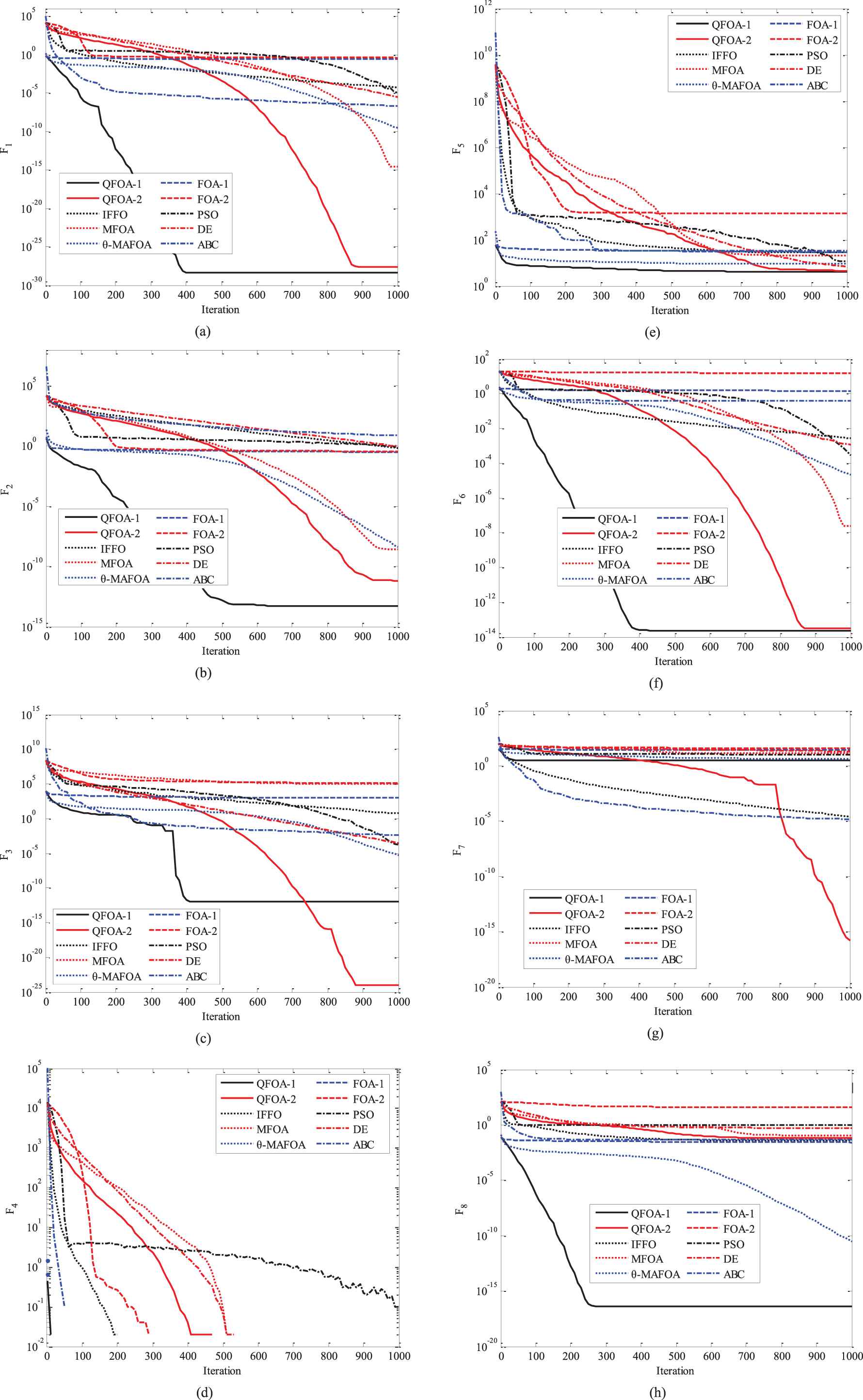
Comparison of convergence curves on benchmark functions with D = 10.
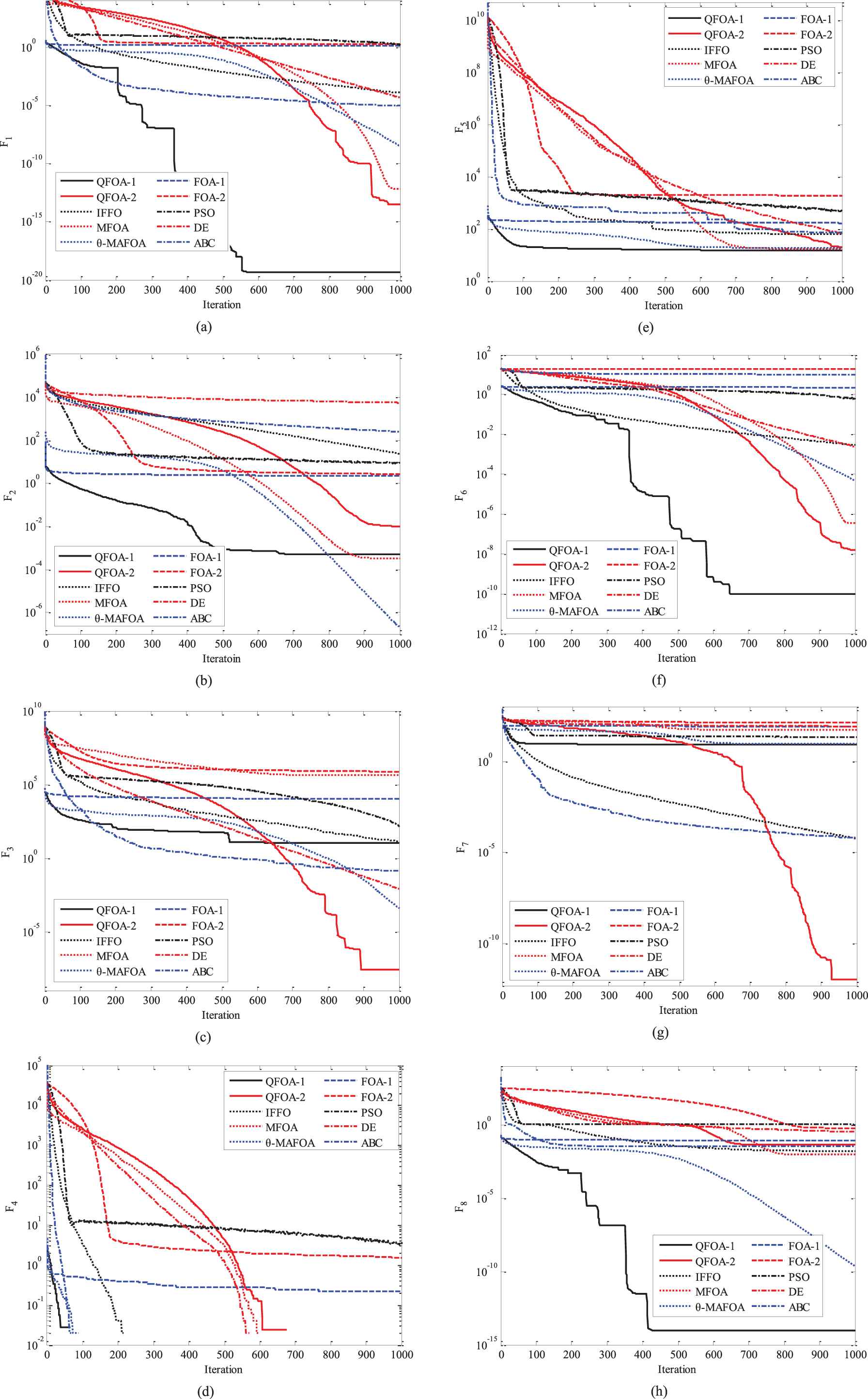
Comparison of convergence curves on benchmark functions with D = 20.
The threat cost f2 penalizes the paths that fly dangerously close to threat sites, which depends on the length and the threat probability of each path segment as follows:
The altitude cost f3 is introduced to make the UAV fly at the low altitude, so that the UAV can benefit from the terrain mask effect. Meanwhile, f3 can penalize the nonfeasible paths that pass through the terrain, as follows:
The lateral maneuvering cost f4 is the sum of those points that do not satisfy the turning constraint as follows:
The vertical maneuvering cost f5 is the sum of those points that do not satisfy the slope constraint as follows:
5.2. Path Representation in 3D Environment
The full UAV path is represented by a collection of N discrete waypoints except the given start and target points. Considering each waypoint pk, k = 1, …, N, are determined by three coordinates (xpk, ypk, zpk), the total dimension of the decision variable in a UAV path is 3N. In order to reduce the problem dimension and meanwhile to obtain the smooth path, the B-Spline-based path representation strategy is adopted in this paper to determine these waypoints and then represent the desired UAV path.
Given n+1 control points with the coordinates (x0, y0, z0), …, (xn, yn, zn), the B-Spline curve can be constructed by [31]
Using the B-Spline-based path representation, if the UAV path is represented by the collection of discrete waypoints {p0, p1, …, pN, pN+1} with the coordinates (xpk, ypk, zpk), k = 1, …, N, for each waypoint, then the corresponding control point collection is {w0, w1, …, wn, wn+1} with the coordinates (xci, yci, zci), i = 1, …, n. Both the first waypoint p0and the first control point w0 are the given start point, while both the last waypoint pN+1 and the last control point wn+1are the given target point. The task of the path planner is to generate n control points, and thus, these control points can achieve the B-Spline curve-based path together with the given start and target points.
5.3. Path Planning Using QFOA
In order to obtain the optimal UAV flight path, the B-Spline curve-based path connecting the given start and target points should have the minimum value of cost function. Using the proposed QFOA models to design the UAV path planner, the coordinates of the control points are treated as the food source of fruit fly swarm. The number of control points is n, and then, D = 3n parameters {x1, x2, …, xD} should be determined by the path planner, where (xi, xn+i, x2n+i), i = 1,2,…,n, denotes the 3D coordinates of the i-th control point wi. That is to say, (xci, yci, zci) = (xi, xn+i, x2n+i). These coordinates take values within the limits of the constrained physics 3D space of the mission map. Each candidate path obtained by path planner is evaluated according to the cost function described in (28), which is employed as the smell concentration judgment function for fruit flies. Suppose that the mission space of the UAV flight path is limited in [0,Lmax]×[0,Wmax], and the maximum flight altitude is Hmax. The following section will show how to apply QFOA models to the path planning problem:
Procedure of path planning using QFOA-1
At the t-th iteration of QFOA-1, locations of the i-th fruit fly is represented by (Xi,1,Xi,2,…,Xi,D) and (Yi,1,Yi,2,…,Yi,D), and the judged value of smell concentration (Si,1,Si,2,…,Si,D) corresponds to the control point coordinates (xc1,…,xcn, yc1,…,ycn, zc1,…,zcn). The detailed implemented procedure of QFOA-1 applied to UAV path planning is described in Algorithm 5.
Procedure of path planning using QFOA-2
For the i-th fruit fly at the t-th iteration in the QFOA-2, both the location and the judged value of smell concentration are represented by (xi,1,xi,2,…,xi,D), which are treated as the decision variable of the optimization problem. Therefore, for the QFOA-2-based path planning problem, the location of the fruit fly (xi,1,xi,2,…,xi,D) corresponds to the control point coordinates (xc1,…,xcn, yc1,…,ycn, zc1,…,zcn), and thus can be decoded into a candidate UAV path using the B-Spline curve. The implemented procedure of QFOA-2 applied to UAV path planning is described in Algorithm 6.
Algorithm 5: Procedure of path planning using QFOA-1
/* Mission */
1. Mission information: start and target points (xS,yS)T, (xT,yT)T,
UAV performance parameters,
the number of the control points n..
2. Threat information: threat centres (xthreat j, ythreat j)T,
threat radius Rj.
3. Map information: the mission map range Lmax,Wmax, Hmax.
/* Initialization */
4. Set the generation counter g = 0.
5. Generation counter g = g + 1;
6. Randomly initialize the fruit fly swarm’s location as [Xaxis, Yaxis] and ensure the judged value of smell concentration S is within the search range [0, 1] D.
/* Iterative search */
7. while termination criteria is not satisfied do
8. Generation counter g = g + 1.
9. Calculate the parameter b = b1 logsig(10 (0.5 −g/Gmax)) + b2.
/* Quantum-behaved search using osphresis */
10. for i = 1: Mospdo
11. for j = 1: Ddo
12. Calculate the characteristic length:
Lx,i,j = 2b|Xaxis – Xi,j|, Ly,i,j = 2b|Yaxis – Yi,j|.
13. while 1 do
14. Generate the random direction and distance as follows:
15. if random > 0.5 then
16. Xi,j = Xaxis,j+ 0.5 Lx,i,j ln(1/rx);
17. else
18. Xi,j = Xaxis,j− 0.5 Lx,i,j ln(1/rx).
19. if random > 0.5 then
20. Yi,j = Yaxis,j + 0.5 Ly,i,j ln(1/ry)
21. else
22. Yi,j = Yaxis,j − 0.5 Ly,i,j ln(1/ry).
23. Calculate the judged value of smell concentration:
24. if Si, j≤ 1 then
25. break.
26. end while
27. end for
/* Evaluation */
28. Set (xc0, yc0, zc0)T as the coordinates of the start point.
29. for j = 1: ndo
30. xcj= Si,j× Lmax
31. ycj= Si,n+j× Wmax
32. zcj= Si,2n+j× Hmax
33. end for
34. Set (xcn+1, ycn+1, zcn+1)T as the coordinates of the target point.
35. Generate the B-Spline curve using the control points (xc0, yc0, zc0)T, …, (xcn+1, ycn+1, zcn+1)T.
36. Evaluate smell concentrations (the cost value) according to (27):
Smelli = J(Pathi), Pathi= [(xc0,yc0,zc0)T,…,(xcn+1,ycn+1, zcn+1)T].
37. end for
/* Search using vision */
38. Select the fruit fly that has the best smell concentration:
index = arg max(Smelli).
39. if [Xindex, Yindex] has the better smell than [Xaxis, Yaxis], then
40. Xaxis = Xindex and Yaxis = Yindex.
41. end while
/*Output*/
42. Decode and output the best path for UAV.
Algorithm 6: Procedure of path planning using QFOA-2
1. Mission information: start and target points (xS,yS)T, (xT,yT)T,
UAV performance parameters,
the number of the control points n.
2. Threat information: threat centres (xthreatj,ythreatj)T,
threat radius Rj.
3. Map information: the mission map range Lmax,Wmax, Hmax.
/* Initialization */
4. Set the generation counter g = 0.
5. Set the number of fruit flies as Mosp as well as parameters b1, b2.
6. Randomly initialize xaxis = [xaxis,1, xaxis,2, …, xaxis,D] with [0, 1] D.
/* Iterative search */
7. while termination criteria is not satisfied do
8. Generation counter g = g + 1.
9. Calculate the parameter b = b1 logsig(10 (0.5 −g/Gmax)) + b2.
/* Quantum-behaved search using osphresis */
10. for i = 1: Mospdo
11. for j = 1: D do
12. Calculate the characteristic length:
Lij= 2b|Xaxis,j – Xij|.
13. while 1 do
14. Generate the random direction and distance as follows:
15. if random > 0.5 then
16. Xi,j = Xaxis,j+0.5 Li,jln(1/rx);
17. else
18. Xi,j = Xaxis,j–0.5 Li,jln(1/rx).
19. if random > 0.5 then
20. break
21. end while
22. end for
/* Evaluation */
23. Set (xc0, yc0, zc0)T as the coordinates of the start point.
24. for j = 1: ndo
25. xcj = xi,j× Lmax
26. ycj = xi,n+j× Wmax
27. zcj = xi,2n+j× Hmax
28. end for
29. Set (xcn+1, ycn+1, zcn+1)T as the coordinates of the target point.
30. Generate the B-Spline curve using the control point set (xc0, yc0, zc0)T, …, (xcn+1, ycn+1, zcn+1)T.
31. Evaluate smell concentrations (the cost value) according to (27):
Smelli= J(Pathi), Pathi= [(xc0,yc0,zc0)T,…, (xcn+1,ycn+1,zcn+1)T].
32. end for
/* Search using vision */
33. Select the fruit fly that has the best smell concentration:
index = arg max(Smelli).
34. if [Xindex, Yindex] has the better smell than [Xaxis, Yaxis], then
35. Xaxis = Xindex and Yaxis = Yindex.
36. end while
/*Output*/
37. Decode and output the best path for UAV.
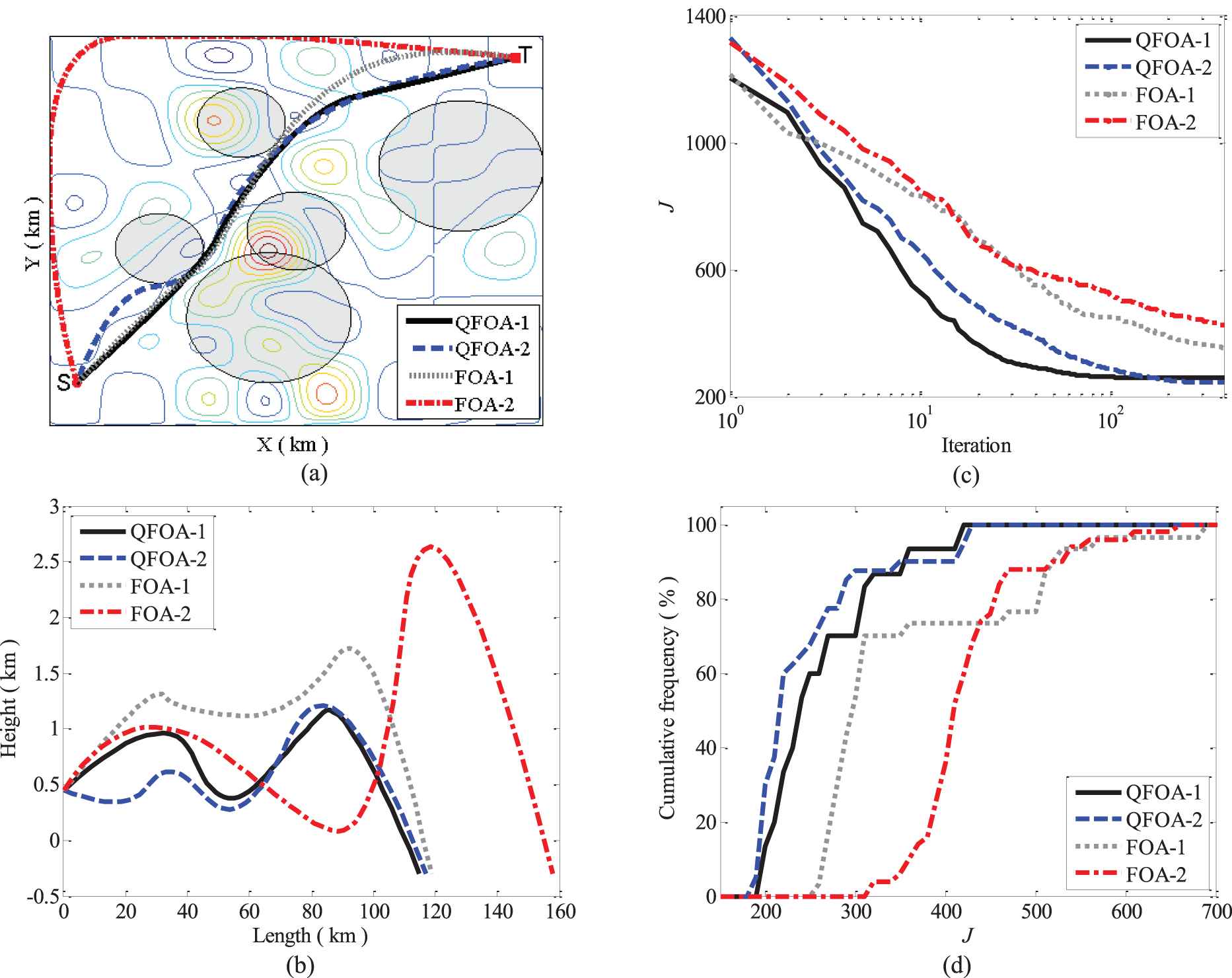
Results comparison on the 1st test scenario, including (a) best paths, (b) flight height of the best paths along the path length, (c) average convergence curves, and (d) cumulative frequency graphs of the cost values.
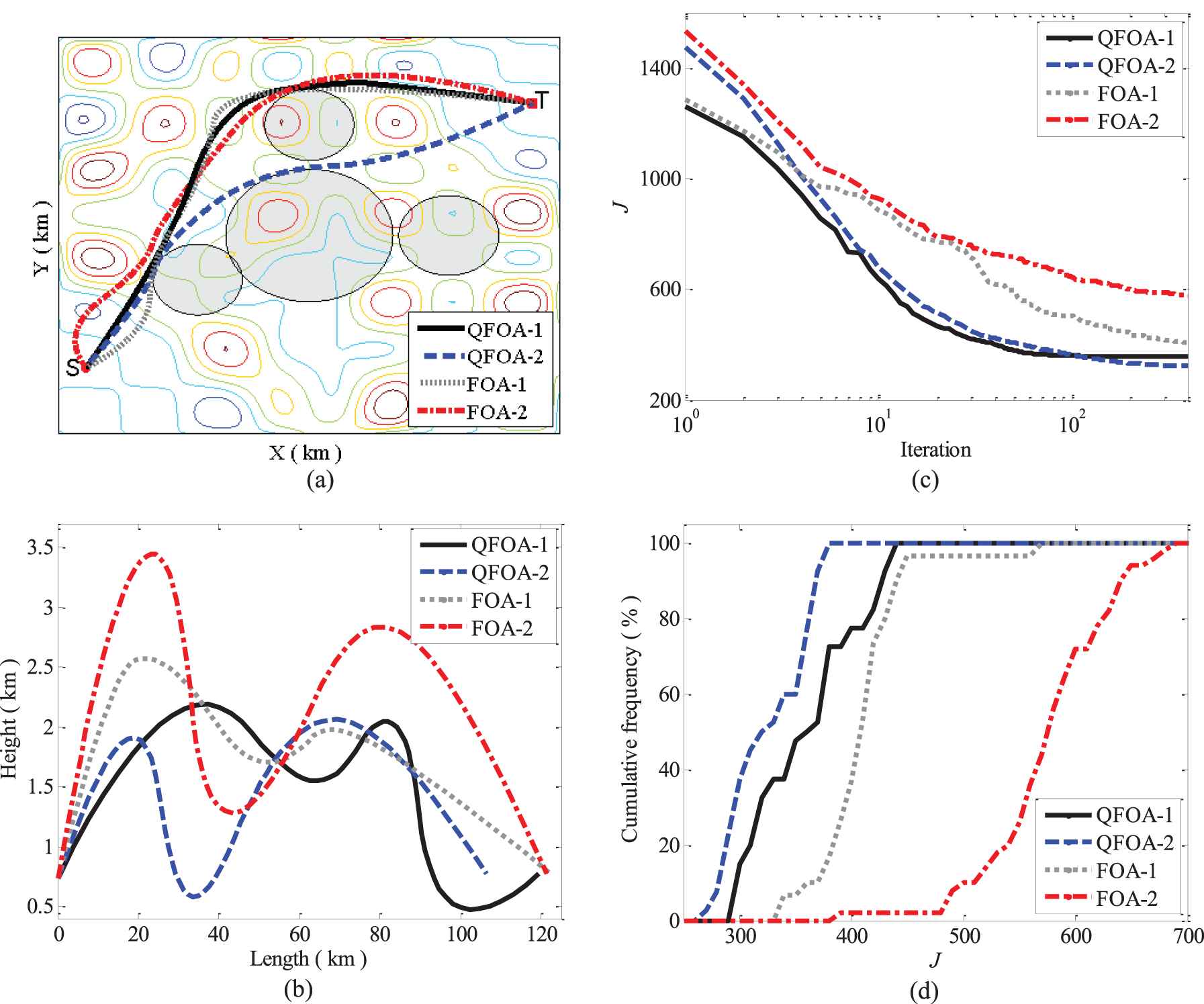
Results comparison on the 2nd test scenario, including (a) best paths, (b) flight height of the best paths along the path length, (c) average convergence curves, and (d) cumulative frequency graphs of the cost values.
6. EXPERIMENT RESULTS
To evaluate our designed QFOA-based path planners, several comparison simulations are carried out. We mainly concern the performance of the proposed QFOA algorithms versus the original standard FOA models, and thus, the QFOA-1, QFOA-2, FOA-1, and FOA-2 are tested under two scenarios in this section. All the tested algorithms are coded using Matlab-2009a on a personal computer. Due to the randomness nature of swarm intelligence algorithms, every tested algorithm is run 50 times independently for each scenario and the statistical results are used for evaluation and comparison. The mission map is a rectangular region with known terrain and threat environments. The number of the B-Spline control points is set as n = 4, which means the dimension of the problem is D = 3n = 12. Other parameters of the UAV are set as the maximum lateral overload nmax= 5, the minimum safety flight altitude Hsafe= 50 m, and the flight velocity V = 200 m/s. To make a fair comparison, the same maximum iteration number is used for all algorithms as the stopping criterion, while the population size is set as Mosp= 40 for all algorithms.
Figures 3 and 4 show the simulation results obtained by QFOA-1, QFOA-2, FOA-1, and FOA-2 on two different scenarios during 50 independent runs. The best UAV paths obtained by the four algorithms on two different scenarios are projected on the xoy contour plane as shown in Figures 3(a) and 4(a), respectively. In the maps, the circle dot “
| Algorithm | f1 | f2 | f3 | f4 | f5 |
|---|---|---|---|---|---|
| QFOA-1 | 114.98 | 0 | 79.24 | 0 | 0 |
| QFOA-2 | 117.15 | 0 | 66.25 | 0 | 0 |
| FOA-1 | 118.89 | 0 | 132.28 | 0 | 0 |
| FOA-2 | 158.45 | 0 | 152.12 | 0 | 0 |
UAV, unmanned aerial vehicle; QFOA, quantum-behaved fruit fly optimization algorithm; FOA, fruit fly optimization algorithm.
Cost values of the best UAV paths obtained by various algorithms on the 1st scenario.
| Algorithm | f1 | f2 | f3 | f4 | f5 |
|---|---|---|---|---|---|
| QFOA-1 | 119.68 | 0 | 177.04 | 0 | 0 |
| QFOA-2 | 106.56 | 0 | 156.19 | 0 | 0 |
| FOA-1 | 122.41 | 0 | 214.62 | 0 | 0 |
| FOA-2 | 121.82 | 0 | 264.83 | 0 | 0 |
UAV, unmanned aerial vehicle; QFOA, quantum-behaved fruit fly optimization algorithm; FOA, fruit fly optimization algorithm.
Cost values of the best UAV paths obtained by various algorithms on the 2nd scenario.
The statistical results of four tested algorithms during 50 runs on two test scenarios are listed in Tables 7 and 8, where the best, median, mean, worst, and standard deviation of the cost value are recorded. The best values of each column are highlighted using boldface. The search ability and stability of a swarm intelligence algorithm can be reflected by the mean cost value and the standard deviation, respectively. Compared these statistical results, it is observed that QFOA-2 obtains the minimum best, mean, median, and worst cost, which indicates QFOA-2 has the most powerful optimization ability in the statistical sense. QFOA-1 also can obtain the smaller value of all statistical results than the original standard FOA models. The convergence curves of the average best cost values are displayed in Figures 3(c) and 4(c). It can be seen that, QFOA models achieve the faster convergence speed and the smaller cost than FOA models. The global convergence performance can be sorted as QFOA-2 > QFOA-1 > FOA-1 > FOA-2.
| Algorithm | Best | Median | Mean | Worst | Std. |
|---|---|---|---|---|---|
| QFOA-1 | 194.22 | 236.36 | 259.84 | 418.38 | 63.70 |
| QFOA-2 | 183.40 | 215.79 | 244.64 | 429.97 | 69.14 |
| FOA-1 | 251.17 | 297.32 | 351.73 | 682.51 | 117.44 |
| FOA-2 | 310.57 | 407.73 | 423.55 | 652.89 | 65.31 |
QFOA, quantum-behaved fruit fly optimization algorithm; FOA, fruit fly optimization algorithm.
Performance comparison on the 1st test scenario.
| Algorithm | Best | Median | Mean | Worst | Std. |
|---|---|---|---|---|---|
| QFOA-1 | 296.72 | 360.20 | 328.21 | 437.77 | 46.92 |
| QFOA-2 | 262.75 | 323.90 | 325.51 | 319.19 | 35.57 |
| FOA-1 | 337.03 | 407.66 | 408.49 | 564.44 | 40.28 |
| FOA-2 | 386.65 | 572.48 | 574.79 | 689.98 | 55.86 |
QFOA, quantum-behaved fruit fly optimization algorithm; FOA, fruit fly optimization algorithm.
Performance comparison on the 2nd test scenario.
Furthermore, in order to study the distribution of the solutions, the cumulative frequency graphs of the minimum cost values during independent runs are listed in Figures 3(d) and 4(d), where the horizontal axis denotes the cost value and vertical axis denotes the cumulative frequency. Define the cumulative frequency as follows:
7. CONCLUSIONS
This paper introduces the quantum theory into FOA model and replaces the osphresis-based search of FOA as the quantum behavior-based searching mechanism, and thus, proposed the QFOA variant. In QFOA models, the Delta potential well is established around the fruit fly swarm location and fruit flies find and move toward the food source following the rules of wave function. Several comparative studies are conducted based on benchmark functions. Results show the proposed QFOA models are superior to the original standard FOA models and other improved FOA variants, as well as several state-of-the-art population-based algorithms, such as DE, PSO, and ABC. The proposed QFOA show the powerful searching abilities, robustness, and global convergence in solving continuous optimization problems.
In addition, the proposed QFOA models are also successfully applied to solve UAV path planning problem and the QFOA-based path planner are designed. The detailed implemented procedures of the path planning are given. Simulation results on two scenarios show that the proposed QFOA can solve this complex optimization problem and achieve much better performance in terms of searching ability, stability, and robustness than the original standard FOA models, which further indicates that the proposed QFOA is the powerful optimization technique.
It is the first work that take advantage of quantum theory to enhance the original FOA. Another contribution of this paper is that the improvement strategy is simultaneously employed to two standard FOA models. In the future work, we will further investigate the performance of the QFOA models and apply the them to the multi-objective optimization problems.
ACKNOWLEDGMENTS
This work is supported by National Natural Science Foundation of China (No. 61703012), Beijing Natural Science Foundation (No. 4182010).
REFERENCES
Cite this article
TY  - JOUR
AU  - Xiangyin Zhang
AU  - Shuang Xia
AU  - Xiuzhi Li
PY  - 2020
DA  - 2020/09/07
TI  - Quantum Behavior-Based Enhanced Fruit Fly Optimization Algorithm with Application to UAV Path Planning
JO  - International Journal of Computational Intelligence Systems
SP  - 1315
EP  - 1331
VL  - 13
IS  - 1
SN  - 1875-6883
UR  - https://doi.org/10.2991/ijcis.d.200825.001
DO  - 10.2991/ijcis.d.200825.001
ID  - Zhang2020
ER  -