
Sequential Prediction of Glycosylated Hemoglobin Based on Long Short-Term Memory with Self-Attention Mechanism
- DOI
- 10.2991/ijcis.d.200915.001How to use a DOI?
- Keywords
- Network; Machine learning; T2DM; Glycosylated hemoglobin; Self-attention mechanism
- Abstract
Type 2 diabetes mellitus (T2DM) has been identified as one of the most challenging chronic diseases to manage. In recent years, the incidence of T2DM has increased, which has seriously endangered people’s health and life quality. Glycosylated hemoglobin (HbA1c) is the gold standard clinical indicator of the progression of T2DM. An accurate prediction of HbA1c levels not only helps medical workers improve the accuracy of clinical decision-making but also helps patients to better understand the clinical progression of T2DM and conduct self-management to achieve the goal of controlling the progression of T2DM. Therefore, we introduced the long short-term memory (LSTM) neural network to predict patients’ HbA1c levels using time sequential data from electronic medical records (EMRs). We added the self-attention mechanism based on the traditional LSTM to capture the long-term interdependence of feature elements and which ensure that the memory was more profound and effective, and used the gradient search technology to minimize the mean square error of the predicted value of the network and the real value. LSTM with the self-attention mechanism performed better than the traditional deep learning sequence prediction method. Our research provides a good reference for the application of deep learning in the field of medical health management.
- Copyright
- © 2020 The Authors. Published by Atlantis Press SARL.
- Open Access
- This is an open access article distributed under the CC BY-NC 4.0 license (http://creativecommons.org/licenses/by-nc/4.0/).
1. INTRODUCTION
Diabetes is a prevalent metabolic disease that reduces life expectancy. The prevalence of diabetes is projected to increase from 4% in 1995 to 4.5% in 2035, and by 2045, the number of people suffering from diabetes is estimated to reach 629 million worldwide, according to the World Health Organization (WHO) [1,2]. Type 2 diabetes mellitus (T2DM), which accounts for more than 90% of diabetes cases, is one of the four priority noncommunicable diseases identified by the WHO [3]. The global prevalence of T2DM is rapidly increasing due to the aging of the population, urbanization, and changes associated with lifestyle [4]. The significant increase in the prevalence of T2DM has imposed high costs on the individual’s health and substantial challenges to national healthcare systems.
T2DM is mainly caused by insulin resistance (insulin secretion is high but the utilization rate is low) and insufficient insulin secretion, which will lead to increased levels of glycosylated hemoglobin (HbA1c). A high HbA1c level not only leads to the deterioration of T2DM but also leads to many fatal health complications, such as kidney failure, blindness, heart disease, etc. [2]. HbA1c is the most valuable index to judge the state of blood sugar control and the progression of T2DM. The detection of HbA1c is simple and easy, and the results are stable and are not affected by meal times and short-term lifestyle changes. Therefore, in the actual clinical decision-making process, medical workers often use HbA1c as the key criterion for assessing the clinical progression of T2DM. They closely monitor the level of HbA1c in patients with T2DM and adjust the treatment plan accordingly to provide the appropriate clinical intervention that will stabilize its levels near the optimal value. In addition, in 2009, the International Expert Committee recommended the use of HbA1c to diagnose T2DM and prediabetes [2]. In 2010, the American Diabetes Association (ADA) endorsed the recommendations of the Expert Committee on the diagnosis of T2DM and recommended HbA1c as the preferred method [5–7]. In 2011, the WHO approved HbA1c as the gold standard for the diagnosis of T2DM [5,6]. In summary, maintaining HbA1c levels is very important for reducing the risk of T2DM and clinical decision-making.
Therefore, many researchers have extensively analyzed HbA1c. For example, Chemlal et al. used patients’ previous HbA1c levels and physical activity as input variables for the risk prediction model for T2DM [8]. Based on this prediction model, Chemlal et al. also implemented a mobile phone application, which predicts and provides feedback on HbA1c levels in patients with T2DM [9]. Torregrosa et al. developed the 3 point-of-care HbA1c analyzer devices for use in physicians’ offices to provide immediate results and reduce inconvenience to the patients [10]. Georga et al. designed a diabetes monitoring and management system through which patients record details about their daily lives, and obtain HbA1c levels and various alarms according to these records [11]. However, most of these studies have focused on the accuracy of HbA1c monitoring or explored the relationship among glycosylated hemoglobin levels and T2DM and its complications. Few studies have examined the future prediction of HbA1c levels and the role of predicted values in the self-management of patients with T2DM. In addition, the results of these studies remain unclear. Therefore, a challenging research issue is to predict the development of trends in HbA1c levels. The HbA1c levels of patients with T2DM changes with time. In practice, HbA1c is regularly checked every three months in patients with T2DM to reflect their blood glucose control in the past 8–12 weeks. This is obviously a typical time sequential prediction problem. In the current deep learning methods of time sequential prediction, the long short-term memory (LSTM) neural network has been proved to have better performance (described in the literature review), so this paper uses LSTM to predict the trend of HbA1c level. In addition, although LSTM has the ability to capture long-term information, the single use of LSTM to capture long-term information is not effective. Because the gap between HbA1c data in patients with T2DM is long. Here, this paper introduces self-attention (SA) mechanism to enhance the ability of LSTM to capture long-term information, so as to more accurately apply it to the prediction of HbA1c data. In the present study, we aim to accurately predict the future HbA1c levels based only on previous HbA1c levels recorded for patients to ensure that if patients will be able to receive data about a future HbA1c level in advance and only rely on a simple indicator, namely HbA1c records, they will be able to simply and easily manage their T2DM.
The structure of this article is described below. In Section 2, we briefly review the common models that have been applied to predict sequential events. In Section 3, we clarify data acquisition and processing methods. In Section 4, we provide detailed descriptions of the principles and frameworks of the long short-term memory with self-attention mechanism (SA-LSTM) model. Section 5 describes the experimental process and analyzes the results, Section 6 discusses the experimental results, and Section 7 contains the conclusions.
2. LITERRATURE REVIEW
The future development of T2DM mainly depends on the patients’ conditions and interventions received over a long period, and the prediction of T2DM based on the HbA1c level is a sequential predictive event. Additionally, the data of HbA1c levels obtained from EMR used in this paper are time sequential and have the characteristics of continuous and irregular intervals. Therefore, we should use time sequential methods to construct the prediction model, which is consistent with the dynamic development of T2DM. The existing time sequential prediction models in the field of medical health management are described below.
Many researchers have used time discretization data to construct time sequential prediction models, among which the classical models are continuous-time Markov chain models and time Bayesian networks. Bueno et al. used hidden Markov models that are able to cope with uncertainty and sequential phenomena to propose a probabilistic framework for predicting disease dynamics guided by latent states [12]. Nazari et al. suggested that the implementation of a Markov model with a continuous-time process would yield better results for modeling diabetes. By considering the time intervals between the changes in the disease states, the model would provide a more comprehensive perspective of the processes involved in the disease [13]. However, the time interval of each admission is irregular, leading to the irregular intervals of recorded data. In addition, the information recorded at each admission includes continuous data, such as biochemical parameters, discrete variables, and medication data. Continuous-time Markov chain models are often unable to adequately address these complex data. Therefore, Bueno et al. used a dynamic Bayesian network (DBN) model to capture changes in the patient status distribution and explore potential pathophysiological changes over time [14]. Liu et al. noted that typical time Bayesian networks are divided into dynamic Bayesian networks with an assumption of discrete time and continuous-time Bayesian networks with an assumption of continuous time when studying disease processes and compared the advantages of the two networks in different data distributions [15]. Although this approach is advantageous for analyzing complex medical data, its power has yet to be confirmed, and it further assumes that discrete states are inefficient [3,16].
As new application of deep learning methods in the medical health management field are becoming increasingly successful, particularly in medical image and sound data, deep learning methods have attracted increasing attention, among which LSTM is the most advanced method [17,18]. Reddy and Delen used a recurrent neural network (RNN)-LSTM method to predict hospital readmissions for patients with lupus [19]. Tsiouris et al. introduced LSTM networks to predict epileptic seizures based on EEG signals and verified that the proposed LSTM-based methodology delivers a significant increase in seizure prediction performance compared to both traditional machine learning techniques and convolutional neural networks [20]. Swapna et al. employed deep learning networks with a convolutional neural network—LSTM to automatically detect the abnormality of heart rate variability signals [17]. Most of these studies used LSTM to generate relevant predictions with time sequential EMR data, which are critical for understanding and slowing disease progression. LSTM has a strong adaptability in time sequential data analysis and performs better in sequence learning than other traditional predicting methods, such as RNNs, support vector machines, hidden Markov models, etc.
However, for long-term interdependence, LSTM must incorporate several time steps of information accumulation to link the data. A longer time results in a lower the effectiveness of capturing information is [21]. Therefore, we introduce the SA mechanism, an efficient deep learning method, to address the shortcomings of LSTM. The SA mechanism ensures that the memory of LSTM is more profound and effective by adequately capturing long-term information interdependence to improve the accuracy of the prediction. In fact, the SA mechanism was first applied in image processing field. With the continuous development of the SA mechanism, it has become a research hotspot in neural networks and has been used in combination with other deep learning methods in different fields and has shown good performance. Wu et al. integrated the SA mechanism into a convolutional neural network to improve image fidelity for accelerated magnetic resonance image acquisition [22]. Vuddagiri et al. constructed deep neural networks with attention architectures (DNN-WA) to develop automatic language identification systems, and the proposed model performed better in terms of an equal error rate [23]. Cinar et al. extended the attention mechanism into RNNs for time sequential forecasting with missing values [24]. However, the SA mechanism is rarely used in the medical health management field or in combination with LSTM. The SA mechanism better solves the problem of long-term interdependence of LSTM in theory. The integration of LSTM and the SA mechanism in the medical health management field requires further study.
In summary, we construct the SA-LSTM model to predict patients’ HbA1c levels using time sequential data in this paper. We compare this improved model with the traditional LSTM and random forest (RF) models to study the effectiveness of the integrated SA-LSTM model in time sequential predictions.
3. DATA PREPROCESSING
3.1. Data Source
We obtained 6009 records from the electronic medical records (EMRs) provided by The Anhui Provincial Hospital of Traditional Chinese Medicine, and 3885 effective patient records were retrieved. These EMRs are digital versions of patients’ health information documented from 2012 to 2018, which store basic personal information (age, sex, marital status, etc.), laboratory test results (glycosylated hemoglobin, fasting blood sugar, fasting C-peptide, etc.), diagnostic information (admission time, discharge time, ICD-10, etc.), and drug information (drug name, dosage, route of drugs, etc.). Every patient has a complete EMR each time he or she is hospitalized.
3.2. Data Processing
Because patients stay in hospital for a long time and medical workers closely monitor patients’ glycosylated hemoglobin levels during hospitalization, every patient in the hospital has more than one glycosylated hemoglobin value in the EMR. We screened patients who had been hospitalized five or more times, because fewer hospitalizations do not reflect the trend of glycosylated hemoglobin levels and are not meaningful for predictions and may even reduce the accuracy of prediction. Then, we selected the glycosylated hemoglobin values and the time of each test during each patient’s hospitalization from each complete EMR. The time of hospitalization for each patient varied according to the severity of T2DM, but was usually approximately 14.56 days. In addition, the intervals between hospitalizations were irregular, and thus we used sequential data with irregular intervals. The basic statistics of the effective data are shown in Table 1. We sequentially arranged the data according to the time of each patient’s detection of glycosylated hemoglobin level. Each glycosylated hemoglobin value is reported as a percentage. Detailed data structures are shown in Table A1 of the Appendix.
| ITEM | Statistical Results |
|---|---|
| Total number of patients | 3885 |
| Average number of HbA1c records per hospitalization | 23 |
| Average duration per hospitalization | 14.56 days |
| Average interval between hospitalizations | 184.52 days |
| Max HbA1c level | 16.8% |
| Min HbA1c level | 4.1% |
The basic statistics of data.
4. MODEL
4.1. Self-ASA Mechanism
The attention mechanism was first proposed in the field of visual images. In recent years, the attention mechanism has been widely used in natural language processing based on deep learning methods and achieved good results. Its core idea is to draw lessons from the fact that the human brain will focus on a particular place at a particular time and allocate less attention to unimportant information. The SA mechanism is a special variant of the attention mechanism. More specifically, the attention mechanism occurs between an encoder and decoder, or between input and output information. The SA mechanism occurs within the information sequence and captures the connections between the distant information, which is also called internal attention.
The principle of the SA mechanism is understood from the perspective of key value query. As shown in Figure 1, the key value query has three basic elements: Query, Key, and Value. Supposing we have n key vectors
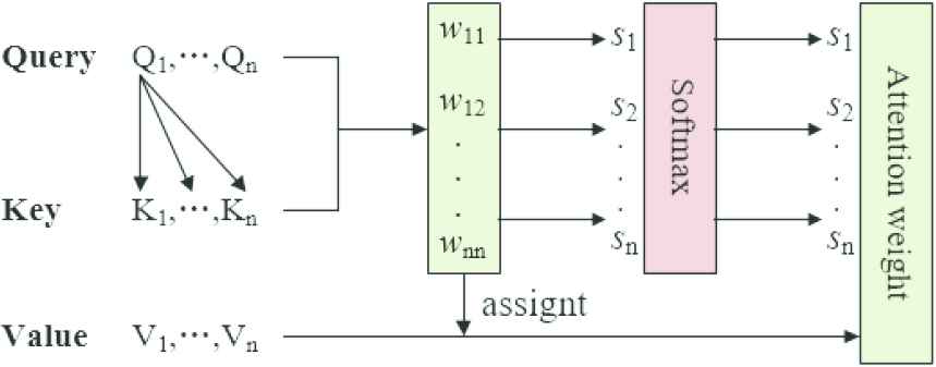
The principle diagram of the self-attention mechanism.
The computational steps of the SA mechanism are described below.
Calculate the similarity of each Query and Key to obtain
By introducing a similar softmax function to normalize the weights, the weights of important elements become more prominent. The calculation is shown in formula 4.
The final attention value is obtained by the weighted summation of
4.2. Long Short-Term Memory
LSTM is a variant of the RNNs proposed by Hochreiter and Schmidhuber in 1997 [25]. LSTM is suitable for learning from experience and predicting time sequential problems, which is also a difference from other neural network models. The key feature of LSTM to solve time sequential problems is the cell state. LSTM adds and deletes information from the cell state. We must use an information gate, namely, the forgetting gate, input gate and output gate, to achieve this goal. LSTM forgets, retains, and outputs historical information through gate selectivity [26]. The specific structure of LSTM is shown in Figure 2.

The specific structure of long short-term memory (LSTM).
In Figure 2, h denotes the output, x denotes the input, tanh denotes the hyperbolic tangent function, σ denotes the sigmoid function, and A denotes a hidden layer node. As shown in the figure, the gates in LSTM are controlled or activated by a sigmoid function. The output value of the sigmoid function ranges from 0 to 1, which determines how much information is passed through the gate. If the sigmoid function output is 0, the information is not transmitted. If the output is 1, all information is transmitted.
The information processing steps of LSTM are described below.
A decision is made about which historical information must flow into the cell through the sigmoid network layer of the forgetting gate. It is expressed using the following formula:
whereThe new information that must be updated through the input gate is determined. A sigmoid network layer is used to determine the weight of the information that must be updated and a tanh layer is used to calculate the alternative content for updating the current cell. It is expressed using the following formulas:
whereThe cell state is updated by multiplying the output value of the forgetting gate by the old cell state
The information that flows into the next cell from the current cell through the output gate is determined. Similarly, a sigmoid network layer is used to calculate the weight of the output information and then a tanh layer is used to process the information after the current cell is updated. The final output of the current cell is obtained by multiplying the two using the following formula:
where
4.3. Integrated SA-LSTM Model
Based on the introduction to LSTM provided above, it has a good memory of previous information and is a very suitable method for time sequential prediction research. However, as mentioned above, LSTM has a long-term interdependence problem, namely, LSTM calculates hidden states and outputs in a stepwise manner for input sequences, but is unable to easily capture the connections between long-term distant data. It may require more time steps to react. For patients with T2DM, the HbA1c level measured in the hospital undergoes dynamic changes over time. These sequential data are limited and intrinsically correlated, but not an isolated set of points. Therefore, the prediction results obtained using LSTM alone may not be ideal. In this paper, we introduced the SA mechanism into the traditional LSTM method to improve the accuracy and applicability of the prediction. The SA mechanism focuses on sequential information at different times and fully adopts all the contents in front of the sequence to better solve the problem of long-term interdependence [27]. The introduction of the SA mechanism enables the model to store the important intermediate information of the current moment for a subsequent time, which better expands the expressive ability of the neural network and enhances the long-distance interdependence effect.
As shown in Figure 3, the integrated SA-LSTM model consists of four modules: input layer, LSTM layer, SA mechanism layer, and output layer.
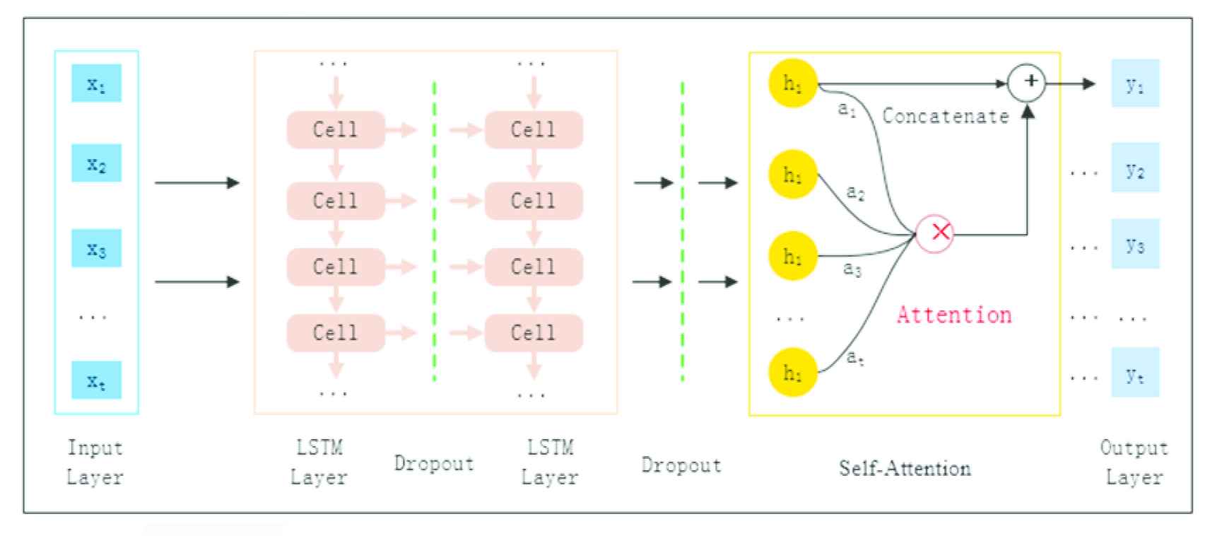
The structure of the integrated self-attention long short-term memory (SA-LSTM) model.
Input layer: Introduce glycosylated hemoglobin time sequential data from patients with T2DM. The input layer requires three dimensions, namely, sample capacity (batch size), time series (time step), data content (input data). Combined with this experiment, the sample size is the total number of patients with T2DM. Each patient enters the input layer as a sample. Each patient contains a number of sequential glycosylated hemoglobin values to form a time series. The specific glycosylated hemoglobin values in each time series are the data content [26]. See Table A1 of the Appendix for specific sample input values.
LSTM layer: There are two LSTM layers. The first LSTM layer includes 35 memory cells and the second LSTM layer, includes 30 memory cells. We introduce Dropout, which is a way to overcome network over-fitting, and adjust the learning ability of the neural network model and learn more robust features adaptively. The dropout rates are set to 0.5.
SA mechanism layer: The SA layer uses a multiple linear regression analysis to sense the effect of input data on the predicted value and calculates the weighted value of each feature that affects the predicted value. The SA mechanism achieves a linear combination of all hidden states in LSTM with different weights. Set the input matrix as
Then
whereOutput layer: We use regularization to add penalty items to the coefficients trained by the network to reduce the test error. The penalty items punish those coefficients that are too large and increase the coefficients that are too low to prevent the model from over-fitting and obtain the final output. In this experiment, the output layer has only one dimension, that is, the predicted value of glycosylated hemoglobin.
The flow-process of the proposed model is shown in Figure 4. First, we collected the HbA1c test value and test time of T2DM patients. Then, we normalize the preprocessed sequential HbA1c data as the original input data with the formula 12. We train the proposed model with 30% samples to adjust and optimize the parameters. Besides, the feature information of input data is extracted by the LSTM layer and a deep information structure feature is obtained. The SA mechanism operates on the output of LSTM layer using scaled point product attention to learn the structural characteristics of time sequential data and capture long-term interdependence. Finally, we added a regularization term (expressed as the formula 13) to the cost function to reduce the influence of disturbance and noise in training data and obtain the prediction results.
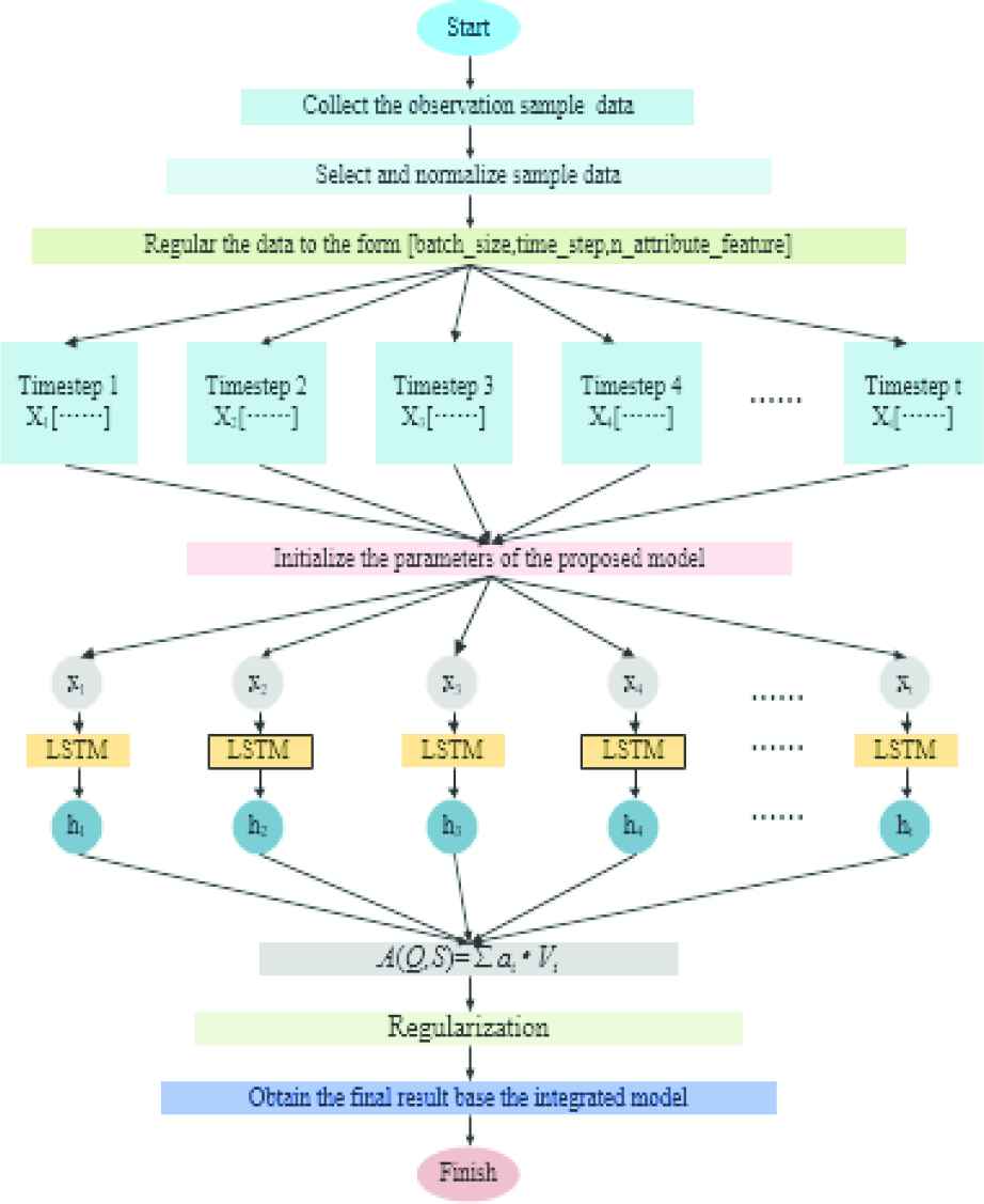
The flow-process diagram of the integrated self-attention long short-term memory (SA-LSTM) model.
5. EXPERIMENT AND RESULT
5.1. Experiment
5.1.1. Experimental setting
We extracted HbA1c data and test times from the EMR of patients with T2DM to form datasets. We considered using previous data records of patients to predict the last value. We used previously recorded data for each patient as characteristics, and the last data point as the prediction label. Patients whose sample size was less than 5 were excluded. Finally, we divided these processed data into 7:3 parts: 70% of the datasets were used to train the model and 30% of the datasets were used for testing. We used the above data to train the integrated SA-LSTM model proposed in this paper and obtain the prediction results. The accuracy of the prediction results obtained using the integrated SA-LSTM model must be verified; therefore, we chose the RF and the traditional LSTM models, which have performed well in the time sequential prediction task, for comparison to prove the superiority of the model.
RF, a machine learning method, has been widely used in medicine, psychology, energy, and other fields in recent years because of its fast training speed, strong generalization ability, and ability to process high-dimensional data. A large number of studies using the RF model have revealed better performance in time sequential prediction tasks than most machine learning methods [28]. For example, Zhao et al. used a RF regression model to predict outcomes of chronic kidney disease from EMR data and noted that the RF algorithm showed higher stability and robustness with varying training parameters and better success rates and ROC analysis results [29]. Galiano et al. confirmed that RF outperformed an Artificial Neural Network, Regression Tree, and Support Vector Machine for modeling mineral prospectivity [30]. Daghistani et al. evaluated the abilities of an Artificial Neural Network, Support Vector Machine, Bayesian Network, and RF to predict the in-hospital length of stay (LOS) [31]. The RF model provided more accurate LOS predictions for patients with heart disease. LSTM is the most advanced deep learning method, as we have already specified in the second part of the literature review. Here, we compared the integrated SA-LSTM model proposed in this paper with LSTM and RF in the same data environment.
RF: Because the prediction target is based on continuous-time sequential data, we adopted the regression strategy in the method.
LSTM: Although LSTM adds threshold control based on RNN, almost all papers using LSTM have different structure and parameter settings for the LSTM model. In this experiment, the input dimension of LSTM model is three, data passes through two hidden layers, and the size of each hidden layer is four. The model has been trained and iterated 6000 times.
The integrated SA-LSTM model: The input of the network is the same as LSTM, except that the SA layer is added to the internal structure. LSTM is used to extract time sequential information and the SA mechanism is used to differentiate the importance of sequential information. The model has been trained and iterated 3000 times.
5.1.2. Parameter settings
The main parameters and their values in this experiment are shown in Table 2. In this paper, we find the appropriate range of learning rate based on continuous iterative training, and we finally choose 2 as the learning rate. Because there are 84000 lines of data and 3000 times of training, the batch size is 28 (84000/3000). In practice, three or two layers of neural network are generally selected. Deeper neural network will not only lead to over-fitting, but also increase the difficulty of experimental calculation. In this paper, we find that the performance of two-layer neural network is better than that of three-layer neural network. So we choose two hidden layer units. When the dropout rate is equal to 0.5, the effect is the best, because dropout randomly generates the most network structures at this time.
| Parameters | Parameter Description | Value |
|---|---|---|
| R | Learning rate | 2 |
| Batch_size | Data batch processing | 28 |
| Hidden_units | Number of hidden layer unit | 2 |
| Dropout | Neuron discarding rate | 0.5 |
Main parameters and their values in the experiment.
5.1.3. Evaluation index
In this paper, we use mean square error (MSA), root mean square error (RMSE), mean absolute error (MAE), and mean absolute percentage error (MAPE), which are often used as criteria to measure the predicted results of deep learning models, to evaluate the experimental results. MSE is the sum average of the square of the difference between the real value and the predicted value. RMSE is used to measure the deviation between the real value and the predicted value. MAE, also known as mean absolute deviation, better reflects the actual situation of the predicted value error and avoids the problem of mutual cancellation of errors. MAPE is used to evaluate the prediction effect of different models using the same data. The related calculations are shown in formulas (14–17).
5.1.4. Model training
In this paper, a gradient descent algorithm is used for model training and an MSE loss function is used for the loss function. The goal of the model is to minimize the difference between the predicted output value of HbA1c and the real value in the training sample. The calculation of the difference is shown in formula (15).
5.2. Results
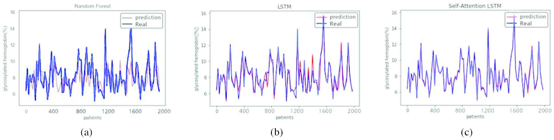
We used RF and LSTM, two commonly used time sequential prediction models, to conduct comparative experiments with the integrated SA-LSTM model. All three models were trained and tested on the same dataset to avoid interference from other factors. The results are shown in the figures below, where the abscissa represents the number of samples in this experiment and the ordinate represents the value of HbA1c. Figure 5 shows the degree of fit of the predicted values and real values from the three models at 1000 sample sizes. Figure 6 shows the degree of fit of the predicted values and real values from the three models at 2000 sample sizes. Figure 7 shows the degree of fit of predicted values and real values from the three models at 3000 sample sizes.
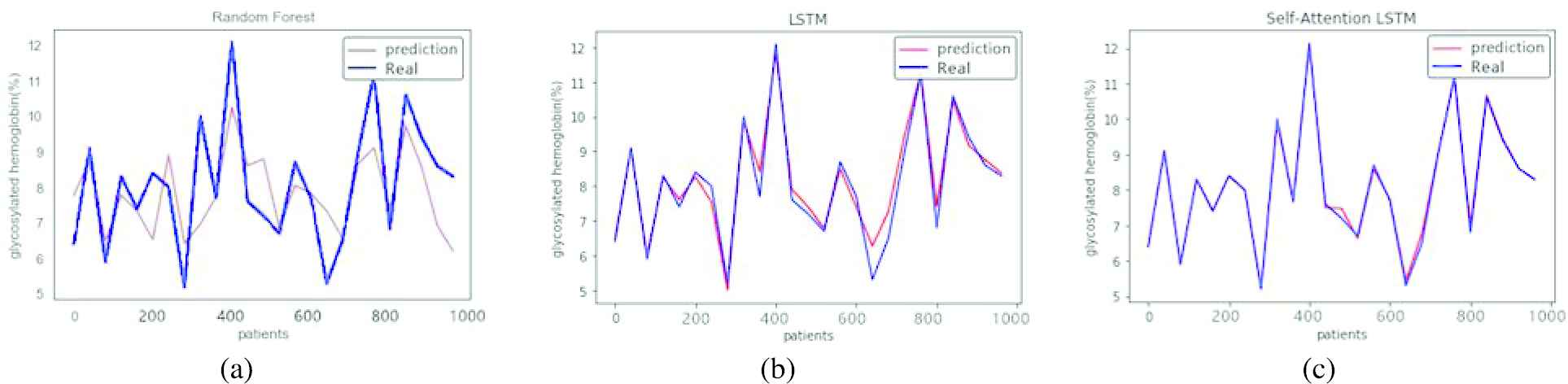
Predicted values from the three models at 1000 sample sizes. (a) The degree of fit of the predicted values and real values obtained by random forest RF. (b) The degree of fit of the predicted values and real values obtained by long short-term memory LSTM. (c) The degree of fit of the predicted values and real values obtained by the integrated self-attention long short-term memory SA-LSTM model.
Predicted values from the three models at 2000 sample sizes. (a) The degree of fit of the predicted values and real values obtained by random forest RF. (b) The degree of fit of the predicted values and real values obtained by long short-term memory LSTM. (c) The degree of fit of the predicted values and real values obtained by the integrated self-attention long short-term memory SA-LSTM model.
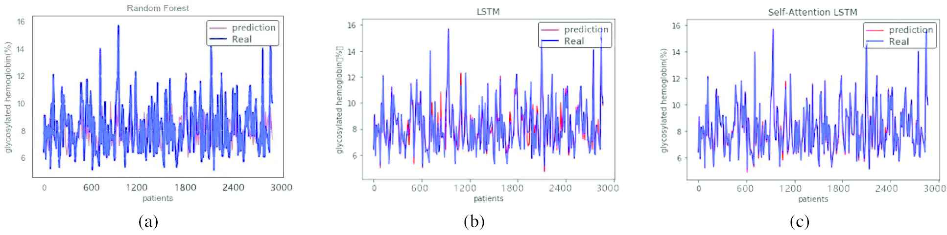
Predicted values from the three models at 3000 sample sizes. (a) The degree of fit of the predicted values and real values obtained by random forest RF. (b) The degree of fit of the predicted values and real values obtained by long short-term memory LSTM. (c) The degree of fit of the predicted values and real values obtained by the integrated self-attention long short-term memory SA-LSTM model.
As shown in Figure 5, when the sample size is 1000, the predicted HbA1c values obtained using LSTM and the integrated SA-LSTM model were very similar to the real values, and the results obtained using RF were not ideal compared with the other two models. As shown in Figure 6, when the sample size is 2000, LSTM was more accurate than the RF prediction, and the performance of the integrated SA-LSTM model was obviously better than RF and LSTM. In Figure 7, when the sample size is 3000, the integrated SA-LSTM model provided the best prediction of the HbA1c levels, and an almost perfect match was observed between the predicted values and real values. In particular, the prediction accuracy of the integrated SA-LSTM model was higher with larger sample sizes.
The evaluation results of the integrated SA-LSTM model proposed in this paper, RF and LSTM on 3000 sample datasets are shown in Table 3.
| Model | MSE | RMSE | MAE | MAPE |
|---|---|---|---|---|
| RF | 2.6750 | 1.6355 | 1.2091 | 13.8962 |
| LSTM | 0.3582 | 0.5985 | 0.4126 | 5.2726 |
| SA-LSTM | 0.0230 | 0.1516 | 0.1037 | 1.3764 |
Evaluation results using different criteria.
As shown in the table, when predicting HbA1c levels, the MSE, RMSE, MAE and MAPE of the integrated SA-LSTM model increased by 99.14%, 90.73%, 91.42% and 90.09%, respectively, compared with the RF model. The integrated SA-LSTM model improved the MSE, RMSE, MAE and MAPE by 93.28%, 74.67%, 74.87% and 73.90%, respectively, compared with LSTM. The integrated SA-LSTM model was significantly better than the RF model and showed better predictive performance than LSTM. This finding confirms the feasibility and superiority of the integrated SA-LSTM model, and the introduction of SA mechanism plays an important role in optimization of traditional sequential prediction methods. The SA mechanism solves the problem of long-term interdependence in deep learning methods such as LSTM and improves the accuracy of the time sequential prediction model by increasing the long-distance interdependence of feature elements.
6. DISCUSSION
We have compared the performance of the integrated SA-LSTM model with RF and traditional LSTM models. The performance was evaluated by calculating the MSE, RMSE, MAE, and MAPE. As shown in Table 3, the integrated SA-LSTM model achieved a higher prediction performance than the RF and traditional LSTM models, which are competitive deep learning methods used to generate time sequential predictions. This result may be easily explained.
In this paper, we use regression strategy for the compared RF method. This method refers to the analysis and prediction of samples by building a combination model of multiple decision trees. Each decision tree model will have a prediction value. The regression method will calculate the average value of the prediction value of each tree to obtain the final prediction value. This approach often results in a failure of the RF model to make predictions beyond the range of data in the training set during the regression. When noisy data are present in the dataset, this method is likely to over-fit to reduce the accuracy of the prediction generated by the model. However, the HbA1c levels from patients with T2DM used in this paper will inevitably produce some noisy data due to the long interval and low frequency of data collection. Therefore, the use of RF to predict the HbA1c level in this experiment is not ideal.
LSTM is powerful in analyzing sequential problems because it is able to control the proportion of historical information being remembered through the gate structure and constantly updates the instant information in the new state. In addition, LSTM has a large number of nonlinear transport layers, and its feature expression is more detailed than traditional models; therefore, it can be used in complex modeling environments. When a sufficient number of training samples is available, the LSTM model completely mines the information contained in the dataset without being disturbed by noisy data. However, as mentioned above, LSTM inevitably has the problem of long-term interdependence, namely, when the time at which sequential data were collected is prolonged, the initial information will disappear when time accumulates to a certain value. However, the time interval between patients’ visits to the hospital to detect HbA1c levels is very long. Using the data collected in this paper as an example, the average time interval for detecting HbA1c levels was 184.52 days and the shortest time interval was 28.44 days. Therefore, LSTM is unable to save and transmit information for a long time in this experiment, which reduces the accuracy of the prediction.
Based on these findings, we proposed the integrated SA-LSTM model, which improves the accuracy of the prediction from three aspects by introducing SA mechanism. (i) Capturing long-term interdependence: Attention is computed for the data of time nodes in the SA mechanism; thus, regardless of the distance between the nodes, the maximum path length is only 1, which captures long-term dependencies and improves long-term memory ability. Therefore, the integrated SA-LSTM model improved the MSE, RMSE, MAE, and MAPE by 93.28%, 74.67%, 74.87%, and 73.90%, respectively, compared with LSTM. (ii) Learning the interdependence in the process of sequence transformation: The SA mechanism effectively solves the problem of information loss in different time steps by learning the interdependence relationship in the process of sequential data transformation to improve the accuracy of the prediction generated by the model. However, the RF model is unable to capture the internal relationships of the information and ignores the relationships in the process of sequence transformation. Therefore, the prediction accuracy of the RF model is much lower than the integrated SA-LSTM model for the different measurement indicators, and is reduced by 99.14%, 90.73%, 91.42%, and 90.09%, respectively. (iii) Improving the output quality of the dynamic structure of the model. As shown in Figures 4–6, the degree of fit between the predicted values and the real values obtained from the integrated SA-LSTM model is higher than the RF and the traditional LSTM models, because both the RF and the traditional LSTM models inevitably lose some of the historical information in the prediction process and are unable to distinguish the importance of the retained information. However, the introduction of the SA mechanism enables the model to dynamically acquire some information that requires attention at different times. Therefore, the model more effectively obtains useful information between input data and output data, and then generates a more reasonable output.
7. CONCLUSION
In recent years, the risk of T2DM has consistently increased, which seriously affects people’s quality of life and health. A reduction in the risk of T2DM not only relies on the clinical treatment but also on another very important role, prognosis self-management. The rational implementation of prognosis self-management activities requires patients to have a clear and correct understanding of their current and future situations. Therefore, this paper proposes the integrated SA-LSTM model to predict HbA1c levels, a gold standard indicator that adequately measures the progression of T2DM. The integrated SA-LSTM model introduces the SA mechanism into the hidden layer of the traditional LSTM model, which addresses the limitation of the long-term interdependence of LSTM by utilizing the ability of the SA mechanism to connect distant information. The integrated SA-LSTM model performed better than the RF and traditional LSTM models in predicting HbA1c levels in patients with T2DM.
This paper has three main contributions: (i) SA mechanism solves a persistent problem of LSTM model well and the integrated SA-LSTM model can more accurately predict the sequential trend of HbA1c in patients with T2DM. It provides a good reference for the improvement of deep learning methods in the field of medical and health management. (ii) HbA1c is a key clinical indicator for evaluating the progression of T2DM. Grasping the sequential trend of HbA1c accurately will help patients to better understand their future illness state and adopt a reasonable self-management strategy to reduce the risk of T2DM. (iii) Accurate prediction of HbA1clevel can help medical workers to judge the progression and condition of patients with T2DM, so as to improve the scientific diagnosis and decision-making of medical workers. This is an important basis for rational utilization and optimal allocation of social medical resources. Of course, some limitations in this paper must be acknowledged. First, the prediction of HbA1c levels provides a prognostic self-management strategy for patients only from the perspective of clinical testing information. The prediction model also must incorporate patients’ individual signs and social networks, which have been proven to affect the risk of T2DM, to help patients manage T2DM more comprehensively. Second, most of the patients included in this study were hospitalized five times or more, and the average interval was 184.52 days. If a greater number of hospitalizations occurred at a shorter interval, the sequential data for the HbA1c level would be more conducive to increasing the specific accuracy of the prediction. These shortcomings provide a direction for our future research, such as methods to incorporate patients’ individual characteristics, which are discontinuous and nonsequential data, into the time sequential prediction. Furthermore, we plan to examine whether these features are realized by modifying the initial state of time sequential prediction methods or by acquiring the external input actively at any time step according to the specific event. Moreover, with the emergence of new models of neural networks, the appropriate design of the SA mechanism to better integrate with the new models is also a hot topic to study [16].
In summary, this paper proposed the integrated SA-LSTM model to predict HbA1c levels, which has guiding significance for improving the health management level and reducing the future risk of T2DM. The study further verifies the feasibility of applying deep learning in the field of medical and health management. In the future, we will further study the existing methods and models to improve the adaptability and superiority of deep learning in the field of medical and health management.
CONFLICTS OF INTEREST
The authors declare no conflicts of interest.
AUTHORS’ CONTRIBUTIONS
Xiaojia Wang and Wenqing Gong contributed to the conception of the study; Xiaojia Wang and Keyu Zhu performed the experiment; Yuxiang Guan and Lushi Yao contributed significantly to analysis and manuscript preparation; Wenqing Gong performed the data analyses and wrote the manuscript; Shanshan Zhang and Weiqun Xu helped perform the analysis with constructive discussions.
ACKNOWLEDGMENTS
This work was supported by a grant from the Key Disease of Diabetes Mellitus Study Center at the National Chinese Medicine Clinical Research Base, the China Scholarship Council, the National Natural Science Foundation of China Grant No. 61876055,71101041, Philosophy and Social Science Cultivation Program of Hefei University of Technology Projects Grant No. JS2019HGXJ0040, JS2019HGXJ0038, National Steering Committee for Graduate Education of Chinese Medicine and Traditional Chinese Medicine Grant No. 20190723-FJ-B39.
APPENDIX
| Row ID | Patient Code | Inhospital ID | HbA1c | Unit |
|---|---|---|---|---|
| 1 | 78452 | 121379 | 8 | % |
| 2 | 78452 | 122476 | 7.5 | % |
| 3 | 78452 | 122950 | 7.8 | % |
| 4 | 78452 | 124004 | 8 | % |
| 5 | 78464 | 120360 | 7.5 | % |
| 6 | 78464 | 118300 | 6.9 | % |
| 7 | 78464 | 119321 | 10.2 | % |
| 8 | 78468 | 117412 | 8.9 | % |
| 9 | 78468 | 117758 | 8.7 | % |
| 10 | 78468 | 117571 | 7.4 | % |
| 11 | 78468 | 117952 | 6.6 | % |
| 12 | 78469 | 117553 | 5.3 | % |
| 13 | 78469 | 117389 | 8 | % |
| 14 | 78477 | 121463 | 7.5 | % |
| 15 | 78477 | 123065 | 7.4 | % |
| 16 | 78477 | 118913 | 6.5 | % |
| 17 | 78477 | 118330 | 8.9 | % |
| 18 | 78481 | 117382 | 9.3 | % |
| 19 | 78482 | 117568 | 9.6 | % |
| 20 | 78482 | 117403 | 8.9 | % |
| 21 | 78486 | 117651 | 5.8 | % |
| 22 | 78488 | 122945 | 6.8 | % |
| 23 | 78488 | 122754 | 6.5 | % |
| 24 | 78491 | 117422 | 6.3 | % |
| 25 | 78491 | 117453 | 5.7 | % |
| 26 | 78494 | 121499 | 6 | % |
| 27 | 78494 | 119248 | 7.5 | % |
| 28 | 78498 | 120296 | 6.5 | % |
| 29 | 78498 | 120101 | 6.3 | % |
| 30 | 78498 | 119963 | 7.2 | % |
| 31 | 78498 | 119504 | 7.1 | % |
| 32 | 78498 | 121439 | 6.2 | % |
| 33 | 78498 | 120668 | 7 | % |
| 34 | 78498 | 121763 | 5.9 | % |
| 35 | 78498 | 118493 | 6.9 | % |
| 36 | 78498 | 119290 | 6.8 | % |
| 37 | 78498 | 119015 | 7.2 | % |
| 38 | 78498 | 119786 | 9.1 | % |
| 39 | 78498 | 118804 | 6.5 | % |
| 40 | 78504 | 119745 | 9.8 | % |
| 41 | 78504 | 120450 | 7.3 | % |
| 42 | 78504 | 121199 | 7.5 | % |
| 43 | 78504 | 122565 | 6.3 | % |
| 44 | 78504 | 118318 | 6.2 | % |
| 45 | 78524 | 120344 | 7.4 | % |
| 46 | 78524 | 120913 | 6 | % |
| 47 | 78524 | 119272 | 8.3 | % |
| 48 | 78524 | 118714 | 14.9 | % |
| 49 | 78524 | 117807 | 6.2 | % |
| 50 | 78532 | 117632 | 10.2 | % |
| 51 | 78534 | 118239 | 5.7 | % |
| 52 | 78538 | 121073 | 9.2 | % |
| 53 | 78538 | 122244 | 9.8 | % |
| 54 | 78538 | 123124 | 6.3 | % |
| 55 | 78538 | 122386 | 7.8 | % |
| 56 | 78538 | 118391 | 7.2 | % |
| 57 | 78538 | 119323 | 9.9 | % |
| 58 | 78544 | 120925 | 10 | % |
| 59 | 78544 | 118736 | 11.4 | % |
| 60 | 78545 | 117974 | 9.3 | % |
| 61 | 78545 | 119072 | 9.3 | % |
| 62 | 78548 | 119768 | 5.4 | % |
| 63 | 78548 | 118857 | 8.9 | % |
| 64 | 78554 | 119790 | 7.5 | % |
| 65 | 78554 | 120459 | 8 | % |
| 66 | 78554 | 122497 | 9.6 | % |
| 67 | 78554 | 118404 | 9.4 | % |
| 68 | 78554 | 119021 | 7.5 | % |
| 69 | 78554 | 117811 | 9.3 | % |
| 70 | 78558 | 120222 | 9.4 | % |
| 71 | 78558 | 122817 | 9.6 | % |
| 72 | 78558 | 119176 | 11.7 | % |
| 73 | 78561 | 120384 | 8.9 | % |
| 74 | 78561 | 121638 | 10.1 | % |
| 75 | 78561 | 123140 | 9.3 | % |
| 76 | 78561 | 118413 | 8 | % |
| 77 | 78570 | 120800 | 14.1 | % |
| 78 | 78570 | 120885 | 14.4 | % |
| 79 | 78570 | 117757 | 9.4 | % |
| 80 | 78570 | 117416 | 11.6 | % |
| 81 | 78570 | 117586 | 12 | % |
| 82 | 78570 | 117933 | 12 | % |
| 83 | 78576 | 123795 | 9.1 | % |
| 84 | 78577 | 119977 | 6.9 | % |
| 85 | 78577 | 121107 | 6.5 | % |
| 86 | 78577 | 123465 | 6.5 | % |
| 87 | 78577 | 123962 | 6.4 | % |
| 88 | 78577 | 123889 | 6 | % |
| 89 | 78577 | 123047 | 6.4 | % |
| 90 | 78577 | 122623 | 6.4 | % |
| 91 | 78577 | 118671 | 8.4 | % |
| 92 | 78577 | 124100 | 5.8 | % |
| 93 | 78601 | 121300 | 6.2 | % |
| 94 | 78601 | 117941 | 6.2 | % |
| 95 | 78623 | 120160 | 7.8 | % |
| 96 | 78623 | 122188 | 9.5 | % |
| 97 | 78623 | 117777 | 11.7 | % |
| 98 | 78623 | 117521 | 8.3 | % |
| 99 | 78623 | 119086 | 10.9 | % |
| 100 | 78632 | 118098 | 7.7 | % |
Detailed data structures.
REFERENCES
Cite this article
TY  - JOUR
AU  - Xiaojia Wang
AU  - Wenqing Gong
AU  - Keyu Zhu
AU  - Lushi Yao
AU  - Shanshan Zhang
AU  - Weiqun Xu
AU  - Yuxiang Guan
PY  - 2020
DA  - 2020/09/22
TI  - Sequential Prediction of Glycosylated Hemoglobin Based on Long Short-Term Memory with Self-Attention Mechanism
JO  - International Journal of Computational Intelligence Systems
SP  - 1578
EP  - 1589
VL  - 13
IS  - 1
SN  - 1875-6883
UR  - https://doi.org/10.2991/ijcis.d.200915.001
DO  - 10.2991/ijcis.d.200915.001
ID  - Wang2020
ER  -