
Graphical Analysis of the Progression of Atrial Arrhythmia Using Recurrent Neural Networks

- DOI
- 10.2991/ijcis.d.200926.001How to use a DOI?
- Keywords
- Heart disease; Graphical analysis; Generative networks; Recurrent neural networks; Time series
- Abstract
Pacemaker logs are used to predict the progression of paroxysmal cardiac arrhythmia to permanent atrial fibrillation by means of different deep learning algorithms. Recurrent Neural Networks are trained on data produced by a generative model. The activations of the different nets are displayed in a graphical map that helps the specialist to gain insight into the cardiac condition. Particular attention was paid to Generative Adversarial Networks (GANs), whose discriminative elements are suited for detecting highly specific sets of arrhythmias. The performance of the map is validated with simulated data with known properties and tested with intracardiac electrograms obtained from pacemakers and defibrillator systems.
- Copyright
- © 2020 The Authors. Published by Atlantis Press B.V.
- Open Access
- This is an open access article distributed under the CC BY-NC 4.0 license (http://creativecommons.org/licenses/by-nc/4.0/).
1. INTRODUCTION
Atrial fibrillation (AF) is an abnormal heartbeat, common in the elderly, that sometimes progresses from paroxysmal arrhythmia (episodes of arrhythmia that end spontaneously) to persistent arrhythmia (episodes that last more than seven days and do not end without external intervention) or permanent arrhythmia (uninterrupted episodes). It is common for paroxysmal arrhythmia to progress to persistent or permanent arrhythmia [1]. There are numerous risk factors that influence the progress [2], and an early diagnosis is beneficial for optimal treatment.
Surface electrocardiograms (ECGs) are a potential source of information about the evolution of the arrhythmia [3]. Recent advances in connected and pervasive healthcare allow for continuous monitoring of the ECG signal, that is helpful for detecting pathological signatures and arrhythmias [4]. Portable ECG monitors are most helpful with patients in the latter stages of permanent AF [5]. The health risks for patients in the early states of paroxysmal arrhythmia are minor and the drawbacks of carrying this kind of medical equipment at all times outweigh the advantages. This situation may change in the near future, as recent ECG sensors are small enough to be embedded in smartwatches. The Apple Heart Study [6] has shown that different AF types can be detected with wearable sensors, but the battery consumption of ECG sensors is still high and that prevents that the sensor is always on. Detection and timing of short AF episodes remains an open problem.
The treatment of AF often involves the use of pacemakers or Implantable Cardiac Defibrillators (ICDs) [8]. These devices keep a record of the dates and lengths of the episodes and are a source of data that, to the best of our knowledge, has not been used in the past for assessing the evolution of AF. In addition to dates and episode lengths, short intracardiac electrocardiograms (iECGs) spanning a few seconds before and after the detection of each episode are stored in the device memory (see Figure 1). These iECGs are not intended for medical diagnosis, but for adjusting the operational parameters of the ICD. The amount of information that an iECG carries is reduced: the morphology of the heartbeat in iECGs is lost in the high-pass filtering at the ICD electrode and the only relevant information is kept in the instantaneous frequencies of atrium and ventricle.

Top: Surface electrocardiogram (ECG) (taken from Ref. [7]). Bottom: Intracardiac ECG. The morphology of the surface ECG is not kept in the intracardiac ECG (iECG), where there is only one peak for each heartbeat.
Given that the shape of the heartbeat is not available in ICD-based iECGs [9], the most reliable source of information is given by the dates and lengths of the recorded episodes. There is an additional problem with this source patients with a long record of episodes will be in the latest stages of AF, when the diagnostic is clear. The challenge is to anticipate the future pace of the AF since the initial episodes. The patients of interest have a short history, that might not be large enough for fitting a nontrivial model (see Figure 2). This is aggravated by the fact that the data is nonstationary and it is precisely the change in the properties of this data (from paroxysmal to permanent) that we want to predict on the basis of a short sample.
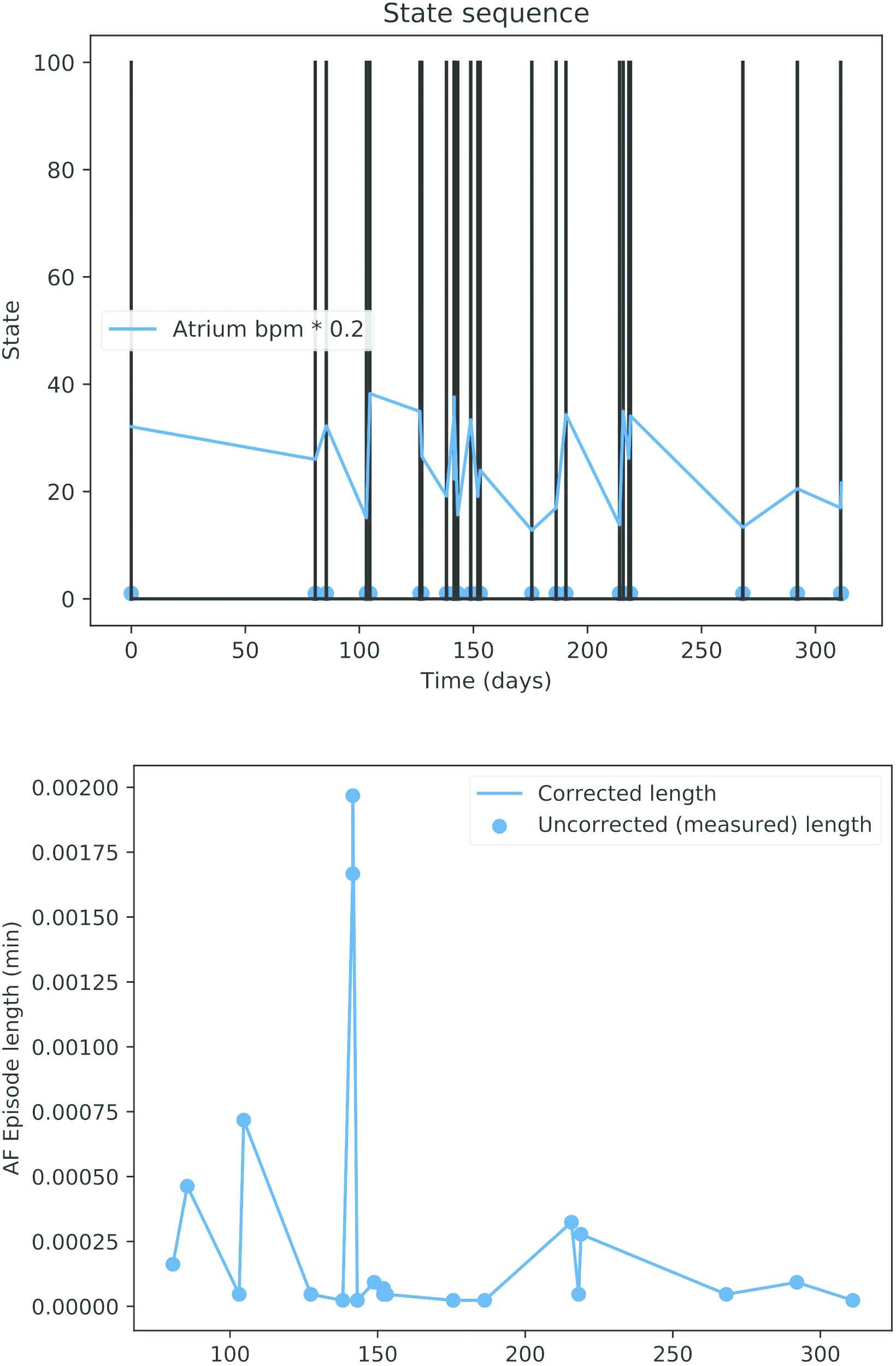
Top: Dates of pacemaker mode changes during a year. Bottom: Recorded length of the atrial fibrillation (AF) episodes.
There are also technical difficulties [10]. The algorithm that the ICD uses for detecting AF episodes depends on certain parameters that are adjusted by the technician on the basis of the iECGs mentioned before. Safety concerns prevail, thus the rate of false positives is high. As a consequence of this, long AF episodes are often reported as clusters of short episodes and a nontrivial preprocessing is needed to remove spurious events. This kind of preprocessing shortens the lists of episodes even more.
Because of the reasons mentioned before, the progression of AF is a complex process that depends on many different factors, but each patient will be associated to only a few tens of pacemaker records. There are not many different techniques for classifying short time series [11] and, according to our own experimentation, none of them is capable of finding a reliable break point between paroxistic and permanent AF.
The solution that is proposed in this paper consists in a generative map: a generative model produces data that is used to train a topology-preserving map, where the distances between the inputs are correlated with the distances between their projections in the map [12]. The topological map can be derived either from the activation of a single multi-class classifier or from an ensemble of binary classifiers. In the latter case, each of the binary classifiers is only exposed to arrhythmias of a certain type. When this array is fed with ICD records from a real patient, it is expected that only a few of these classifiers will react, meaning that the patient's arrhythmia is of the same type as the arrhythmia with which these classifiers were trained.
Most AI-based systems have a black-box nature that allows powerful predictions, but cannot be explained directly. For this reason explainable AI (XAI) has been gaining increasing attention recently. Layer-wise Relevance Propagation [13] is used as a proposal to understand classification decisions of nonlinear classifiers using heat maps that show the contribution of each pixel in computer vision applications. Class Activation Map (CAM) [14] has been also a popular method to generate saliency maps that highlight the most important regions in the data for making predictions, usually images. This concept has been applied in medical diagnosis [15]. Other methods rely on localization, gradients, and perturbations under the category of sensitivity [16,17]. Our method can be considered as a mixture of the latter and CAM. We project a visualization of the data using the activations of the neurons of the studied methods as a base to build these maps. The location of these activations will be arranged on the map to provide an intuitive visual diagnosis.
AF episodes are sequential data. Recurrent Neural Networks (RNNs) have been used in the literature in recent years for this type of problem and typically architectures such as Long Short-Term Memory (LSTM) [18] or Gated Recurrent Unit (GRU) [19] have proven to be good alternatives. On the other hand, a deep neural net architecture known as Generative Adversarial Network (GAN) [20] is currently breaking into Machine Learning in many fields [21–23]. Nonetheless, its research in the medical field is still limited [24,25], and their application for the diagnosis of cardiovascular diseases has not been explored yet.
Figure 3 presents a summary of the operation mode followed to give a better overall understanding:
A generative model(1) is used to simulate real clinical data(2).
The generated data is used for training different methods(3) to evaluate intracardiac records. Among these methods, further research is done to obtain a time series classifier based on adversarial training.
A self-explanatory graphic map(4) is obtained when the proposed methods are fed with data from real patients with AF.
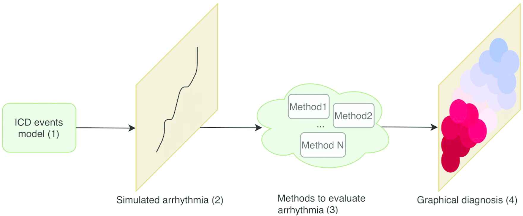
Pipeline of the presented work.
The structure of this paper is as follows: in Section 2, the generative model of the AF episodes are described. In Section 3, different approaches to solve the problem are presented. Performance of the different methods is discussed in Section 4. Visual representations and assessments are reported in Section 5 while conclusions are drawn in Section 6.
2. MODEL OF THE SEQUENCE OF ICD EVENTS
The purpose of this study is to predict the progression of paroxysmal cardiac arrhythmia to permanent AF on the basis of iECGs and other data collected by ICDs. AF episodes are easily detected in surface electrograms (ECGs) but iECGs are less informative. ECGs are representations of cardiac electrical activity from two electrodes placed on the surface of the body which are located apart from the heart (recall Figure 1, upper part). With this type of derivation, all kinds of electrical activity are recorded, including noncardiac electrical activity. On the contrary, iECGs (Figure 1, lower part) are representations of the potential difference between two points in contact with the myocardium in space over time.
2.1. AMS Events
ICDs do not store a continuous stream of data, but there are certain events that trigger that data is recorded. The primary purpose of an ICD is to release an electrical current between two points to activate the cardiac cells and therefore facilitate cardiac contraction. Depending on the electrical signal that is measured through the leads, the pacemaker will respond in order to stimulate, inhibit, or change its operation mode. In particular, in the presence of cardiac arrhythmia, if a patient experiences a high intrinsic atrial heart rate the pacemaker does not try to match the ventricle to the atrial rate. Instead, the pacemaker changes its operation mode and uses a different algorithm for generating the excitation of the ventricle. This process is called Automatic Mode Switching (AMS) [26]. AMS events are stored in the pacemaker memory and are used to mark the beginning of AF episodes (Figure 2, upper part). The lengths of the AF episodes are stored along with the AMS dates in the pacemaker memory.
Although AMS is a simple concept, the mode switching depends on a large number of variables that depend on the patient. It is possible that the pacemaker algorithm prematurely concludes that the AF event has ended, only to discover past a few seconds that an AF is still taking place. In this case, a second AMS event is generated and the pacemaker mode is restored. This has not relevant consequences for the efficiency of the device, but the stored information is inaccurate, as there may be cases where a cluster of short arrhythmias is reported instead of a long event.
2.2. Markov Model
The proposed dynamical model of the operation of an ICD is depicted in Figure 4. There are three states: “Normal,” “Arrhythmia,” and “False Normal.” A patient is in “Normal” state until an AMS event is issued by the ICD and the patient transitions to state “Arrhythmia.” There are two possible paths from this state: back to “Normal” when the episode ends or a transition to “False Normal” when a spurious end of episode is issued. In this second case, the patient remains in the state “False Normal” until a new AMS event is dispatched and then goes back to “Arrhythmia.” AMS events mark either the beginning of a true AF episode or the end of a “False Normal” state. This second class of AMS events are abnormal and should be purged, but there is not a simple procedure to remove them from ICD data [26]. Given that these events will be present in actual patients, the generative model must produce these spurious events as well.
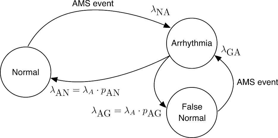
State diagram of the dynamical model of the beginning of atrial fibrillation (AF) episodes.
It will be assumed that the dates of the AF episodes conform an inhomogeneous Poisson process. The time between two episodes follows an exponential distribution with parameter
From a formal point of view, this model is a continuous-time Markov process that is characterized by a tuple of five parameters: (
3. GENERATIVE MAP
The diagnosis tool that is introduced in this study is a color-coded generative map that displays the actual state of the patient and the speed of change in his/her condition from paroxysmal to permanent AF. When the input is a Monte-Carlo simulation of AMS events, only a small area in the map should become active; ideally just one point. Otherwise, when actual AMS events are used, a potentially larger area could activate because ICD data will not match the output of any model in a perfect way. In other words, the activation area in the map is small when the diagnostic is clear and large when many different diagnostics are compatible with the available data. In this respect, the map can be regarded as a projection of the ICD data in an space whose coordinates are the values of
3.1. Uncertainty in the Data
Because of the behavior of the ICDs mentioned in the preceding section, spurious AMS events can be produced and it is possible that a long AF episode is perceived as a series of short events. There is not an easy procedure for knowing whether a non-simulated patient is in “Normal” or “False Normal” state.
In this study we will cope with this uncertainty by means of a fuzzy postprocessing that replaces the list of ICD logs by a continuous-time function that can be sampled at regular intervals. This transform consists in computing the degree of truth of the assert “the patient was undergoing an AF episode at time
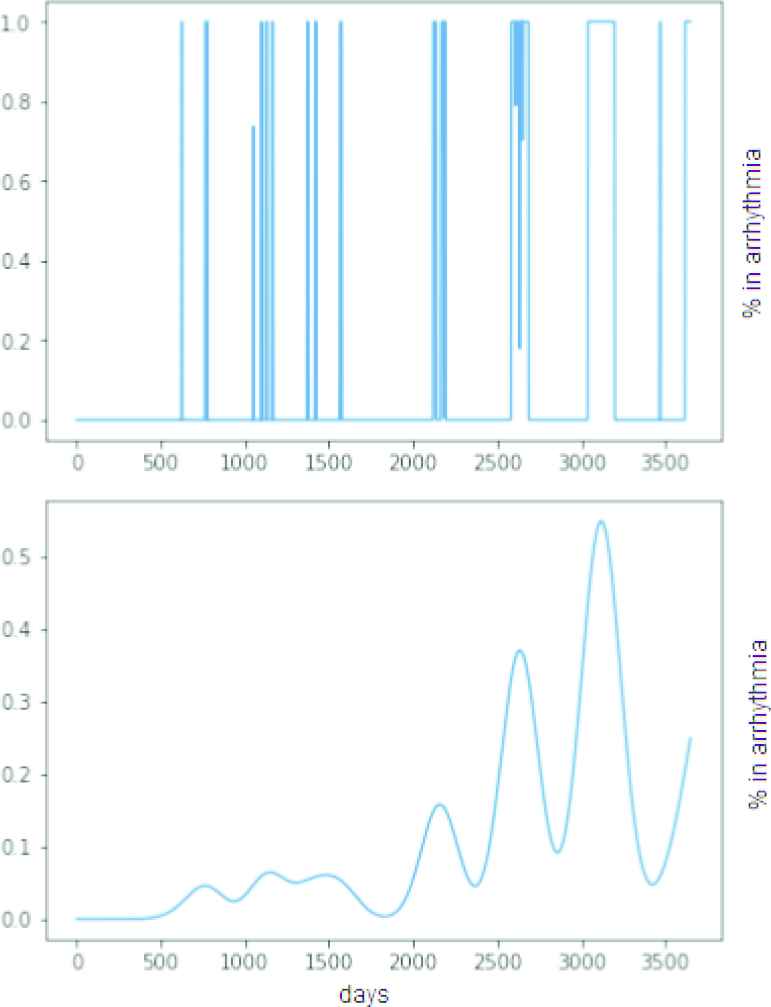
Top: Synthetic sequence of episodes (simulation time: 10 years). Bottom: Continuous-time function measuring the degree of truth that the patient is undergoing an arrhythmia episode at time.
3.2. LSTM and GRU Networks. Error Minimization and GAN Architecture
Networks are sought that are able to estimate the parameters of the Markov model given a truncated sample of postprocessed ICD events. RNNs are arguably the technique of choice for this application [28]. Let us remark that the difficulty of the problem at hand is learning from short time series, i.e., from incomplete information. The shorter the sample is, the more probable is that different models can produce the same sample.
Accurate and specific RNNs are sought. In our context, accuracy measures how often the net reacts to AF episodes similar to those in the training set. Specificity measures how different two models must be for the net being able to separate one from the other. The quality of the map depends on the RNN having the right amount of specificity: if the classifiers are too specific, there will be patients that are not visible in the map. If the specificity is too low, different parts of the map will be visible at the same time and the diagnosis will not be useful either.
LSTMs and GRUs are the most commonly used RNNs for classifying time series. In both cases, the input is distributed over a chain of cells and the main differences with previous RNNs are in the operations carried out within each cell, which will allow maintaining or forgetting information. LSTM cells consist of three gates: input, forget, and output gate. These multiplicative gates learn to manage the information passed so each memory cell decides what to store. GRU networks differ mainly in the number of gates: GRUs have two gates (input and forget gates are combined into a single gate) instead of three, which means lighter storage and faster training. Although LSTM has the ability to remember longer sequences, GRUs exhibit better performance on certain tasks [29,30], which makes us to consider them as an alternative for short-time series.
Training data is comprised by the postprocessed continuous-time functions defined in Section 3.1. In turn, two different methods were considered for training the RNNs:
Error minimization: the networks are trained for minimizing the squared error between the output of the net and the parameters of the Markov model. Alternatively, a set of clusters can be defined in the space of parameters of the model and the problem redefined as a multi-class classification task. The clusters in the space of parameters represent medical cases of interest, such as paroxysmal stable AF, paroxysmal AF with slow evolution to permanent AF, paroxysmal AF with quick evolution to permanent AF, permanent AF, and others. In this case, the concepts “accuracy” and “specificity” can be traced down to the confusion matrix of the classifier.
GANs: LSTMs or GRUs can be configured as GANs (see Figure 6.) GANs consist of 2 RNN: a generative net and a discriminative net. The generator net produces new data instances from noise, while the discriminator receives real data and the data from the generator and decides whether the generator's data belongs to the same distribution as the real data. From this verdict, the parameters of both networks are adjusted to improve in the next iteration until the generator is able to produce realistic data, that is to say, sequences of arrhythmia episodes. If a GAN is trained with arrhythmias with specific features a discriminator will be obtained that separates arrhythmias of that type from any other kind of arrhythmia. It is remarked that for this particular application we are not interested in the generative network, that is discarded after training (because the generative model introduced in Section 3.1 fulfills this function) but in the discriminative element. This process is repeated for each of the clusters in the space of parameters. A different GAN discriminator is learned for each class, and the generative map is the output of an ensemble that combines all the nets.
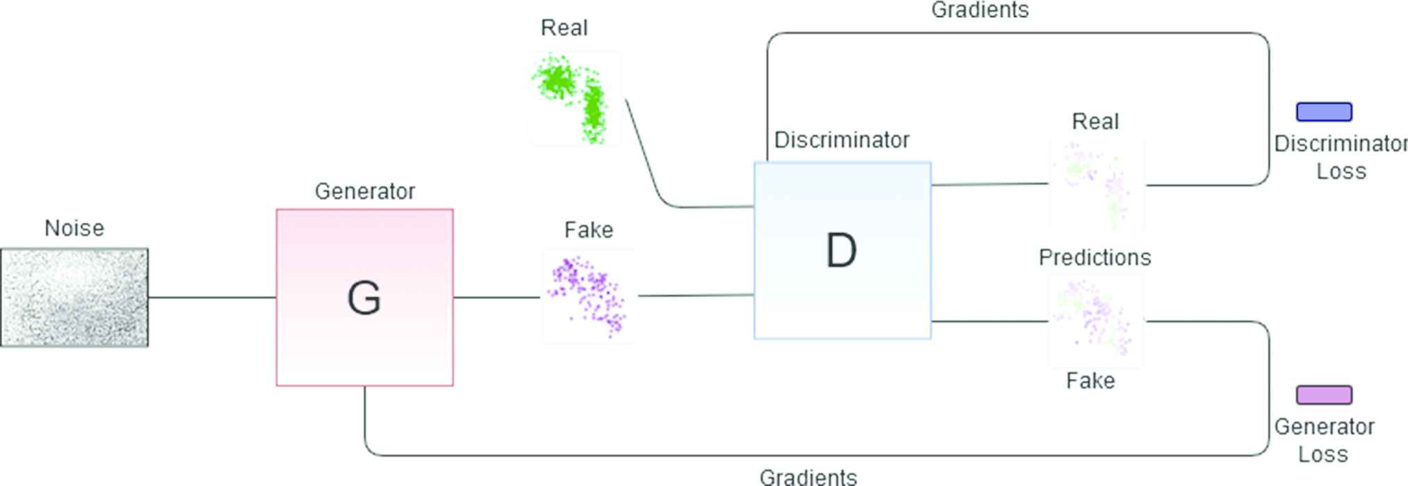
Generative adversarial network (GAN) architecture for obtaining one of the discriminant elements. The red block represents the generator net which generates fake data that is passed to the discriminator (blue block). The latter decides what is true and what is false from the input data and the gradients are adjusted according to the true labels until a discriminator that knows exactly what type of arrhythmia that is being trained with is obtained.
4. NUMERICAL RESULTS
The experimental validation of the proposed generative map has two parts. First, synthetic data with known properties is used to assess each of the presented alternatives. Second, actual patients are diagnosed, and their maps are validated by a human expert.
The experimental setup is described first. Second, the specificity of the GAN architecture is analyzed. In third place, the properties of LSTM and GRU networks are compared to that of GAN and also to non-neuronal classifiers. Fourth and last, some representative real-world cases are discussed.
4.1. Experimental Setup
The experimental setup is as follows: the code for training GAN recurrent networks for time series has been adapted from the publicly available code at https://github.com/ratschlab/RGAN [31].
A total of 14000 sequences have been generated for each combination of parameters chosen (60% was used for training, 20% for validation, and remaining 20% of data was used for testing). For multi-class problems, a softmax activation function is applied to the last layer of the LSTM- and GRU-based solutions in order to predict the class for the given pacemaker data. For GANs, each discriminator of the ensemble has its output passed through a sigmoid to determine whether the input belongs to the distribution data with which it was trained. Then all discriminator outputs are compared to determine which is the predicted class for the input.
4.2. Sensibility of the GAN-Based Approach
A brief study about the sensibility of the GAN-based maps has been included in Tables 1 and 2. The first table collects the results for
| Train | 0.9794 | 0.9804 | 0.9830 | 0.9868 | 0.9800 |
| Test | 0.9779 | 0.97978 | 0.9811 | 0.9847 | 0.9797 |
| 0.5299 | 0.2523 | 0.5373 | 0.4324 | 0.4878 | |
| 1.0000 | 1.0000 | 0.9979 | 0.3475 | 0.4424 | |
| 0.3333 | 1.0000 | 1.0000 | 1.0000 | 1.0000 | |
| - | 0.8162 | 1.0000 | 1.0000 | 1.0000 | |
| 0.9967 | - | 0.9505 | 0.9970 | 0.9983 | |
| 1.0000 | 0.9703 | - | 0.1369 | 0.1969 | |
| 1.0000 | 0.9994 | 0.0914 | - | 0.0312 | |
| 1.0000 | 1.0000 | 0.1494 | 0.0008 | - |
Sensitivity of the discriminator for
| Train | 0.9832 | 0.9823 | 0.9809 | 0.9825 | 0.9838 |
| Test | 0.9821 | 0.9818 | 0.9818 | 0.9853 | 0.9783 |
| 0.9986 | 0.9987 | 0.9986 | 0.9986 | 0.9997 | |
| 0.9998 | 0.9998 | 0.9956 | 0.9485 | 0.9809 | |
| 0.1543 | 1.0000 | 1.0000 | 1.0000 | 1.0000 | |
| - | 1.0000 | 1.0000 | 1.0000 | 1.0000 | |
| 1.0000 | - | 0.9988 | 0.9997 | 0.9996 | |
| 1.0000 | 0.9978 | - | 0.1703 | 0.2002 | |
| 0.9800 | 0.9800 | 0.0012 | 0.0516 | 0.0566 | |
| 1.0000 | 1.0000 | 0.0001 | - | 0.0357 | |
| 1.0000 | 1.0000 | 0.0000 | 0.0008 | 0.0089 |
Sensitivity of the discriminator for
The meaning of the rows and columns of these tables is as follows: each column contains the fraction of correct classifications of a discriminator that has been trained with sequences produced by the generative model. The values of
These results show that the nets are highly responsive when the arrhythmia is paroxysmal (low values of
4.3. Compared Results
In this section, 6 of the 10 AF categories used in the preceding subsection are used. These classes are labelled 998na10, 998na30, 998na180, 999na10, 999na30, and 999na180. The class labels begin with the first three decimals of
The different RNNs discussed in the preceding section are compared between them and also to two other standard nondeep learning classification methods, that have been included as a baseline: Multilayer Perceptron (MLP) and Random Forest. Table 3 collects the performance of the different models for each different class in terms of accuracy, i.e., each entry in Table 3 is the number of times that a series that was generated by the correct model was recognized as such. Also, to illustrate the performance of each method the ranking computed by Friedmans method for each dataset and the averaged resulting ranking is added.
| Accuracy |
|||||
|---|---|---|---|---|---|
| MLP | Random Forest | GRU | LSTM | GAN Ensemble | |
| 998na10 | 0.9921 (3) | 0.9918 (4) | 0.9964 (1) | 0.9943 (2) | 0.9782 (5) |
| 998na30 | 0.9654 (5) | 0.9857 (3) | 0.9911 (1) | 0.9875 (2) | 0.9686 (4) |
| 998na180 | 0.9371 (5) | 0.9800 (3) | 0.9879 (1) | 0.9946 (2) | 0.9596 (4) |
| 999na10 | 0.9739 (5) | 0.9943 (3) | 1.0000 (1.5) | 1.0000 (1.5) | 0.9803 (4) |
| 999na30 | 0.9368 (5) | 0.9979 (3) | 0.9996 (1.5) | 0.9996 (1.5) | 0.9911 (4) |
| 999na180 | 0.9911 (5) | 0.9946 (3) | 0.9982 (1) | 0.9957 (2) | 0.9796 (5) |
| Summary Results | |||||
| Accuracy | 0.9661 | 0.9907 | 0.9955 | 0.9953 | 0.9762 |
| Average rank | 4.6666 | 3.1666 | 1.1666 | 1.8333 | 4.3333 |
Note: AF, atrial fibrillation; MLP, multilayer perceptron; GRU, gated recurrent unit; LSTM, long short-term memory; GAN, generative adversarial network.
Accuracy of the different classifiers, six types of AF.
Observe that in all cases RNNs improve the results of MLP and Random Forest. In terms of accuracy, GRU is the RNN that better exploits the incomplete information in truncated ICD event series. It is better than MLP, Random Forest, and GAN with a p-value lower than 0.012 (according to Bonferroni correction [32]), followed by LSTM, although the difference is not statistically significant. LSTMs in GAN configuration apparently do not improve simpler classifiers such as Random Forest but their specificity is better and this metric has a higher impact in the visual coherence of the map. This point will be made clearer in Subsection 4.4. Observe also this metric is heavily dependent on the chosen division of the AF in clusters. To illustrate this fact, in Table 4 the same experiments carried out in Table 3 were repeated for a division in 8 classes (class labels 998na90 and 999na90 were added, with 90 days between AF episodes). The new classes are not easily separated from those with 180 days and the mean accuracy of the classifiers decreases.
| Accuracy |
||
|---|---|---|
| GRU | LSTM | |
| 998na10 | 0.9982 | 0.9968 |
| 998na30 | 0.9764 | 0.9796 |
| 998na90 | 0.8343 | 0.8529 |
| 998na180 | 0.8754 | 0.8464 |
| 999na10 | 1.0000 | 0.9982 |
| 999na30 | 0.9989 | 0.9975 |
| 999na90 | 0.8521 | 0.8904 |
| 999na180 | 0.9471 | 0.9286 |
| Summary Results | ||
| Accuracy | 0.9353 | 0.9363 |
Note: AF, atrial fibrillation; GRU, gated recurrent unit; LSTM, long short-term memory.
Accuracy of LSTM and GRU, eight types of AF.
Observe that the visual perception is much different if, e.g., a patient whose AF episodes occur every 180 days is assigned 90, 30, or 10 days. In order to keep the perceptual coherence the cost of misclassifying arritmias must not be uniform. This will be illustrated too in Section 4.4. In this respect, Figure 7 contains the confusion matrices of GAN (left) and Random Forest (right) for the initial division in six AF types. Observe that the number of correctly classified series is better for Random Forest, as expected, but there are two cells with errors that cannot be accepted from the medical diagnosis point of view: the cell 998na10- 999na10 (wrong rate of evolution for the same time between episodes) and, of secondary importance the cell 998na30- 999na180 (wrong rate of evolution and the initial time between episodes in the fast case is higher).
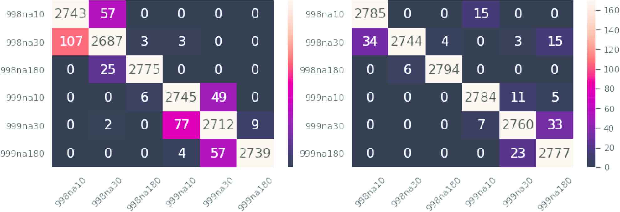
Left: Generative adversarial network (GAN) ensemble confusion matrix. Right: Random Forest confusion matrix. Similar classes are nearby on the map, thus errors in prediction should be close to the diagonal.
Observe that this behavior can be corrected if a cost matrix is introduced in the problem, although the problem of choosing the best cost matrix remains. For instance, if the cost matrix
4.4. Graphical Representation and Discussion
Three different experiments will be carried in this section. First, maps generated with different architectures (GAN and minimal error) are compared on data generated by the model. Second, two maps with minimal error and different clusterings of the generative model parameters are compared. Third, a true patient will be diagnosed by a human expert and by means of the proposed map.
4.4.1. Random forest versus LSTM-GAN
Two maps (see Figure 8) were selected for illustrating the differences between maps comprising RNNs and maps comprising other classifiers. The left map was obtained with an LSTM in a GAN configuration. The map in the right panel of the same figure was derived from a Random Forest. The horizontal axis is labelled
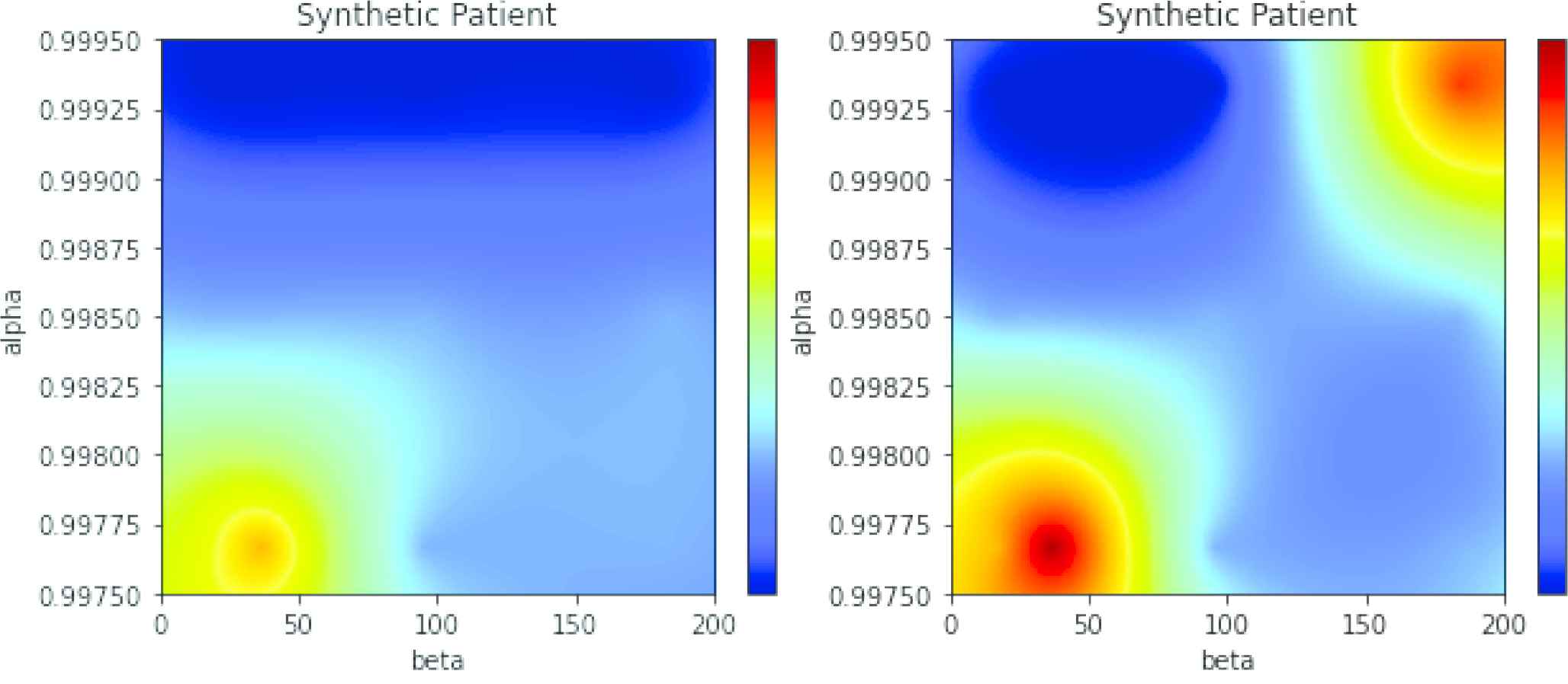
Left: Generative adversarial network (GAN) map for simulated atrial fibrillation (AF) alpha = 0.998, beta = 30. Right: Random Forest-based map for the same data.
Data is a random sample of the model with parameters
4.4.2. Effect of the different clustering in the generative model parameters
In Table 4 we shown that the division of the AF in categories influenced the accuracy of the RNNs. In Figure 9 two LSTM-based maps are compared. In the left panel, AF is divided into the six categories 998na10, 998na30, 998na180, 999na10, 999na30, and 999na180. In the right panel of the same figure the two additional categories were added, named 998na90 and 999na90. These two categories are harder to separate and the global accuracy decreases. The resulting maps are correct (both maps have maximum activations centered at
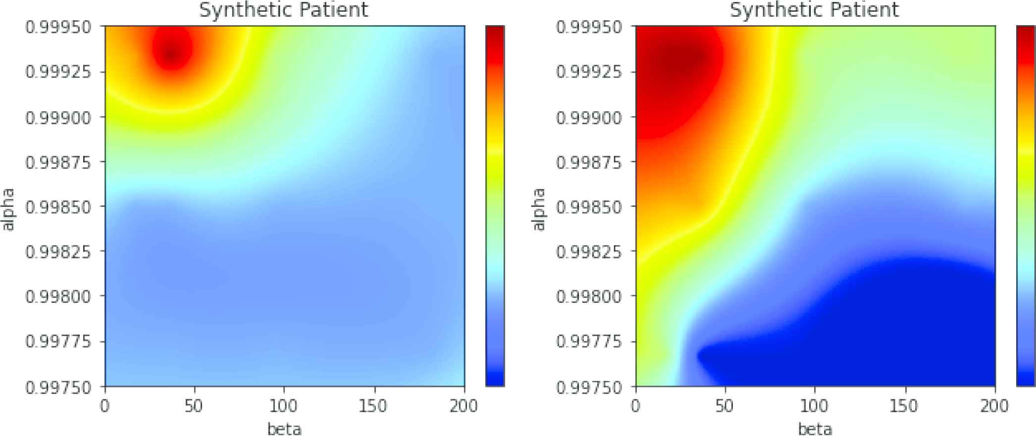
Left: Long short-term memory (LSTM)-based map, 6 clusters of atrial fibrillation (AF). Generative model with. Right: Same data, 8 clusters of AF.
4.4.3. Diagnosis of an actual patient
Actual data downloaded from the ICD of a patient with paroxystical arrhythmia is displayed in Figure 10. The black spikes are clusters of events (the isolated AMS events are not visible at this time scale). About three years of data are included in the figure. Observe that the time between events is higher in the first two years and the pace increases quickly in the last part (around the mark of the day 1000).

Dates of the automatic mode switching (AMS) events (black lines) and atrium beats per minute (bpm * 0.2) for an actual patient.
In Figure 11 three maps are displayed with the same conventions seen in the preceding subsection. The map in the left of the upper panel has been obtained with GRU, and map in the right in the same panel is produced by a LSTM network. The map in the bottom panel was obtained with another LSTM in GAN configuration. The three maps are similar and produce coherent results. The interpretation of these maps is as follows: the red region is centered in
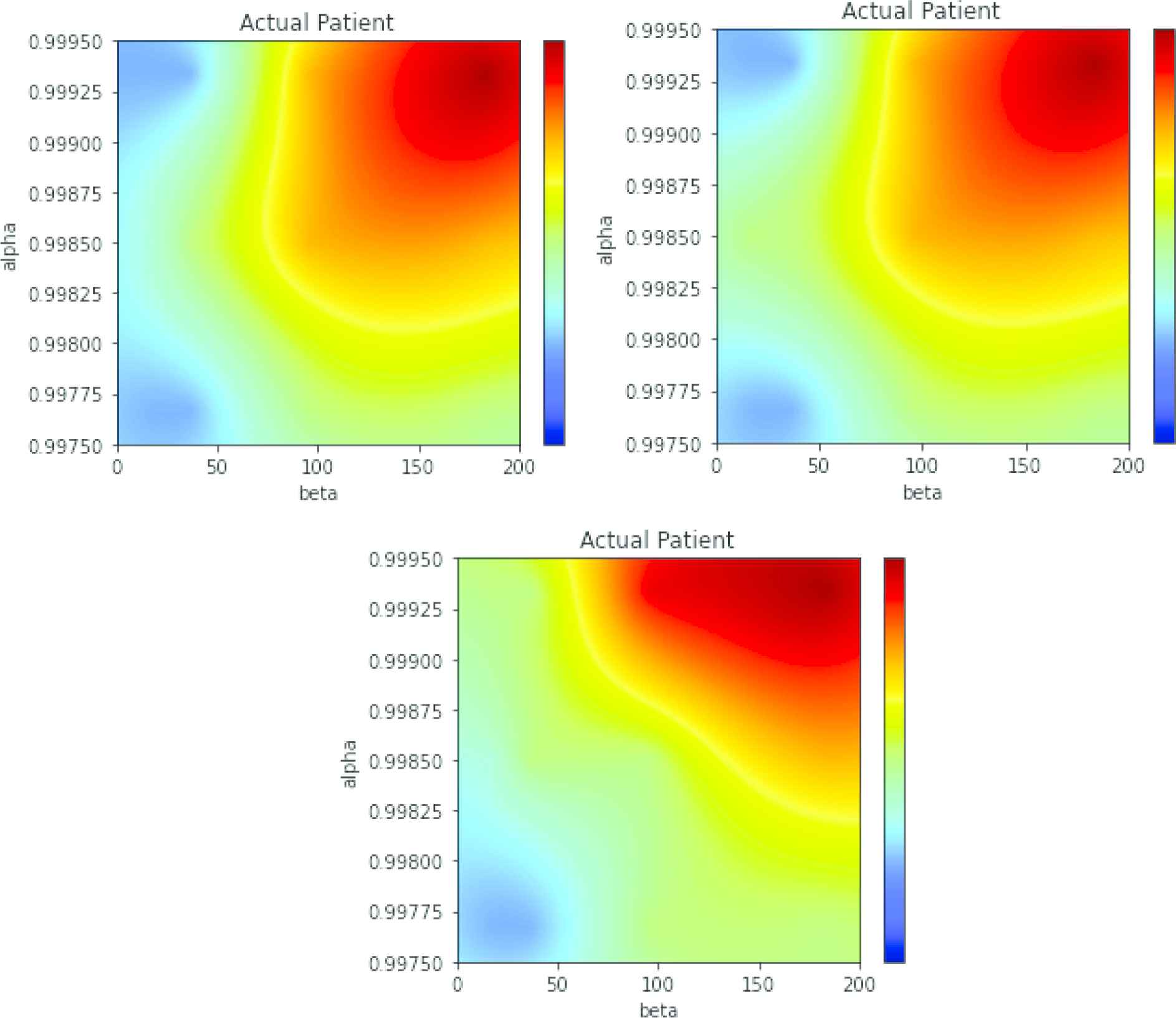
Maps of the patient in Figure 10. Top panel, left: multi-class gated recurrent unit (GRU). Top panel, right: multi-class long short-term memory (LSTM). Bottom panel: LSTM in generative adversarial network (GAN) configuration.
Observe that the map for an actual patient is not as specific as the maps obtained from data from the generative model. This means that it cannot be discarded that the patient has episodes every 3–4 months and his/her evolution is faster, up to a reduction factor of 0.58 per year. If Figure 10 is recalled, the number of episodes in the first 100 days was of three, but the following three episodes happened in more than one year, thus this kind of uncertainty in the diagnosis is correct, although the most probable diagnosis is that of a slow evolution.
5. CONCLUDING REMARKS AND FUTURE WORK
We have shown that iECGs from ICDs and pacemakers can be used to a certain extent for predicting the change from paroxysmal to permanent AF. The main difficulty is with the short length of the pacemaker records, that has been addressed here by means of a graphical projection of the sequence of AMS events in the parameter space of a generative model. If the data is enough for a clear diagnosis, the map produces an estimation of the patient condition and future evolution, and in those cases where the data is insufficient the map produces a set of estimations that can be subjectively assessed in order to determine whether the evolution is positive or not. Such a diagnosis can help specialists reduce the time spent analyzing intracardiac data.
LSTM and GRU have shown remarkable results as a standalone multi-class classifier, and LSTM was adequate as a part an ensemble of GAN detectors as well. GANs have an intrinsic advantage, that is the obtention of the generator network, that may be a better generative model than the continuous Markov model used in this study. If a number of ICD records of actual patients was high enough, it would make sense to bootstrap the model with the generative model described in this paper and fine-tune the GANs with real-world data, for obtaining an improved generative model. Such a GAN-based generative model could have an application on its own, as a predictor of future AF episodes. Lastly, we are currently working in other alternatives than GANs for obtaining the diagnostic map, such as the use of Variational Autoencoders, than can also be trained on model-generated data and be applied to ICD logs to get a compact representation of the evolution of AF.
CONFLICTS OF INTEREST
The authors declare no conflict of interest.
AUTHORS' CONTRIBUTIONS
Conceptualization: Nahuel Costa, Jesús Fernández, Luciano Sánchez; Methodology: Nahuel Costa, Luciano Sánchez; Software: Nahuel Costa; Validation: Nahuel Costa, Inés Couso.
ACKNOWLEDGMENTS
This work has been partially supported by the Ministry of Economy, Industry and Competitiveness (“Ministerio de Economía, Industria y Competitividad”) from Spain/FEDER under grant TIN2017-84804-R and by the Regional Ministry of the Principality of Asturias (“Consejería de Empleo, Industria y Turismo del Principado de Asturias”) under grant GRUPIN18-226.
REFERENCES
Cite this article
TY  - JOUR
AU  - Nahuel Costa
AU  - Jesús Fernández
AU  - Inés Couso
AU  - Luciano Sánchez
PY  - 2020
DA  - 2020/10/06
TI  - Graphical Analysis of the Progression of Atrial Arrhythmia Using Recurrent Neural Networks
JO  - International Journal of Computational Intelligence Systems
SP  - 1567
EP  - 1577
VL  - 13
IS  - 1
SN  - 1875-6883
UR  - https://doi.org/10.2991/ijcis.d.200926.001
DO  - 10.2991/ijcis.d.200926.001
ID  - Costa2020
ER  -