Fuzzy initial value problem; Sup-J extension principle; Interactive fuzzy numbers; Chemical reactions
Abstract
This paper studies numerical solutions for fuzzy initial value problems, where the initial conditions are given by interactive fuzzy numbers. The fuzzy solution is given by a numerical method that employs the arithmetic of interactive fuzzy numbers and yields a fuzzy number at each instant of time. The computational cost of the numerical method is also provided. The chemical decay reaction model is considered in order to illustrate that different types of interactivity produce different solutions for initial value problems. In addition, we present an application to the Lotka–Volterra model of oscillating chemical reactions.
Chemical kinetics deals with experiments in chemistry and interprets them in terms of mathematical models. In particular, chemical kinetics studies chemical reactions, as well as the factors that influence the final result [1]. Chemical reactions are transformations that involve changes in the bonds of the particles of matter, resulting in the formation of a new substance with different properties than the previous one [2]. A chemical decay of a reagent is an example of a chemical reaction:
A→kB,with reaction rate k.(1)
Here A is the initial reagent and B is the final product.
A reaction is said to be reversible if reagents transform into a product and the product transforms into a reagent, simultaneously reaching an equilibrium [1]. Otherwise, the reaction is said to be irreversible. The chemical decay given by (1) is an example of irreversible reaction.
This paper focuses on chemical reactions of the type U+V→cW, where U and V are the consumed reagents and W is the final product of this reaction, with proportion c.
Some factors may influence the velocity of these reactions, for instance, concentration, activation energy, temperature, pressure, and so on. The velocity (v) of a reaction can be determined from v=k[U]m[V]n, where k is the reaction rate, [U] and [V] are concentrations of the reagents and m and n are the orders of the reactions, which are determined experimentally. Although there may be imprecision (or uncertainty) in the process of obtaining these parameters, classical models do not consider this fact [3]. Note that fuzzy set theory can be used to describe this imprecision or uncertainty.
This paper focuses on the Lotka–Volterra model of oscillating chemical reactions which is based on a molecular mechanism where at each step the reagent molecules combine to produce intermediate reagents or final products. In 1920, Lotka [4] proposed the following reaction mechanism [5]:
Each step of (2) refers to the molecular mechanism, where the reagents combine to produce intermediate reagents or products. For instance, the first step describes the molecules of A combining with the ones of X to produce two molecules of X. This step depletes the molecules of A, and adds molecules of X, at a rate proportional to the product of the concentrations of A and X, given by k1 [4].
The effective rate laws for the reagent A, the product B, and the intermediate reagents X and Y are described by the initial value problem (IVP) [6]
It is worth noting that the sum of concentrations [A(t)],[X(t)],[Y(t)], and [B(t)] remains constant at every instant of time, that is,
[A(t)]+[X(t)]+[Y(t)]+[B(t)]=k,∀t∈ℝ(4)
for some k∈ℝ, since
d[A]dt+d[X]dt+d[Y]dt+d[B]dt=0.
In particular, this observation holds for the initial concentrations
[A0]+[X0]+[Y0]+[B0]=k.(5)
The initial conditions and/or parameters of the system (3) may be uncertain [3]. This paper focuses on the case where the initial concentrations are uncertain and modeled by fuzzy numbers. Hence, Equation (5) implies that the addition of some fuzzy numbers results in a real number.
It is well known in the literature that the standard sum of fuzzy numbers never yields a real number. Thus a special arithmetic of fuzzy numbers must be considered in order to guarantee that the total quantity (k), given in (4), is a real number. Barros and Santo Pedro [7] argued that only special cases of interactive arithmetic can have this property.
Interactivity is a relationship between fuzzy numbers that resembles the concept of dependence of random variables. In probability theory, the dependence (or independence) of random variables is defined in terms of a probability distribution. Similarly, in fuzzy set theory, the relation of interactivity arises from the concept of joint possibility distribution.
The motivation to use the concept of interactivity is twofold: the first one is to ensure that Equation (4) holds. The second one is to intrinsically model the dependence between the reagents/products and their concentrations [2].
An IVP whose initial conditions are given by fuzzy numbers is called fuzzy initial value problem (FIVP). Let us use the method proposed by Wasques et al. [8] in order to provide a numerical solution for the FIVP given by (3). This method which can be used for any n-dimensional system of differential equations consists in replacing the arithmetic operations of the classical Runge–Kutta method of order 1 (Euler) by arithmetic operations derived from the sup-J extension principle for interactive fuzzy numbers.
There are several numerical methods proposed in the literature. Ahmed et al. [9] proposed a new fuzzification of the classical Euler method and an optimization technique to provide this solution. Other approaches are based on the concept of fuzzy derivatives [10–13]. For example, Ahmadian et al. [10] proposed a numerical solution to FIVPs, based on the generalized Hukuhara differentiability and the Runge–Kutta method. All these methods and many others [14,15] are given in terms of α-cuts, using interval arithmetic. This procedure does not guarantee that the numerical solution produces a fuzzy number at each instant of time. In contrast, this paper shows that the numerical method of Wasques et al. [8] yields a fuzzy number at each instant of time, which is consistent with the fact that the analytical solution must be a fuzzy function.
Using an application to the chemical decay reaction, this paper illustrates that different types of interactivity result in different solutions for FVIPs. Finally, an application to the Lotka–Volterra model of oscillating chemical reactions clearly exhibits the dependence of the final result and the concentration factors.
The contributions of the present article, which represents an extended version of a recent conference paper [16], include the following:
We show that the proposed numerical method yields a fuzzy number at each iteration.
We analyze the computational complexity of the method.
We use several FIVPs, one of which cannot be found in [16], in order to illustrate how our method works.
2. MATHEMATICAL BACKGROUND
This section reviews Euler's method and some basic concepts of fuzzy set theory.
2.1. Euler's Method
Let yi:ℝ→ℝn, with i=1,…,n, be functions that depend on time t. Consider the ordinary differential equation (ODE) with initial value given by (6)
dyidt=fi(t,y1,y2,…,yn)y(t0)=y0∈ℝn,i=1,…,n,(6)
where fi:ℝn+1→ℝ depends on y1,y2,…,yn and t.
Euler's method consists in determining numerical solutions, that is, approximate values yik of yi at times t0,t1,…,tN, for ODEs described by (6), as follows:
yik+1=yik+hfi(tk,y1k,…,ynk).(7)
Here, tk+1−tk=h>0 for k=0,1,…,N−1 for some N∈ℕ and (t0,yi0) is the initial condition.
2.2. Fuzzy Set Theory
A fuzzy subsetA of a universe X is associated with a function A:X→[0,1] called membership function, where A(x) represents the membership degree of x in A for all x∈X. The symbol ℱ(X) denotes the class of fuzzy subsets of X. From now on, the set X is assumed to be a topological space.
The α–cut of a fuzzy set A⊆X, denoted by [A]α, is defined by
[A]α={x∈X:A(x)⩾α},0<α⩽1cl{x∈X:A(x)>0},α=0,
where clY denotes the topological closure of Y⊆X [17].
A fuzzy subset A of ℝ is called a fuzzy number if all α–cuts are bounded, closed and nonempty intervals for all α∈[0,1]. The α–cuts of the fuzzy number A are denoted using [A]α=[aα−,aα+]. The class of fuzzy numbers, denoted ℝℱ, represents a special class of fuzzy subsets of ℝ that includes the sets of the real numbers as well as the set of the bounded closed intervals of ℝ. In addition, the subclass ℝℱC is defined as the set of all fuzzy numbers such that the endpoints of its α-cuts are continuous as functions of α. For example, any interval [a,b] is an element of ℝℱC. Another example is a triangular fuzzy number. Recall that a triangular fuzzy numberA, denoted by the triple (a;b;c) for some a⩽b⩽c, has the following membership function:
A(x)=x−ab−a,a⩽x<bc−xc−b,b⩽x<c0,otherwise.
The α–cuts of triangular fuzzy numbers are given by [A]α=[a+α(b−a),c−α(c−b)],∀α∈[0,1].
The Hausdorff norm of fuzzy numbers is defined in terms of the levelwise metricd∞ [18]. This definition is given as follows:
Definition 1.
Let A and B be fuzzy numbers. The levelwise metricd∞:ℝℱ×ℝℱ→[0,+∞) is given by
d∞(A,B)=⋁α∈[0,1]max{|aα−−bα−|,|aα+−bα+|},
where ∨ stands for the supremum operator.
Moreover, the Hausdorff norm of a fuzzy number A∈ℝℱ is defined by
||A||ℱ=d∞(A,0),(8)
where the symbol 0 stands for the characteristic function χ{0} of the real number 0.
The definition of the width of a fuzzy number is provided as follows:
Definition 2.
The width (or diameter) of a fuzzy number A∈ℝℱ is defined by
width(A)=a0+−a0−.(9)
The width of a fuzzy number A is associated with the uncertainty that it models.
A fuzzy relation J∈ℱ(ℝn) is said to be a joint possibility distribution of fuzzy numbersA1,…,An∈ℝℱ if
Ai(y)=⋁(x1,…,xn):xi=yJ(x1,…,xn),∀y∈ℝ,(10)
for all i=1,…,n.
The t-norm-based joint possibility distribution is defined as follows. Let △ be a t-norm, that is, an associative, commutative and increasing operator △:[0,1]2→[0,1] that satisfies △(x,1)=x for all x∈[0,1]. The fuzzy relation J△ given by
J△(x1,…,xn)=A1(x1)△…△An(xn)(11)
is called the t-norm-based joint possibility distribution of A1,…,An∈ℝℱ.
If the t-norm is given by the minimum operator (△=∧), that is,
J∧(x1,…,xn)=A1(x1)∧…∧An(xn),(12)
then the fuzzy numbers A1,…,An are said to be noninteractive.
Definition 3.
The fuzzy numbers A1,…,An are said to be interactive, if their joint possibility distribution J satisfies (10) and J≠J∧.
Definition 3 reveals that the interactivity of the fuzzy numbers A1,…,An arises from a given joint possibility distribution.
There are some types of interactivity, such as complete correlation and linear interactivity, that are not based on t-norm-based joint possibility distributions. Complete correlation is one type of interactivity that was introduced by Fullér et al. [19,20], for two fuzzy numbers. Subsequently, the authors of [21,22] proposed an extension of this notion for n fuzzy numbers, where n>2, and they called this relation linear interactivity.
The fuzzy numbers A1,…,An are said to be linearly interactive, if there exists a joint possibility distribution J=JL and q2,r2,…,qn,rn∈ℝ that satisfy
for all (x1,…,xn)∈ℝn, where χL stands for the characteristic function of the set
L={(u,q2u+r2,…,qnu+rn):∀u∈ℝ}
for some qi,ri, where i=2,…,n.
The joint possibility distribution JL was used in several problems such as fuzzy differential equations [7,21,22] and least square problems [23,24]. However this joint possibility distribution can only be applied to fuzzy numbers that have a colinear relationship between their membership functions. This means that it cannot be used for fuzzy numbers that do not have the same shape. For example, the fuzzy numbers (0;1;2) and (1;2;3) are linearly interactive, in contrast to (0;1;2) and (1;2;5) which are not.
Let us present a more general joint possibility distribution that can be applied to every pair of fuzzy numbers.
Given A1,A2∈ℝℱC, for each z∈ℝ and α∈[0,1] consider the auxiliary functions g∧i, g∨i and vi defined by [25]
The set P(γ) defines the elements (x1,x2) such that Jγ(x1,x2)>0. Since P(γ)≠[A1]α×[A2]α=[J∧]α for all γ∈[0,1) and the α-cuts of Jγ are contained in the set P(γ), it follows that Jγ≠J∧, for all γ∈[0,1).
Esmi et al. [25] proved that Jγ, given by (14), is a joint possibility distribution of A1 and A2 for all γ∈[0,1]. The parameter γ implicitly models the “level” of interactivity between the fuzzy numbers A1 and A2, in the following sense: The lower the value of γ, the higher the interactivity.
Recall that for γ=1, it follows that J1=J∧ (see (12)) [25]. This means that if the chosen joint possibility distribution is J1, then one is dealing with noninteractive fuzzy numbers [25].
The following definition is a generalization of Zadeh's extension principle [26], which is used to extend classical functions to functions with fuzzy numbers as arguments.
Definition 4.
[19] Let J∈ℱ(ℝn) be a joint possibility distribution of (A1,…,An)∈ℝℱn and f:ℝn→ℝ. The sup-J extension of f at(A1,…,An)∈ℝℱn, denoted fJ(A1,…,An), is the fuzzy set given by
fJ(A1,…,An)(y)=⋁(x1,…,xn)∈f−1(y)J(x1,…,xn),(15)
where f−1(y)={(x1,…,xn)∈ℝn:f(x1,…,xn)=y} is the inverse image of the function f at y.
From Definition 4, it is possible to establish an arithmetic for interactive fuzzy numbers. This arithmetic is provided in Section 3.
3. INTERACTIVE ARITHMETIC FOR FUZZY NUMBERS
An interactive arithmetic arises from the sup-J extension principle, where the function f, given as in (15), is an arithmetic operator (+,−,∗,÷) and J is some joint possibility distribution such that J≠J∧. Interactive arithmetic operations are defined as follows:
Definition 5.
Let be A1,A2∈ℝℱ and J be their joint possibility distribution. Interactive arithmetic operations are defined by
(Sum)
(A1+JA2)(y)=⋁x1,x2:x1+x2=yJ(x1,x2).
(Difference)
(A1−JA2)(y)=⋁x1,x2:x1−x2=yJ(x1,x2).
(Product)
(A1∗JA2)(y)=⋁x1,x2:x1∗x2=yJ(x1,x2),
(Quotient)
(A1÷JA2)(y)=⋁x1,x2:x1÷x2=yJ(x1,x2).
(Multiplication by a scalar) Let be λ∈ℝ. Thus
λA1(y)=⋁x1:λx1=yA(x1).
Definition 5 implies that an interactive arithmetic depends on the joint possibility distribution J. Moreover, if J is given by J∧, that is, A1 and A2 are noninteractive, then the arithmetic provided by the sup-J extension principle boils down to the standard fuzzy arithmetic, that is, the arithmetic for fuzzy numbers that is obtained from the Zadeh extension principle. Note that the multiplication by a scalar, given by item (v), is the same scalar product as the one given by standard fuzzy arithmetic.
The following properties hold true for interactive arithmetic operations.
Theorem 1.
[27] LetA,B,C,D∈ℝℱandJ∧be the joint possibility distribution given by (12). For all joint possibility distributionsJand⊗∈{+,−,∗,÷}we have that
A⊗JB⊆A⊗∧B;
λ(A⊗JB)⊆λ(A⊗∧B), for allλ∈ℝ;
IfA⊆BthenA⊗JC⊆B⊗∧C;
IfA⊆BandC⊆DthenA⊗JC⊆B⊗∧D;
(A⊗J(B⊗JC))⊆(A⊗∧(B⊗∧C)).
This paper focuses on the interactive arithmetic that is obtained from the family of joint possibility distributions Jγ, since it generalizes JL [8]. Moreover, taking advantage of the fact that width(A)⩽2||A||ℱ for every A∈ℝℱ, Sussner et al. [28] employed shifts in order to define a new family of parametrized joint possibility distributions Jγc. These shifts can be obtained as follows.
Theorem 2.
GivenA1,A2∈ℝℱCandc=(c1,c2)∈ℝ2. LetÃi∈ℝℱCbe such thatÃi(x)=Ai(x+ci), ∀x∈ℝandi=1,2. LetJ̃γbe the joint possibility distribution of fuzzy numbersÃ1,Ã2∈ℝℱCdefined as in Equation (14). The fuzzy relationJγcgiven by
Jγc(x1,x2)=J̃γ(x1−c1,x2−c2),∀(x1,x2)∈ℝ2,(16)
is a joint possibility distribution ofA1andA2.
Proposition 3.
[28,29] LetJγcbe the joint possibility distribution of the fuzzy numbersA1andA2that is given by (16). The following statements are equivalent:
γ⩽β;
Jγc⊆Jβc;
A1⊗γcA2⊆A1⊗βcA2; and
width(A1⊗γcA2)⩽width(A1⊗βcA2).
This paper focuses on a particular choice of c=(c1,c2). From now on, the values ci are given by the midpoint of [Ai]1, for i=1,2. These particular choices of c1 and c2 allow to reach results with smaller widths than the ones obtained using Jγ. For example, we have that width((1;2;3)⊗J0c(1;2;3))=0<width((1;2;3)⊗J0(1;2;3))=2. To simplify, let us use the symbol ⊗γ to denote ⊗Jγc.
Proposition 3 ensures that the arithmetic operations have the minimum and maximum width at γ=0 and γ=1, respectively. The next example illustrates this result.
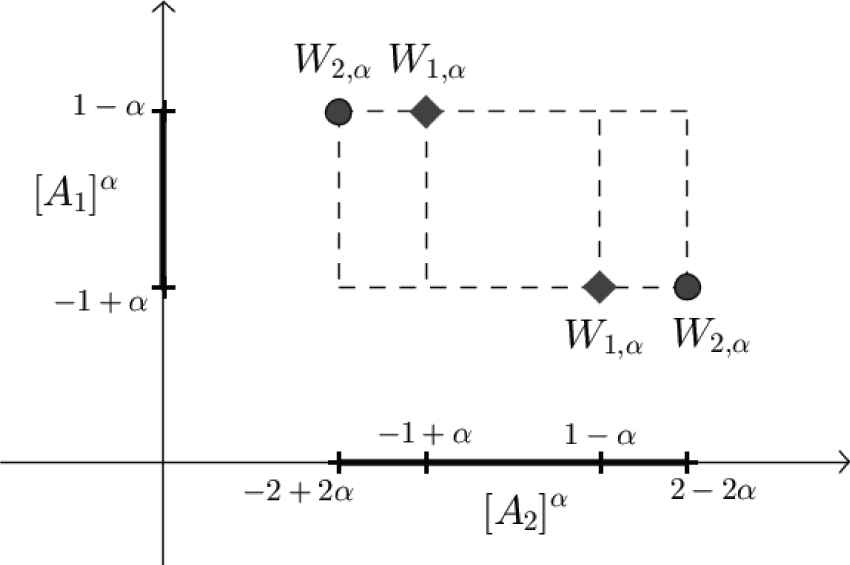
Example 1.
Consider A1=(−1;0;1) and A2=(−2;0;2). The interactive sum for γ=0 is given by
The sets W1,α and W2,α are depicted in Figure 1. The elements that are associated according to W1,α are visualized using lozenges. The elements that are associated according to W2,α are visualized using circles.
Figure 1
The domain P(0) of J0, for each α-cut, where [A1]α=[−1+α,1−α] and [A2]α=[−2+2α,2−2α]. The circles and lozenges represent the elements of the sets W1,α and W2,α, respectively.
Now, if (x1,x2)∈W1,α, then z=x1+x2=0. If (x1,x2)∈W2,α, then
Moreover, for γ=1 one obtains A1+1A2=(−3;0;3)=A1+A2, where the symbol “+” represents the standard sum on fuzzy numbers, corroborating the previous observation.
Example 2.
[30] If A1 and A2 are respectively the triangular fuzzy numbers (1;2;3) and (2;3;4), then
A1+0A2=5,
where 5 stands for the fuzzy number 5, whose membership function is given by the characteristic function χ{5}.
Example 2 reveals that the interactive sum of two fuzzy numbers in terms of Jγc may yield a real number. This implies that the interactive sum based on this family of joint possibility distributions can be used in order to satisfy Equations (4) and (5).
The interactive arithmetic via Jγc has another interesting property. The interactive difference, for γ=0, is equal to the generalized difference [31]. This means that the Hukuhara difference and its generalizations [32] are particular types of interactive arithmetic operations, and all these differences can be obtained from the interactive difference −0.
Section 4 provides the numerical solutions for FVIPs and a discussion about the advantages of this method in comparison to others given in the literature.
Since the initial condition Y0 is given by a fuzzy number, the arithmetic operations presented in (7) must be adapted for fuzzy numbers as suggested by Wasques et al. [8]. This paper considers the interactive arithmetic obtained from the family Jγc. An algorithm that produces a numerical solution to the FIVP (17) is given by
Yik+1=Yik+γhfi(tk,Y1k,…,Ynk).(18)
Note that in order to compute the right side of Equation (18) it is necessary that fi(tk,Y1k,…,Ynk)∈ℝℱC. For the case where fi is given in terms of interactive arithmetic operations ⊗γ, γ∈[0,1], such as the oscillating chemical reaction problem addressed in Section 6, we have that fi(tk,Y1k,…,Ynk)∈ℝℱC if Yi1∈ℝℱC for all i=1,…,n. From Theorem 2 of [25], we have that every iteration of the method produces a fuzzy number in ℝℱC. This fact is established in Proposition 4.
Proposition 4.
The fuzzy set given by Equation (18) is a fuzzy number inℝℱCfor alli=1,…,nand for all iterationk.
Theorem 1 implies that the numerical solution given by (18) is always contained in the solution given by the standard fuzzy arithmetic. In fact, this result holds true for all interactive arithmetics [27].
It is important to observe that for γ=1 the method produces a numerical solution with increasing width since width(Yik+1)⩾width(Yik) for all i=1,…,n. This implies that the method (18) propagates uncertainty if one uses standard fuzzy arithmetic.
Let us illustrate the above observations by considering the chemical decay reaction, which can be described by the following differential equation
d[A]dt=−d[A],[A(0)]=[A0],(19)
where d>0.
Suppose that the initial concentration [A0] is uncertain and described by a fuzzy number, that is, [A0]∈ℝℱ. Thus, the numerical solution for (19) is determined as follows:
[Ak+1]=[Ak]+γh(−d[Ak]).(20)
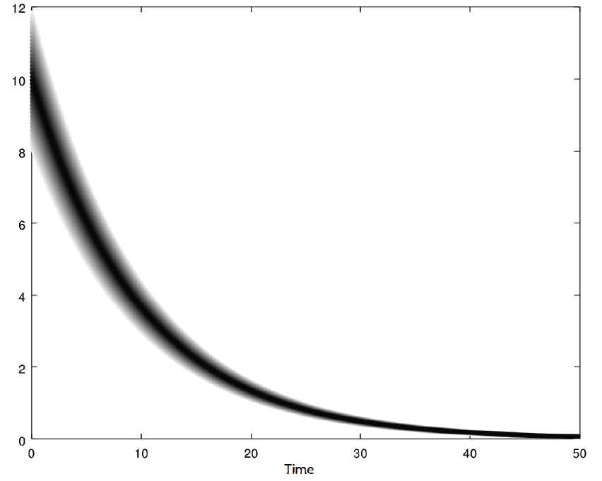
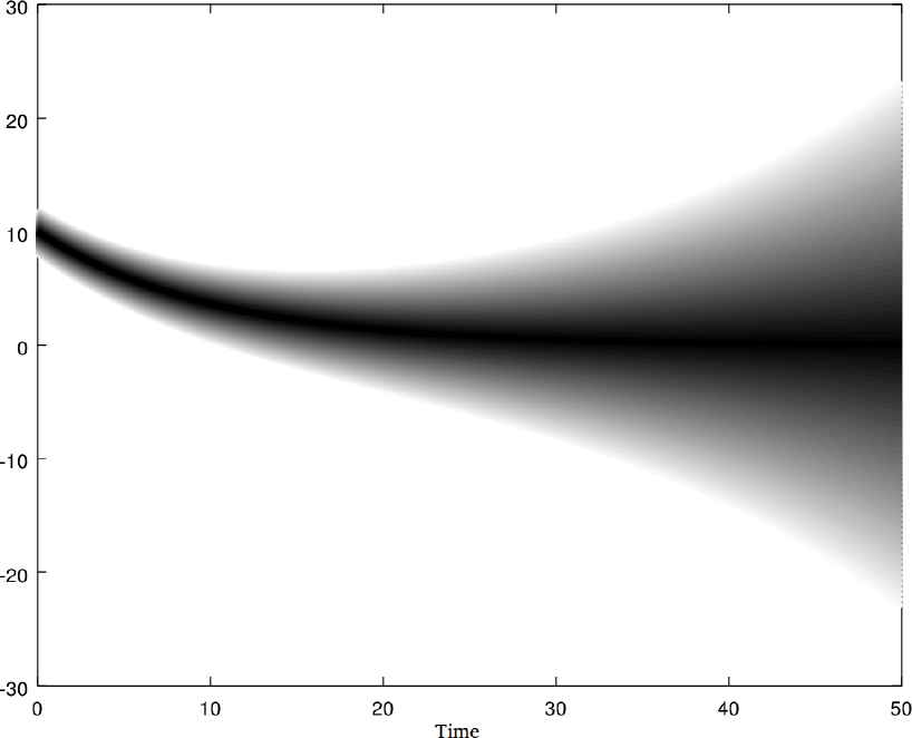
The numerical solutions given by (20) are depicted in Figures 2, 3 and 5, for some values of γ. Figure 6 illustrates the numerical solution based on the standard fuzzy arithmetic. The parameters are given by [A]0=(8;10;12), d=0.1 and h=0.125. In these figures, the α-cuts of the fuzzy solutions for α varying from 0 to 1 are represented using shades of gray with increasing darkness.
Figure 2
Numerical solution to the chemical decay reaction given by Equation (19) for γ=0. Here, we used [A]0=(8;10;12), d=0.1 and h=0.125.
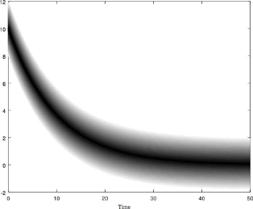
Figure 3
Numerical solution to the chemical decay reaction given by Equation (19) for γ=0.5.
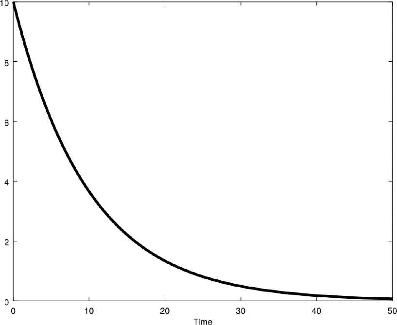
Figure 4
Classical numerical solution to the chemical decay reaction given by Equation (19). The initial condition is given by [A]0=10.
Figure 5
Numerical solution to the chemical decay reaction given by Equation (19) for γ=0.75.
Figure 6
Numerical solution to the chemical decay reaction given by Equation (19) for the standard fuzzy arithmetic, which coincides with the numerical solution for γ=1.
Note that the numerical solutions given by γ=0 and γ=0.5 present a similar qualitative behavior as the deterministic solution, depicted in Figure 4. In other words, both deterministic and fuzzy solutions decrease over time.
Also, observe that the numerical solution for γ=0.75 is very similar to the solution given by the standard fuzzy arithmetic. Both solutions have increasing width over time. This fact is due to the value of γ, which is close to γ=1.
Thus, for the chemical decay reaction, given by (19), the numerical solutions depicted in Figures 2 and 3 may be more appropriate in order to describe the evolution of the decay, in the case the initial concentration is uncertain. From the modeling point of view, the numerical solution, for γ=0.75, is not appropriate to describe the evolution of the decay, since it propagates uncertainty as well as the numerical solution obtained from the standard fuzzy arithmetic.
It is interesting to observe that the numerical solution for γ=0.75 contains the numerical solution for γ=0.5, which contains the numerical solution for γ=0, as illustrated in Figure 7. This fact corroborates the result given by Item (iii) of Proposition 3.
Figure 7
Comparison of the numerical solutions to the chemical decay reaction given in Equation (19). The blue, red, green and black lines represent the 0-cut of the numerical solutions for γ=0, γ=0.5, γ=0.75, and γ=1, respectively.
Note that the width of the numerical solution given by γ=0 is less or equal than the width of the other numerical solutions, for all instants of time. This fact corroborates the result given by Item (iv) of Proposition 3.
Next, we present some important remarks regarding the proposed numerical solution.
Remark 1.
The method (18) produces a fuzzy number, for each iteration k;
The method (18) requires that Yik and hfi(tk,Y1k,…,Ynk) are interactive with respect to some joint possibility distribution J, for each iteration k;
All the arithmetic operations in the method (18) must be interactive.
In general, the methods proposed in the literature are determined in terms of α-cuts, boiling down to a study of classical theory. Thus the Negoita–Ralescu representation theorem must be satisfied in order to guarantee that the solution is a fuzzy number at every instant of time. However, this condition is not verified in the most of these methods.
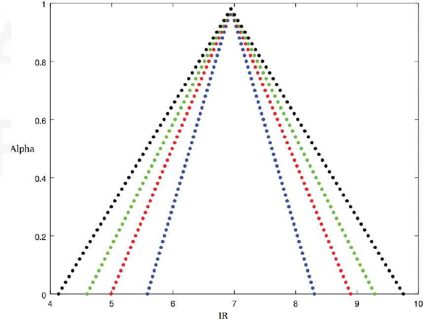
The method provided in (18) is not determined in terms of α-cuts, in contrast to the methods presented in the literature [9–11,14]. Moreover, Proposition 4 reveals that Yk+1 is a fuzzy number for every k. Consequently, the verification of the Negoita–Ralescu characterization theorem is not necessary in order to guarantee this fact. Hence, Figures 8–10 illustrate the statement (i) of Remark 1.
Figure 8
Numerical solutions to the chemical decay reaction given in Equation (19), at time t=3. The blue, red, green and black dots represent the fuzzy numbers that were obtained for γ=0, γ=0.5, γ=0.75, and γ=1, respectively.
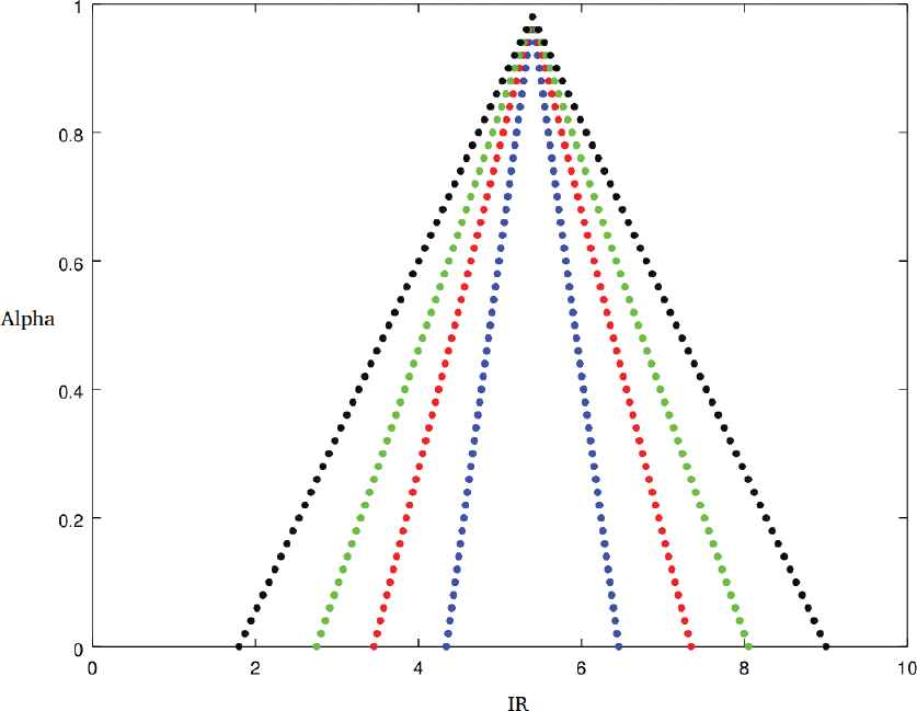
Figure 9
Numerical solutions to the chemical decay reaction given in Equation (19), at time t=5. The blue, red, green and black dots represent the fuzzy numbers that were obtained for γ=0, γ=0.5, γ=0.75, and γ=1, respectively.
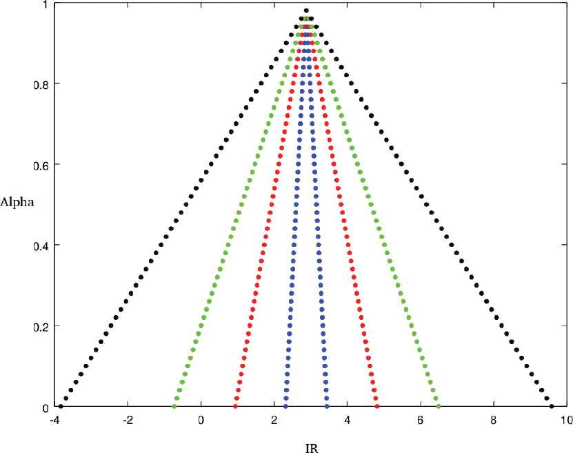
Figure 10
Numerical solutions to the decay chemical reaction given in Equation (19), at time t=10. The blue, red, green and black dots represent the fuzzy numbers that were obtained for γ=0, γ=0.5, γ=0.75, and γ=1, respectively.
Item (ii) of Remark 1 requires that Yik and hfi(tk,Y1k,…,Ynk) must be interactive with respect to some joint possibility distribution for every k. Otherwise, interactive arithmetic cannot be employed. Note that the family Jγc has no restrictions and can be used for any pair of fuzzy numbers, in contrast to the joint possibility distribution JL. Thus, the method (18) can be always used for the family Jγc.
When using joint possibility distributions, the arithmetic operations in numerical methods must be established before computing the iterations, meaning that the joint possibility distribution must be predetermined. Thus, Item (iii) of Remark 1 ensures that all arithmetic operations should be based on joint possibility distributions, that is, the arithmetic operations must be interactive.
Recall that there are several methods in the literature that uses the standard sum and the generalized Hukuhara difference (−gH) [33] in the same numerical method. This is not consistent since the gH-difference is an interactive arithmetic operation [31], in contrast to the standard sum. In other words, Item (iii) of Remark 1 establishes that if one considers the gH-difference in the numerical method, then the sum under consideration must be interactive, for example, +0.
The next section presents a discussion about the computational effort for generating the numerical solution proposed by Wasques et al. [8].
5. COMPUTATIONAL COST OF THE NUMERICAL SOLUTION
In the oscillating chemical reaction problem addressed in Section 6, the number of operations to compute
Yik+1=Yik+γhf(tk,Y1k,…,Ynk).
depends on the number of arithmetic operations present in the function f. In what follows, we assume that [Yi0]1={yi}, yi∈ℝ, for all i=1,…,n.
In order to estimate the computational cost of this numerical solution, we must provide the computational effort to perform each arithmetic operation A1⊗γA2. From the proof of Item (b) of Theorem 2 in [25], we have that [Jγ]α is a connected and compact set of ℝ2 for all α,γ∈[0,1]. Thus, by Nguyen's theorem, we have [A1⊗γA2]α=⊗([Jγ]α), for all α∈[0,1], where
[Jγ]α=⋃i=12⋃β∈[α,1]Wi,β,
with Wi,β={(x1,x2):xi∈Rβi,x3−i∈Li(xi,β,γ)}.
Consequently, we obtain
⊗([Jγ]α)=⋃i=12⋃β∈[α,1]⊗(Wi,β),
which implies that we have to compute the minimal and maximal values of ⊗(Wi,β), in order to calculate the α-cuts of A1⊗γA2.
Let us analyze the set Wi,β. To this end, consider the following partition of [0,1]
P=α0=0,α1=1p,…,αp−1=p−1p,αp=1.
For convenience, also consider the following partition for [αi,1]
Q=αi=ip,αi+1=i+1p,…,αp=1,
for each αi∈P with i∈0,1,…,p.
Hence, for each βj∈Q there are seven operations to compute the function g∧i(z,β) and five operations to compute the function g∨i(z,β), since these functions can be evaluated as follows:
Consequently, to construct the interval [l,r] given in the definition of Jγ(14), there are required nineteen operations, seven for g∧i, five for g∨i, four for the function vi, two for the left side of the interval [l,r] and one for the right side.
Since the intersection of two intervals can be given by taking the maximum value between the left endpoints and the minimum value between the right endpoints, the construction of the interval Li(z,β,γ) requires the total of twenty one operations.
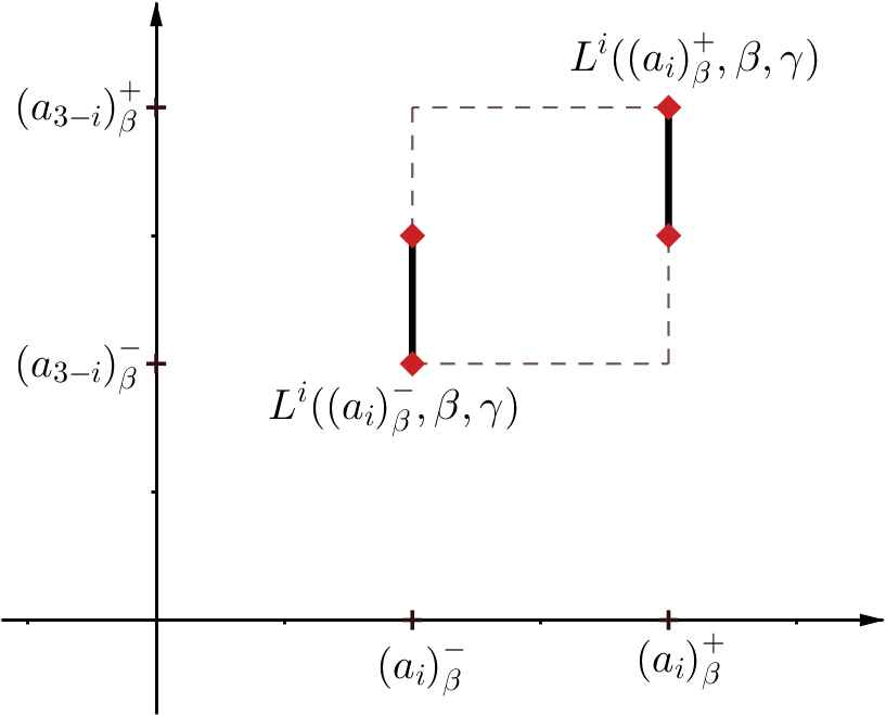
Each xi∈Rβi is associated to the interval Li(xi,β,γ). Figure 11 illustrates this situation. Thus, the minimal and maximal values of ⊗(Wi,β) occur for four pairs (x1,x2) (see Figure 11). This implies that six more operations are required at this step.
Figure 11
The black segments represent the intervals Li(xi,β,γ), where xi∈Rβi. The red diamonds represent the pairs (x1,x2) of the set Wi,β that may occur the miminum and maximum of ⊗(Wi,β).
Therefore, for each βj∈Q we must compute twenty seven operations, implying a cost of 27(p−i+1) operations, for each αi∈P. Consequently, the computational complexity is O(p2) in each iteration. This result is established in Theorem 5. For the particular case where γ=1, one can prove that the minimum and maximum of ⊗([Jγ]α) is obtained over W1,α∪W2,α. In this case, we have only 27 operations for each βj∈Q, implying a computational effort of O(Kp). This last result was expected, as the standard arithmetic is obtained when γ=1 and, therefore, [A1⊗1A2]α is given in terms of interval arithmetic of the corresponding α-cuts of A1 and A2. However, in general, numerical solutions based on standard arithmetic have increasing width over time.
Theorem 5.
IfP=α0,α1,…,αp−1,αp, whereαi=ipfor alli=0,1,…,p, is a discretized version of[0,1], then the computation of the fuzzy numbersY1k+1,….,Ynk+1via (18) requiresO(p2)operations for each iterationk.
Theorem 5 reveals that the application of (18) in a discretized setting in P, where |P|=p+1, leads to a quadratic computational complexity O(p2) for each iteration k∈{1,…,K}. Therefore, determinig the numerical solution via (18) requires O(Kp2) operations whereas the classical Euler method requires O(p) operations in the aforementioned discretized setting.
In comparison to other methods in the literature, Ahmadian et al. [10] proposed a numerical solution based on the Runge–Kutta method, which requires only three function evaluations for each iteration. This leads to a reduction in the computational cost for numerical solutions to FDEs, since the problem is reduced to a crisp analysis for each α∈[0,1]. However, this procedure (and many others) only guarantees that the α-cuts of the numerical solution are intervals. Thus, in order to ensure that they produce a fuzzy solution, the conditions of Negoita–Ralescu theorem must be satisfied. Otherwise, these methods may not yield a fuzzy solution, because it does not necessarily produce a fuzzy number at every instant of time, as we point out in Remark 1. On the other hand, our proposed method guarantees that the numerical solution provides a fuzzy number in each iteration, but requiring a computational cost of quadratic order.
Section 6 presents an application on a particular type of chemical reaction, called oscillating chemical reaction. This application illustrates the proposed method, considering uncertain initial concentrations given by fuzzy numbers.
6. APPLICATION TO THE LOTKA–VOLTERRA MODEL OF OSCILLATING CHEMICAL REACTIONS
It is well known that some chemical reactions may be oscillating in time or space [4], meaning that the concentrations of the reagents and products are changing with time in a periodical way [34].
The trajectory of an oscillating chemical reaction depends on its initial condition, influencing the concentrations of the products. Hence, oscillating chemical reactions may exhibit chaotic behavior [35]. This type of reaction is used to describe several processes in chemistry [36,37].
This paper considers a particular example of oscillating chemical reaction called Lotka–Volterra model. The focus is to provide a numerical solution for the system given by (3) in order to simulate the behavior of this reaction in the case where the initial concentrations are uncertain, illustrating the effects that interactivity may produce in the numerical solutions.
Having said that, let the initial conditions [A0], [X0], [Y0] and [B0] be given by fuzzy numbers. Hence the addition given by Equations (4) and (5) must be adapted to fuzzy numbers. The chosen addition is the one obtained via Jγc (see (10)).
Consequently, the sum operation depends on the values of γ∈[0,1]. Thus, Equation (4) becomes
[A(t)]+γ[X(t)]+γ[Y(t)]+0[B(t)]=k,(21)
where the last sum of (21) is given by +0 in order to guarantee that k∈ℝ.
In particular,
([A0]+γ[X0]+γ[Y0])+0[B0]=k.(22)
Thus, it follows that
[B(t)]=k−0[A(t)]+γ[X(t)]+γ[Y(t)],(23)
for all t∈[0,T].
Therefore, from Equation (23), one concludes that it is only necessary to solve the first three equations of (3).
The numerical solution for this problem is based on the method provided in Section 4. Hence the fuzzy numerical solution is given by
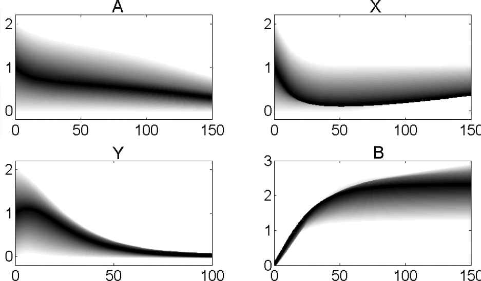
Figures 12–14 visualize simulations for three different “levels” of interactivity, that is, γ=0, γ=0.5 and γ=0.75, using the following parameters: h=0.125, k1=0.03, k2=0.09, k3=0.06 and [A0]=[X0]=[Y0]=(0;1;2).
Figure 12
Numerical solution for γ=0. The approximate fuzzy solutions at each instant of time are represented using shades of gray. High values of an approximate fuzzy solution at time t are depicted in dark gray while low values are depicted in light gray. Black and white correspond respectively to 1 and 0.
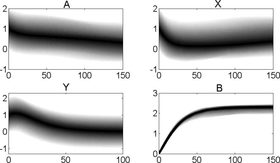
Figure 13
Numerical solution for γ=0.5.
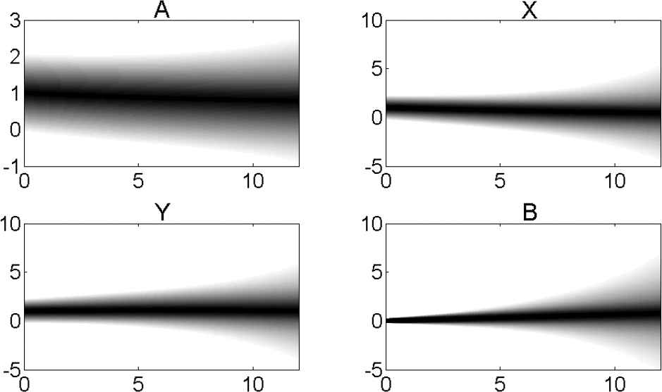
Figure 14
Numerical solution for γ=0.75.
Note that for different values of γ, one obtains different final products. This fact is associated with the interactive arithmetic that is based on the family of the joint possibility distribution Jγc [8].
Figure 12 illustrates that the highest level of interactivity (γ=0) yields decreasing width for the reagents A, X and Y over time. However the width of the final product increases initially and thereafter has few variations.
Figure 13 reveals that for γ=0.5 (medium level of interactivity) the width of A, X and Y has few variations. The width of the product also has few variations but always with a width that is smaller than the width of the fuzzy solution provided by γ=0.
Even though for γ=0.5 the reagents have a greater uncertainty than for γ=0, the uncertainty in the final product is smaller. Thus, in this sense, the solution via J0.5 may describe this final product in a more precise way.
For γ=0.75 one expects that the uncertainty increases over time, since the value of γ is closer to 1 [8]. This fact is corroborated by Figure 14.
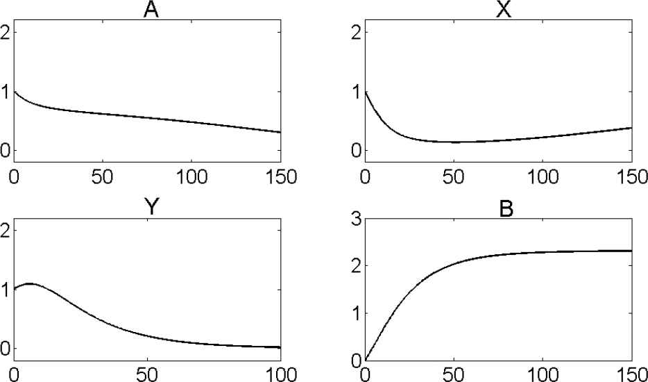
Figure 15 illustrates the deterministic solution of the system (3) with initial values [a0]=[x0]=[y0]=1.
Figure 15
The deterministic numerical solution.
On the one hand, note that the joint possibility distributions J0 and J0.5 produce solutions qualitatively similar to the deterministic case (see Figures 15, 12, and 13). On the other hand, the joint possibility distribution J0.75 produces a numerical solution with so much uncertainty that the final result does not resemble (qualitatively) the deterministic solution.
Hence, in the context of fuzzy set theory, the relationship of interactivity (as well as the level of interactivity given by γ) influences the final product. This means that from the perspective of chemistry, it is possible to control the uncertainty of the final product concentration, even if there exists an uncertainty in the quantities and/or concentration of the reagents.
Recall that for other types of chemical reaction, such as reversible ones [38], the numerical solution for γ=0 may describe the evolution of the reaction more precisely than other values of γ∈(0,1].
7. CONCLUDING REMARKS
This work studies chemical reactions from the fuzzy set theory perspective. More precisely, we provide a numerical solution for chemical reaction models described by a system of differential equations. The initial conditions of this system are given by interactive fuzzy numbers, in order to take possible uncertainties in the reagent concentrations into account.
The relationship of interactivity models the dependence of the final product on the concentration of the initial and intermediary reagents. It was verified that the interactivity interferes with the width of the fuzzy numerical solution which describes the uncertainty of the reagents and the final product concentrations.
This paper shows that, when using numerical methods, the arithmetic operations must be interactive. This means that it is not consistent to use the standard sum and the Hukuhara (and its generalizations) difference in the same method since the Hukuhara difference is an interactive arithmetic operation, in contrast to the standard sum [31].
The numerical methods proposed in the literature are given in terms of α-cuts and the simulations are performed using interval arithmetic. This procedure does not guarantee that the numerical solution produces a fuzzy number at each instant of time, which is necessary since the analytical solution must be a fuzzy function. This paper reveals the power of the proposed method since the fuzzy solution yields a fuzzy number at each instant of time (see Remark 1).
We also investigated the computational effort of proposed method. Under some conditions, we concluded that the computational complexity of the numerical method is quadratic, as established by Theorem 5. However, the proposed numerical method has the advantage of yielding a fuzzy number at every iteration. This differs from many numerical methods which associate a given FDE to a family of pairs of classical differential equations whose solutions could represent the endpoint functions of the α-cuts of a fuzzy solution. However, in general, a drawback of this type of approach lies in the fact there is no guarantee that the requirements of Negoita–Ralescu theorem is satisfied at every instant. In other words, there is no guarantee that the obtained solution describes a fuzzy number at every instant.
We applied our method to the Lotka–Volterra model of oscillating chemical reactions and verified that different types of interactivity yield different solutions for this problem. The value of γ=0.5 produced a solution with less uncertainty in the final product than the numerical solution for γ=0, in contrast to what occurs for reversible chemical reactions [38].
Instead of a FIVP where the derivative is obtained by a fuzzy process [7,39], we use a numerical method for FIVPs to observe how the relationship of interactivity acts in the chemical reagents when the initial conditions were given by interactive fuzzy numbers.
CONFLICTS OF INTEREST
The authors declare that they have no known competing financial interests or personal relationships that could have appeared to influence the work reported in this paper.
AUTHORS' CONTRIBUTIONS
Vinícius F. Wasques: Formal analysis, Validation, Investigation, Writing - Original Draft. Estevão Esmi: Formal analysis, Conceptualization, Investigation, Writing - Review and Editing, Supervision, Funding acquisition. Laécio C. Barros: Formal analysis, Investigation, Conceptualization, Writing - Review and Editing, Supervision, Funding acquisition. Peter Sussner: Conceptualization, Investigation, Writing - Review & Editing, Funding acquisition.
ACKNOWLEDGMENTS
The authors are grateful for the support of CNPq under grant nos. 306546/2017-5 and 313145/2017-2, and FAPESP under grant nos. 2016/26040-7 and 2018/13657-1.
REFERENCES
1.G.F. Froment, K.B. Bischoff, and J. Wilde, Chemical Reactor Analysis and Design, Random House, New York, NY, USA, 1988. ISBN: 978-0-470-56541-4
2.P. Flowers, K. Theopold, R. Langley, and W.R. Robinson, Chemistry, OpenStax, Houston, Texas, TX, USA, 2015. ISBN-10: 1-947172-62-X
30.V.F. Wasques, N.J.B. Pinto, E. Esmi, and L.C. Barros, Consistence of interactive fuzzy initial conditions, in Annual Conference of the North American Fuzzy Information processing Society NAFIPS (Redmond, United States), 2020.
38.V.F. Wasques, E. Esmi, L.C. Barros, and F. Santo Pedro, Numerical solution for reversible chemical reaction models with interactive fuzzy initial conditions, in Annual Conference of the North American Fuzzy Information processing Society NAFIPS (Redmond, United States), 2020.
TY  - JOUR
AU  - Vinícius F. Wasques
AU  - Estevão Esmi
AU  - Laécio C. Barros
AU  - Peter Sussner
PY  - 2020
DA  - 2020/09/24
TI  - Numerical Solution for Fuzzy Initial Value Problems via Interactive Arithmetic: Application to Chemical Reactions
JO  - International Journal of Computational Intelligence Systems
SP  - 1517
EP  - 1529
VL  - 13
IS  - 1
SN  - 1875-6883
UR  - https://doi.org/10.2991/ijcis.d.200916.001
DO  - 10.2991/ijcis.d.200916.001
ID  - Wasques2020
ER  -

 , Estevão Esmi2, Laécio C. Barros2, Peter Sussner2,