
Multiple Bipolar Fuzzy Measures: An Application to Community Detection Problems for Networks with Additional Information

- DOI
- 10.2991/ijcis.d.201012.001How to use a DOI?
- Keywords
- Networks; Community detection; Bipolar fuzzy graph; Extended bipolar fuzzy graphs; Multiple bipolar fuzzy graph; Extended multiple bipolar fuzzy graphs; Louvain algorithm
- Abstract
In this paper we introduce the concept of multiple bipolar fuzzy measures as a generalization of a bipolar fuzzy measure. We also propose a new definition of a group, which is based on the multidimensional bipolar fuzzy relations of its elements. Taking into account this information, we provide a novel procedure (based on the well-known Louvain algorithm) to deal with community detection problems. This new method considers the multidimensional bipolar information provided by multiple bipolar fuzzy measures, as well as the information provided by a graph. We also give some detailed computational tests, obtained from the application of this algorithm in several benchmark models.
- Copyright
- © 2020 The Authors. Published by Atlantis Press B.V.
- Open Access
- This is an open access article distributed under the CC BY-NC 4.0 license (http://creativecommons.org/licenses/by-nc/4.0/).
1. INTRODUCTION
In general, relations, communication or even feelings among humans, have two aspects, the positive and the negative. The first one expresses possible or permitted evidences which provide satisfaction. On the contrary, the negative aspect represents impossible relations or situations which are unacceptable or not permitted, and provide dissatisfaction [1].
When some message arrives to human consciousness, the mind automatically assigns to it negative and positive evidences. Being able to deal in this way with the information, while simultaneously considering positive and negative evidences, humans are capable of representing and handling with complex situations and scenarios connected to sensations, ambivalence, conflicts, or interests [2]. This peculiar manner of managing information has its basis on the idea of bipolarity, which was originally a psychological concept [3].
In this work we take into account these considerations, adding them in the field of graphs or networks, which are one of the most important fields in which clustering methods are applied. Given a finite set of objects, graphs are used to model and visualize the relations or connections among its elements. The complexity of these problems grows almost exponentially with the consideration of models requiring hundreds or thousands of individuals and edges, so it becomes very more important to build robust and effective systems to choose the most appropriate algorithms for defining blocks.
Communities can be understood as groups of related individuals in social networks [4], biochemical pathways in metabolic networks [5], or even sets of Web pages dealing with the same topic [6]. Apart from their wide range of applications, communities can be used to visualize how the society works. A community structure can also be used to find groups of elements depending on their relations. As far as possible, we assume that a group should be composed of elements between which there is some affinity, trying to keep separate those elements between which there is some discrepancy.
In this paper, we follow the philosophy introduced in [7], which consists in considering some bipolar additional information independent of the topology of the graph for community searching. Doubtlessly, the connections among the individuals, modeled by the edges of the graph, should be the main factor in the search of a cluster structure. However, it would be reasonable to consider some additional information apart from that provided by the structure of the graph, in order to extend the notion of community. Moreover, this double perception of the information may be given by several sources. Here lies the importance of working with multiple bipolar fuzzy measures.
Let us show an example with
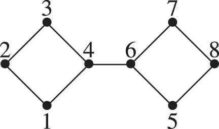
Example. Graph with 8 nodes.
According to our best knowledge, this way to manage the additional information with a double perception in a multiple case, is an approach which has never been deeply studied. Recent studies have dealt with the problem of incorporating some additional information when finding a cluster structure in a graph [8–11]. A preliminary work focused on improving the community detection problem by incorporating the use of fuzzy measures, was published in [12]. This proposal is based on the consideration of fuzzy measures defining affinity relations, so that we know which nodes should be in the same cluster.
Later, in [7], it was proposed the use of a bipolar fuzzy measure to find communities in a network in a more realistic way. Hence, considering this bipolar fuzzy measure (in a unidimensional case), not only the positive information, but also the negative one is analyzed to define clustering structures.
Now we come up with the use of multiple bipolar fuzzy measures, which allow us to approach complex scenarios that cannot be modeled with those tools exploited in previous works. In this background, we know not only which elements should be in the same group because of their affinity, but also which ones should be separated due to their discrepancy. This approach is somewhat similar to intuitionistic fuzzy cognitive maps (FCMs) [13,14] (in a multidimensional scale), that describe the connections between nodes by membership/nonmembership values.
Then, in this work we propose an extension of the Louvain algorithm [15] which can consider two types of input information. One is about the direct connections between the nodes, given by the edges of the graph. It is used to find “possible” clusters. The other, which could be also the edges of the graph or even an independent information, is used to search the maximum of modularity. This new approach, called Duo Louvain, is formalized in Algorithm 2. Then, we propose a particular application of Duo Louvain Algorithm, named Multiple Bipolar Duo Louvain Algorithm, for searching community structures in extended multiple bipolar fuzzy graphs. It is formalized in Algorithm 3. There, in a multidimensional case, we develop a way to manage bipolar information which shows us which nodes should be separated, and which ones should remain together.
We test the “goodness” of our proposal with the use of different benchmark models [16], in combination with the calculation of the Normalized Mutual Information (
The remainder of the paper is organized as follows: In Section 2 we describe the concepts we will use along the paper, including the definition of extended bipolar fuzzy graphs, the bipolar weighted multi-graph associated with a bipolar fuzzy measure, and some definitions of aggregation operators (AOs). In Section 3, we introduce some key concepts: the extended multiple bipolar fuzzy graph and the bipolar weighted multi-graph associated with multiple bipolar fuzzy measures. In this section we also describe the aggregation process proposed to deal with this complex information. Section 4 is devoted to the Louvain algorithm, including a detailed explanation about its performance in Subsection 4.1, and a modification of it to deal with community detection problems based on multiple bipolar fuzzy measures, in Subsection 4.2. We test the performance of our proposal with some computational results in Section 5. To finish the paper, we provide some conclusions and final remarks in Section 6.
2. PRELIMINARIES
2.1. AOs and Other Functions
AOs [18] are one of the hottest disciplines in information sciences. AO appear in a natural way when the soft information has to be aggregated. At the beginning, AO were defined to aggregate values from membership functions associated with fuzzy sets [19]. AOs, also known as aggregation functions, are a key concept for the development of this paper.
Definition 1.
Aggregation Function [18]. The function
Let us note that aggregation functions are usually classified into four different classes, by means of their point-wise comparison to the maximum and minimum operators. These classes are as follows:
Disjunctive aggregation function: an aggregation function
Conjunctive aggregation function: an aggregation function
Averaging aggregation function: an aggregation function
Mixed aggregation function: an aggregation function
Finally, let us define the negation operator that will be used later in this paper.
Definition 2.
Negation Operator [20]. Given a partial ordered set
2.2. Fuzzy Graphs, Bipolar Fuzzy Graphs, and Weighted Graphs Associated with Fuzzy Measures
Let the pair
Fuzzy graphs, introduced by Rosenfeld [21], depict other type of networks with a wider scope. These graphs are really useful for modeling situations in which there is some uncertainty. Fuzzy graphs are based on the fuzzy relations among the individuals [19], representing the degree of these relations. Here we provide a formal definition of fuzzy graphs.
Definition 3.
Fuzzy graph [21]. Let
Assuming that the vertex set
Definition 4.
Crisp graph with fuzzy edges [22]. Let
Let us note that a pair of nodes which are not adjacent in the crisp graph
Definition 5.
Fuzzy measure [23]. Let be the finite set
Hence, an extended fuzzy graph is a graph together with a fuzzy measure. Formally:
Definition 6.
Extended fuzzy graph [12]. Let
Thus far, we have just considered fuzzy measures with an individual interpretation. Now, let us extend the application framework by considering bipolar fuzzy measures [24].
Definition 7.
Bipolar Fuzzy Measure [24] Let
To adapt the interpretation of
Definition 8.
Extended bipolar fuzzy graph [7]. Let be the graph
2.3. Defining Groups from Fuzzy Measures: The Associated Weighted Graph
Given a fuzzy measure
There exist different ways to build a weighted graph from a fuzzy measure. In the proposal done in [12], the definition of this weighted graph was based on the Shapley value related to a fuzzy measure.
Definition 9.
Shapley value[27]. Let be the fuzzy measure
The weighted graph associated with a fuzzy measure [12] is that whose adjacency matrix is defined as
Then, for each pair of nodes
Taking into account that a bipolar fuzzy measure,
Definition 10.
Bipolar weighted multi-graph associated with a bipolar fuzzy measure. Let
3. MULTIPLE BIPOLAR FUZZY MEASURES IN GRAPHS
As happen in any statistical real problem, more than one variable is needed to represent in a more natural way the reality. Objects cannot be described just by one variable; there are even many situations in which the similarity (or dissimilarity) between objects depends on more than one criterion. Considering this fact, it is fair to assume that the fuzzy measures that represent the synergies between objects that we are going to cluster, could also not be unidimensional. In addition to this fact, as it was pointed in [7], bipolarity appears in a natural way: there are some capacities that represent the synergies or similarity between objects, but there are also others that represent the dissimilarity or negative synergies (antagonism). Considering all this, in this section we propose a generalization of the extended bipolar fuzzy graph into a multidimensional case and we propose an aggregation process to deal with this complex information.
Definition 11.
Extended multiple bipolar fuzzy graph. Let
Once the extended multiple bipolar fuzzy graph is defined, we propose a five-step methodology to transform the information provided by the extended multiple bipolar fuzzy graph, for further combination of this transformed information with a community detection algorithm. The process is quite similar to that followed in Definition 10, but in this case, we have to manage
The first step is to summarize the information given by each bipolar fuzzy measure into two matrices. Particularly, for the bipolar fuzzy measure
Definition 12.
Bipolar weighted multi-graph associated with multiple bipolar fuzzy measures. Let
This new concept (bipolar weighted multi-graph associated with multiple bipolar fuzzy measures) summarizes (particularly for our clustering purpose) the information provided by the
Step 1: Built bipolar weighted multi-graph. Given a multiple extended bipolar fuzzy graph, the adjacency matrices
Step 2: Aggregating negative information. In this case, we first aggregate matrices
wherebeingStep 3: Aggregating positive information. In a similar way, we aggregate the matrices
wherebeingStep 4: Transforming negative information. Let us note that matrices
Step 5: Final aggregation. Finally, we combine the information provide by
wherebeing
Remark 1.
Note that previous process involves three different classes of AOs: one for positive information, other for the negative one, and finally, another for combining the positive and negative information. In this paper we present the aggregation problem/process in a general way since any AO could be used. We think that the aggregation should be strongly dependent on the real problem that you are dealing with.
In the unidimensional case, we only used this last class of AO, so just three notions of group were contemplated:
If
If
If
The problem becomes more complex when there are several information sources, with positive and negative meanings, which have to be aggregated. If we force to the AOs
In the computational results section, we have used average AOs for
4. THE MULTIPLE BIPOLAR DUO LOUVAIN ALGORITHM
This section is based on one of the most popular algorithms in community detection framework: the Louvain algorithm [15]. Hence, first we explain the main points of this method, to provide a clear vision of its performance. Then, we propose a modification of it that allows us to deal with problems in which there is some additional information. Particularly, we propose an application of this modification to deal with community detection problems based on multiple bipolar fuzzy measures.
4.1. Louvain Algorithm
In last decades, the interest of many researchers has been focused on community detection problem, so many effective method have been proposed in this field. In 2008, Blondel et al. introduced one of the most popular algorithms in networks literature: the Louvain algorithm [15]. Based on local moving heuristic and modularity optimization [29], this algorithm, widely used due to its speed and effectiveness, provides a nonhierarchical partition, obtained in a multi-phase process. Two concepts are essential on this process: the modularity of a partition and the variation of modularity obtained when moving node
Definition 13.
Modularity
Definition 14.
Variation of modularity
Now we show a sketch about Louvain performance, which is divided into two phases.
Phase 1. At the beginning, each node of the graph defines in itself an isolated community. For each node
This process is sequentially and repeatedly applied for the entire set of nodes with random order (in fact, one node could be analyzed several times), until a local maximum of the modularity is reached. Then, the first phase ends.
Phase 2. Considering the communities defined in the first phase as nodes, which are called supervertices [31], the second phase starts with the construction of a new network whose nodes are these supervertices. Two supervertices are connected if there is at least one edge among them, i.e., there is at least one node in one supervertice connected with one node in the other supervertice. To calculate the weight of each supervertice, we have to sum the weight of the edges between the communities found in the original graph. Furthermore, there could be self-loops, given by the edges between nodes which are in the same supervertice. Once the new network is defined, the next part of this phase consists on the application of the first phase, considering the new graph.
Both phases are iteratively repeated while there are changes in modularity, until a maximum of modularity is achieved. In Algorithm 1 we provide a sketch of the performance of this algorithm, by means of its pseudocode.
Note that, because of its order dependence, the solution obtained with the Louvain algorithm is not unique [32]. Usually, several outputs of the same networks are analyzed, considering random reshuffling of the order in which the nodes are evaluated [33].
Algorithm 1: Louvain input = A P
1: Phase 1.
2:
3: Let each node of the graph be an isolated community
4: While There is some change in modularity optimization
5: According to the order given by
6: Calculate
7: Let
8: If
9: Move node
10: Else
11:
12: End while
13: Phase 1 Ends
14: Phase 2
15:
16: While there is some change, apply the Louvain Algorithm, considering matrix
17: Phase 2 Ends
4.2. Louvain Algorithm Over Extended Multiple Bipolar Fuzzy Graphs
In this section we explain a modification of the Louvain algorithm [15] to deal with situations in which there is some additional information about the relations among the nodes, given by multiple bipolar fuzzy measures which are independent of the structure of the graph.
First, we propose a new concept of group which is based on the notion of extended multiple bipolar fuzzy graph (see Definition 11). Hence, let
On the other hand, to carry on with community detection problems with additional information given by multiple bipolar fuzzy measures, let us propose an alternative vision of the Louvain algorithm. We want to differentiate two input parameters in this algorithm. One, the matrix used to find “possible” clusters. It provides information about the edges between the nodes. The other is the matrix used to calculate the modularity optimization for a possible local moving. Obviously, the Louvain algorithm considers the same matrix for both purposes (the adjacency matrix of the graph).
Now we define an algorithm based on this alternative vision of the Louvain algorithm. Let
Let us remark that the complexity of Duo Louvain algorithm is exactly the same as the complexity of the Louvain algorithm.
Then we explain how to apply the proposed algorithm when solving community detection problems based on multiple bipolar fuzzy measures. Let
To find communities in
Algorithm 2: Duo Louvain input = A , ℳ P
1: Phase 1.
2:
3: Let each node of the graph be an isolated community
4: While There is some change in modularity optimization
5: According to the order given by
6: Calculate
7: Let
8: If
9: Move node
10: Else
11:
12: End while
13: Phase 1 Ends
14: Phase 2
15:
16:
17: While there is some change, apply the Duo Louvain Algorithm, considering matrices
18: Phase 2 Ends
We will explain with a pseudocode this particular application of Algorithm 2 for solving community detection problems based on multiple bipolar fuzzy measures. For each bipolar fuzzy measure
Algorithm 3: Multiple Bipolar Duo Louvain input = A , μ b 1 , … , μ b s P
1: for
2:
3:
4: end for
5:
6:
7:
8:
9:
10: Apply Duo Louvain
Regarding the calculation of Shapley value, it has an exponential complexity, which can be partially solved with sampling techniques [38,39]. However, we want to remark that when additive fuzzy measures are considered, the exact calculation of this value is immediate [12]. Hence, in this context, the complexity of Algorithm 3 is exactly the same as the Louvain algorithm.
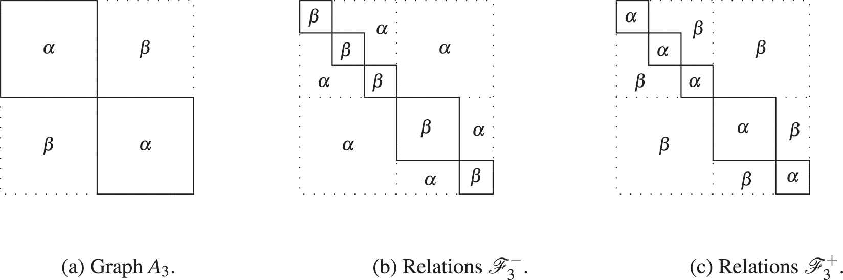
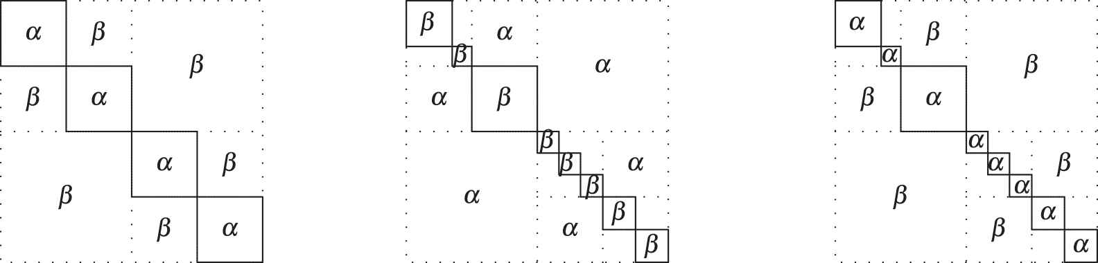
Let us recall the example proposed in the Introduction. Now we show that the Algorithm 3, Multiple Bipolar Duo Louvain finds the communities which seemed to be logical when considering the affinity/discrepancy relations among the individuals.
Example 1.
Let
Adjacency matrix 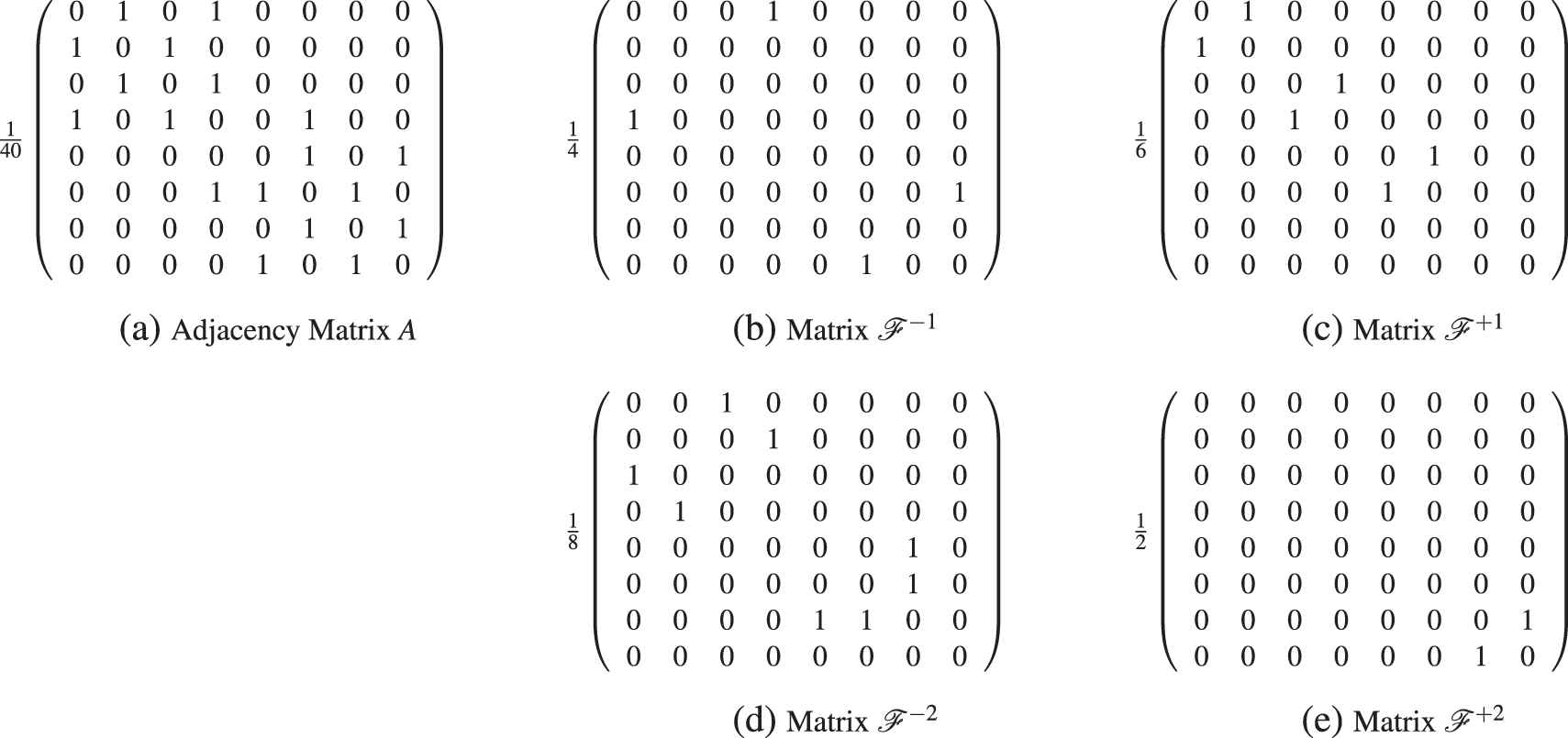
We calculate
5. COMPUTATIONAL RESULTS
In this section we provide some computational results in order to test the effectiveness of the Algorithm 2, with the particular application given in Algorithm 3 used to solve community detection problems based on multiple bipolar fuzzy measures. To carry on with it, we work with benchmark models [16]. Here we propose four different “standard” or “gold” structures. The objective is to quantify, by means of the
Definition 15.
Normalized Mutual Information
Then, the
According to Equation (5), the
5.1. Benchmark Graphs
When a new method is proposed, one of the most important issues is its comparison with the existing work, in order to test if the new proposal is at least as good as the old ones. One crucial point when testing clustering methods is about which evidence or characteristic should be analyzed: not only the complexity or speed of the method should be considered but also the goodness of the results should be measured. The issue is that each method has its own characteristics and peculiarities, even the output might not be comparable. So, in this work we focus the test on benchmarking. In [40], Bader et al. said “Benchmarking refers to a repeatable performance evaluation as a means to compare somebody's work to the state of the art in the respective field.”
Then, in this paper we artificially build benchmark graphs. These are synthetic graphs generated with an embedded cluster structure. This structure is assumed to be a “standard” or gold partition, and the main point is to analyze the ability of an algorithm to find it. We quantify this ability with the calculation of the
To generate these benchmark models, we assume that both the expected degree,
5.2. Results
In this subsection we generate four different benchmark graphs, based on the idea proposed in [4], as it is explained in the previous section. We work in a broad context, considering also asymmetric structures. Each model, representing an extended multiple bipolar fuzzy graph
Both the adjacency matrix
| Label | ||
|---|---|---|
| 1 | 0.45 | 0.016 |
| 2 | 0.4 | 0.033 |
| 3 | 0.35 | 0.05 |
| 4 | 0.325 | 0.058 |
| 5 | 0.3 | 0.066 |
| 6 | 0.275 | 0.075 |
| 7 | 0.25 | 0.083 |
| 8 | 0.225 | 0.091 |
| 9 | 0.2 | 0.1 |
Benchmark parameters.
In all the cases showed in this section, matrices
For each combination of the parameters
| NMI | Relations Value 1 | Relations Value 2 | Relations Value 3 | Relations Value 4 | Relations Value 5 | Relations Value 6 | Relations Value 7 | Relations Value 8 | Relations Value 9 |
|---|---|---|---|---|---|---|---|---|---|
| Graph Value 1 | 1 | 1 | 1 | 1 | 1 | 0.9999 | 0.9985 | 0.9667 | 0.8159 |
| Graph Value 2 | 1 | 1 | 1 | 1 | 1 | 1 | 0.9980 | 0.9712 | 0.8115 |
| Graph Value 3 | 1 | 1 | 1 | 1 | 1 | 1 | 0.9983 | 0.9597 | 0.8056 |
| Graph Value 4 | 1 | 1 | 1 | 1 | 1 | 1 | 0.9970 | 0.9964 | 0.8029 |
| Graph Value 5 | 1 | 1 | 1 | 1 | 1 | 1 | 0.9983 | 0.9640 | 0.8091 |
| Graph Value 6 | 1 | 1 | 1 | 1 | 1 | 1 | 0.9987 | 0.9555 | 0.8087 |
| Graph Value 7 | 1 | 1 | 1 | 1 | 1 | 1 | 0.9978 | 0.9686 | 0.8004 |
| Graph Value 8 | 1 | 1 | 1 | 1 | 1 | 1 | 0.9964 | 0.9591 | 0.8067 |
| Graph Value 9 | 1 | 1 | 1 | 1 | 1 | 1 | 0.9978 | 0.9683 | 0.8091 |
| NMI | Relations Value 1 | Relations Value 2 | Relations Value 3 | Relations Value 4 | Relations Value 5 | Relations Value 6 | Relations Value 7 | Relations Value 8 | Relations Value 9 |
|---|---|---|---|---|---|---|---|---|---|
| Graph Value 1 | 1 | 1 | 1 | 1 | 0.9978 | 0.9891 | 0.9703 | 0.9814 | 0.9939 |
| Graph Value 2 | 1 | 1 | 1 | 1 | 0.9995 | 0.9900 | 0.9801 | 0.9883 | 0.9999 |
| Graph Value 3 | 1 | 1 | 1 | 1 | 0.9981 | 0.9943 | 0.9935 | 0.9919 | 0.9937 |
| Graph Value 4 | 1 | 1 | 1 | 1 | 0.9991 | 0.9948 | 0.9921 | 0.9907 | 0.9997 |
| Graph Value 5 | 1 | 1 | 1 | 1 | 0.9992 | 0.9929 | 0.9877 | 0.9701 | 0.9950 |
| Graph Value 6 | 0.9999 | 1 | 1 | 1 | 0.9998 | 0.9935 | 0.9849 | 0.9882 | 0.9903 |
| Graph Value 7 | 0.9999 | 1 | 1 | 1 | 0.9995 | 0.9981 | 0.9928 | 0.9935 | 0.9917 |
| Graph Value 8 | 0.9998 | 0.9998 | 1 | 1 | 1 | 0.9971 | 0.9950 | 0.9878 | 0.9821 |
| Graph Value 9 | 0.9991 | 0.9997 | 0.9991 | 0.9997 | 0.9994 | 0.9991 | 0.9979 | 0.9899 | 0.9895 |
| NMI | Relations Value 1 | Relations Value 2 | Relations Value 3 | Relations Value 4 | Relations Value 5 | Relations Value 6 | Relations Value 7 | Relations Value 8 | Relations Value 9 |
|---|---|---|---|---|---|---|---|---|---|
| Graph Value 1 | 1 | 1 | 1 | 1 | 0.9995 | 0.9929 | 0.9680 | 0.9145 | 0.8431 |
| Graph Value 2 | 1 | 1 | 1 | 1 | 0.9989 | 0.9916 | 0.9608 | 0.9116 | 0.8405 |
| Graph Value 3 | 1 | 1 | 1 | 1 | 0.9984 | 0.9935 | 0.9627 | 0.9067 | 0.8418 |
| Graph Value 4 | 1 | 1 | 0.9997 | 0.9997 | 0.9989 | 0.9938 | 0.9600 | 0.9045 | 0.8398 |
| Graph Value 5 | 1 | 1 | 1 | 0.9999 | 0.9976 | 0.9859 | 0.9721 | 0.9068 | 0.8431 |
| Graph Value 6 | 1 | 1 | 1 | 0.9987 | 0.9980 | 0.9926 | 0.9615 | 0.8947 | 0.8452 |
| Graph Value 7 | 1 | 1 | 1 | 0.9995 | 0.9999 | 0.9960 | 0.9624 | 0.9081 | 0.8453 |
| Graph Value 8 | 0.9999 | 1 | 1 | 0.9993 | 0.9978 | 0.9920 | 0.9639 | 0.9056 | 0.8471 |
| Graph Value 9 | 0.9998 | 0.9995 | 0.9998 | 0.9997 | 0.9981 | 0.9867 | 0.9882 | 0.9015 | 0.8385 |
| NMI | Relations Value 1 | Relations Value 2 | Relations Value 3 | Relations Value 4 | Relations Value 5 | Relations Value 6 | Relations Value 7 | Relations Value 8 | Relations Value 9 |
|---|---|---|---|---|---|---|---|---|---|
| Graph Value 1 | 0.9996 | 0.9973 | 0.9927 | 0.9897 | 0.9808 | 0.9839 | 0.9764 | 0.9794 | 0.9748 |
| Graph Value 2 | 0.9999 | 0.9996 | 0.9931 | 0.9922 | 0.9857 | 0.9948 | 0.9860 | 0.9728 | 0.9775 |
| Graph Value 3 | 0.9999 | 0.9983 | 0.9955 | 0.9933 | 0.9989 | 0.9933 | 0.9899 | 0.9755 | 0.9786 |
| Graph Value 4 | 0.9998 | 0.9981 | 0.9987 | 0.9933 | 0.9987 | 0.9969 | 0.9885 | 0.9808 | 0.9746 |
| Graph Value 5 | 0.9997 | 0.9995 | 0.9946 | 0.9981 | 0.9965 | 0.9965 | 0.9969 | 0.9791 | 0.9765 |
| Graph Value 6 | 0.9996 | 0.9999 | 0.9980 | 0.9984 | 0.9992 | 0.9943 | 0.9875 | 0.9741 | 0.9771 |
| Graph Value 7 | 0.9999 | 0.9986 | 0.9988 | 0.9997 | 0.9982 | 0.9989 | 0.9917 | 0.9792 | 0.9754 |
| Graph Value 8 | 0.9989 | 0.9990 | 0.9982 | 0.9992 | 0.9991 | 0.9986 | 0.9814 | 0.9772 | 0.9669 |
| Graph Value 9 | 0.9997 | 0.9986 | 0.9985 | 0.9963 | 0.9977 | 0.9979 | 0.9845 | 0.9754 | 0.9716 |
5.2.1. Benchmark model. Case 1
We analyze the most basic case Figure 3. We consider an extended multiple bipolar fuzzy graph with 256 nodes, whose adjacency matrix has two well-separated groups in its main diagonal. Each of them is supposed to have 128 nodes, where
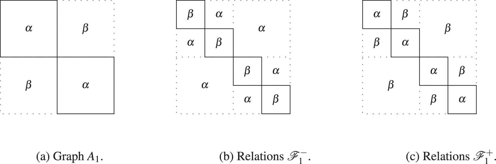
Benchmark model. Case 1.
In Table 2 we show the results obtained for different values of
5.2.2. Benchmark model. Case 2
It is known that the Louvain algorithm is very size sensitive. Nevertheless, in this subsection we show that our algorithm also works well when considering smaller communities. Here we define a standard structure in both relations graphs
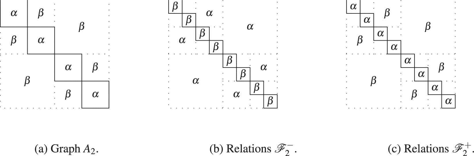
Benchmark model. Case 2.
5.2.3. Benchmark model. Case 3
The issue when working with previous benchmark models is that both may not fit well with reality, specially because all communities have the same size, and all nodes have the same expected degree. Then, an algorithm may work well in those benchmark graphs, but it is not as good at performing real-life examples. Hence, a good benchmark model should have a skewed degree distribution similar to real networks [42]. In general, algorithms should be tested on benchmarks of variable average degree and community size because these parameters may affect seriously the results. In an attempt to provide a better representation of reality, here we proposed a more complex structure: we consider asymmetric relations matrices
Benchmark model. Case 3.
5.2.4. Benchmark model. Case 4
Now we apply our algorithm in a very difficult model. Not only is the structure of the relations so asymmetric, but also the groups of the graph are somewhat small (see Figure 6). The adjacency matrix
Benchmark model. Case 4.
6. CONCLUSIONS
Given a set of elements between which there are some relationships, one of the most used mathematical tools for its representation are networks. The inconvenient of networks is that we cannot model all the information involved in a real-life problem with them. Here lies the importance of working with graphs which can include some additional information. This approach was first managed in [12], where it was proposed the idea of considering affinity relations among the nodes by means of extended fuzzy graphs. Nevertheless, not only positive evidences appear when modeling a real-life problem, but also negative evidence. In order to deal with this type of situation, in [7] it was introduced the idea of working with extended bipolar fuzzy graphs,
In a broader context, the key point of this paper is related to community detection problems based on multiple bipolar fuzzy measures. It is, in the resolution of clustering problems in which there exists some additional information about the relation among the nodes, which is defined by multiple bipolar fuzzy measures, and which is absolutely independent of the structure of the graph.
We start this paper with the definition of several concepts: the extended bipolar fuzzy graph and the bipolar weighted multi-graph associated with a bipolar fuzzy measure. Then, we generalize the notion of extended bipolar fuzzy graph, and the bipolar weighted multi-graph associated with a bipolar fuzzy measure, to the field of having multiple bipolar fuzzy measures. So, we introduce two notions: extended multiple bipolar fuzzy graph and the bipolar weighted multi-graph associated with multiple bipolar fuzzy measures. Then, focusing on OWA operators [34–37], we propose several “group” notions, based on multiple bipolar fuzzy relations. Both elements will be crucial for dealing with community detection problems in which there is some additional information about the relation between the nodes given by multiple bipolar fuzzy measures.
Apart of this, in Section 4 we provide a detailed explanation of the performance of Louvain algorithm. Then we propose a modification of this method, the
In order to quantify how each node of the graph is affected by the presence/absence of any other node in its clusters, depending on their relation in
Other important point of this article is the development of a wide analysis of the performance of our algorithm. To carry one with it, we provide some computational results with which we test the “goodness” of the Algorithm 3 (see Section 5 for more details). These tests consist in the generation of four different benchmark models [4,16,40], in combination with the calculation of the
Apart from this consideration of the contributions included in this paper, clearly devoted to community detection problems in graphs, let us emphasize the there are many more applications of this research. One of them is about the field of fuzzy relation equations. This type of fuzzy relation equations, are deeply analyzed in [43–45], comprises situations in which some unknown variables appear together with their logical negations, something closely connected with each pair of fuzzy measures
As further work, we propose different applications of Duo Louvain Algorithm, and, in particular, of the Multiple Bipolar Duo Louvain Algorithm, considering different operators
These two points are supposed to be our immediate further research. We would also like to extend our idea to FCMs [14]. FCM, usually used as decision support tools, are defined by nodes called concept and weighted edges called relationships. Then, an easy vision of FCM is considering them as directed and weighted networks whose edges defines cause and effect relations among the nodes, and the degree of these relations [13].
Moreover, we are working on the inclusion of additional information given by some fuzzy measure in the framework of different community detection algorithms, specifically, the method proposed by Girvan and Newman [30].
ACKNOWLEDGMENTS
This research has been partially supported by the Government of Spain, Grant Plan Nacional de I+D+i, MTM2015-70550-P, PGC2018096509-B-I00, and TIN2015-66471-P.
REFERENCES
Cite this article
TY  - JOUR
AU  - Inmaculada Gutiérrez
AU  - Daniel Gómez
AU  - Javier Castro
AU  - Rosa Espínola
PY  - 2020
DA  - 2020/10/22
TI  - Multiple Bipolar Fuzzy Measures: An Application to Community Detection Problems for Networks with Additional Information
JO  - International Journal of Computational Intelligence Systems
SP  - 1636
EP  - 1649
VL  - 13
IS  - 1
SN  - 1875-6883
UR  - https://doi.org/10.2991/ijcis.d.201012.001
DO  - 10.2991/ijcis.d.201012.001
ID  - Gutiérrez2020
ER  -