
Information Structures in an Ordered Information System Under Granular Computing View and Their Optimal Selection Based on Uncertainty Measures
- DOI
- 10.2991/ijcis.d.201007.001How to use a DOI?
- Keywords
- Ordered information system; Information granule; Information structure; Dependence; Information distance; Inclusion degree; Lattice; Map
- Abstract
Information structures (
- Copyright
- © 2020 The Authors. Published by Atlantis Press B.V.
- Open Access
- This is an open access article distributed under the CC BY-NC 4.0 license (http://creativecommons.org/licenses/by-nc/4.0/).
1. INTRODUCTION
Granular computing (GrC), presented by Zadeh [1,2], is a world view and methodology for viewing the objective world. Its main idea is to use granular thinking to solve complex problems, and transform them into the theory, method, technique and tool of the process of solving several relatively simple problems by abstracting and dividing complex problems.
An information granule (
An information system (IS) based on rough set theory was presented by Pawlak [7]. In GrC in an IS, the investigation of information structure (
Given an attribute of an IS, if the domain of this attribute is a partial order set in accordance with an increasing preference, then this attribute is a criterion in this IS. If every attribute of an IS is a criterion in this IS, then this IS is viewed as an ordered IS (an OIS). So far,
This article's research route is described in Figure 1.
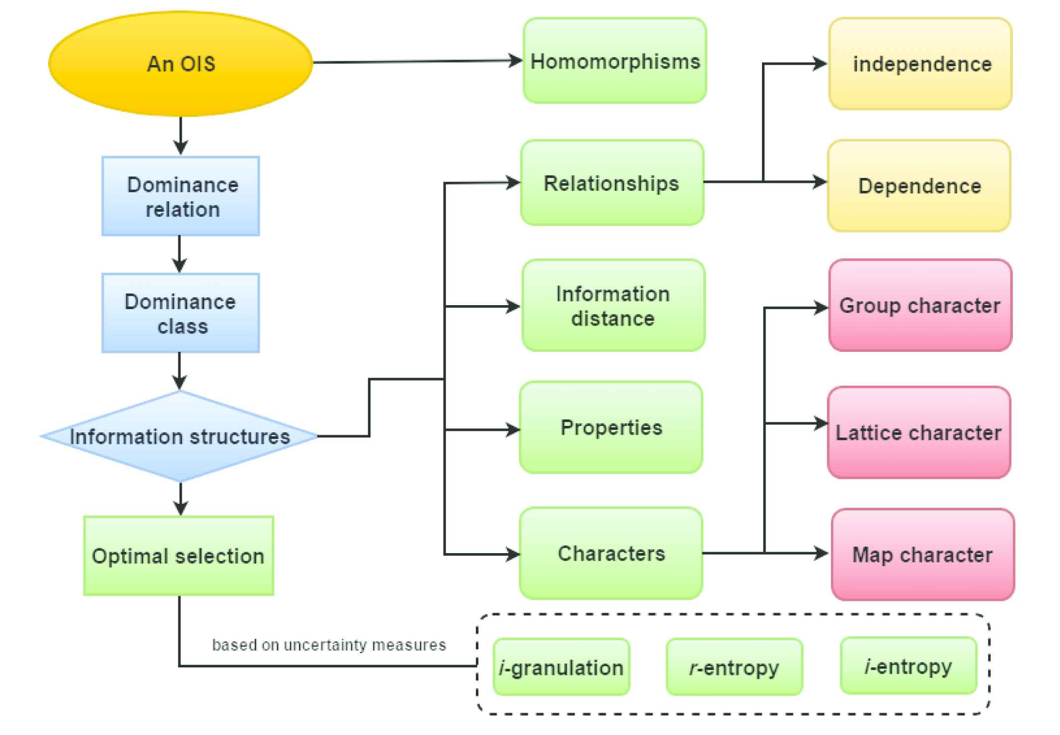
The work process of the article.
This article is organized as follows: Section 2 reviews some elementary concepts on binary relations, OISs and homomorphisms. Section 3 introduces
2. PRELIMINARIES
Throughout this article,
Put
2.1. Binary Relations
Throughout this article,
Suppose that
reflexive, if
symmetric, if
transitive, if
If
Given
2.2. An OIS
Definition 2.1. [7]
Suppose that
Definition 2.2. [18]
Let
In this article, an OIS is denoted by
Given
Given
Clearly,
Definition 2.3. [18]
Let
Then
Clearly,
Denote
Then,
Clearly,
Denote
Then
Proposition 2.4. [18]
Suppose that
Given
Given
Given
Let
It should be noted that
2.3. Homomorphisms between OISs
Communication between ISs is a significant subject in rough set, and could be viewed as a map between ISs. The notion of homomorphisms between ISs was first presented by Grzymala-Busse in [19,20].
Definition 2.5.
Assume that
The triple
Denote
3. THE CONCEPT OF i
Suppose that
Definition 3.1.
Assume that
If
Example 1.
Definition 3.2.
Let
Definition 3.3.
Let
Example 3.4. (Continued from Example 2.1 in [21])
Given an OIS
| 1 | 2 | 1 | |
| 3 | 2 | 2 | |
| 1 | 1 | 2 | |
| 2 | 1 | 3 | |
| 3 | 3 | 2 | |
| 3 | 2 | 3 |
An ordered information system (OIS)
Pick
Note that
Then
Then
4. RELATIONSHIPS BETWEEN i
4.1. Dependence and Independence between i
Definition 4.1.
Let
Example 4.2. (Continued from Example 3.5)
It can be obtained that
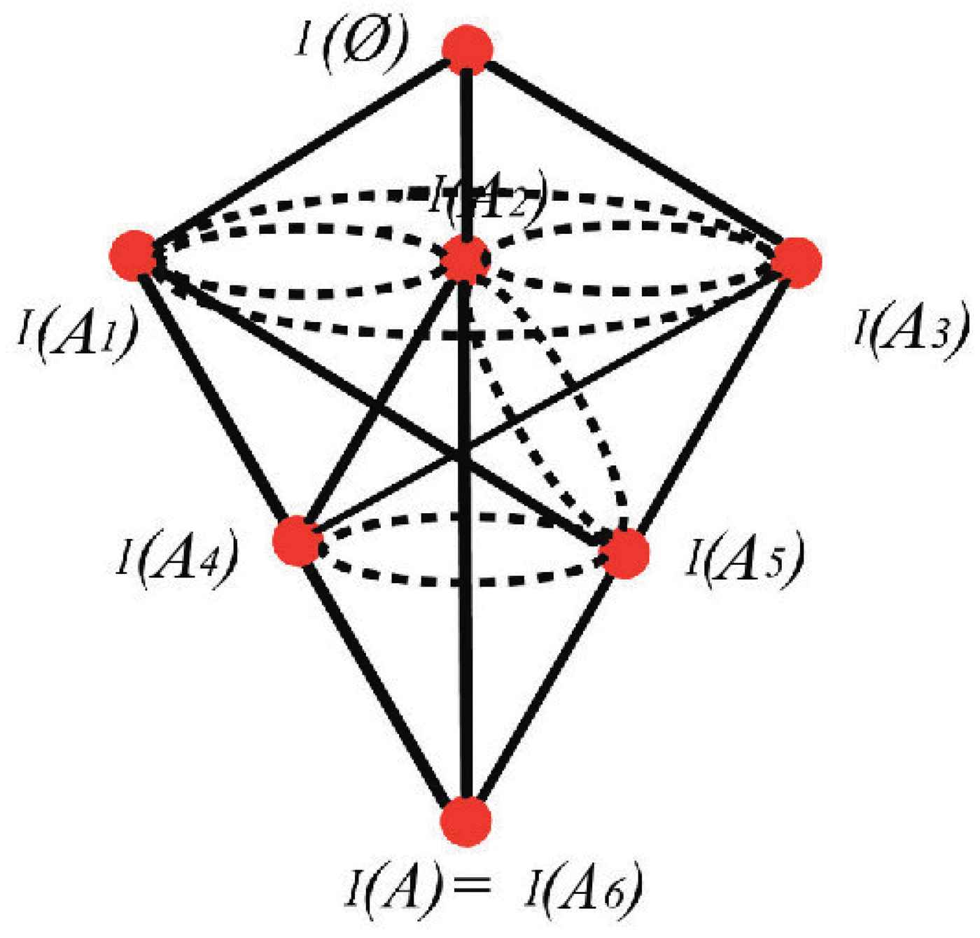
Relationships among
4.2. Information Distance between Two i
Definition 4.3.
Let
Theorem 4.7.
Let
Proof.
Assume
Clearly,
By Lemma 4.4,
By Lemma 4.5,
Then
So,
Proposition 4.8.
Let
If
If
Proof.
(1) Clearly,
Then,
Therefore
(2) Due to
Then,
Thus
(3) On account of
So,
Proposition 4.9.
Let
Proof.
It can be obtained that
Proposition 4.10.
Let
Proof.
Due to
By Lemma 4.6,
Example 4.11.
By Definition 4.3, one can obtain that
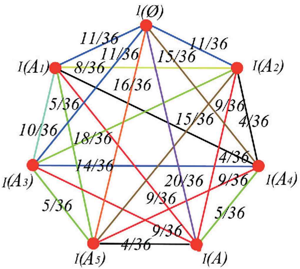 Figure 3
Information distance between
Let
It can be obtained that
On account of
On account of
5. PROPERTIES OF i
Theorem 5.1.
Let
Theorem 5.2.
Assuming
Proof.
Evidently.
Proposition 5.3.
Let
Proof.
On account of
Proposition 5.4.
Let
Proof.
It can be proved by Proposition 5.3.
Definition 5.5. [22]
Let
Definition 5.6.
Let
Proposition 5.7.
Proof.
Obviously.
Theorem 5.8.
Let
Proof.
Please see “Appendix.”
Corollary 5.9.
Let
Proof.
It can be proved by Theorems 4.7 and 5.8.
6. CHARACTERS OF i
In this section, we obtain group, lattice and map characters of
6.1. Group Characters of i
Theorem 6.1.
Proof.
Suppose
Clearly,
Thus
Additionally,
Thus,
Clearly,
Example 6.2.
By Theorem 6.1,
Additionally,
Then
Thus
6.2. Lattice Characters of i
Theorem 6.3.
Let
If
Proof.
Please see “Appendix.”
Corollary 6.4.
Example 6.5.
By Theorem 6.3,
It can be obtained that
Then
So
By Theorem 6.3,
Thus
Example 6.6.
It can be obtained that
Hence
6.3. Map Characters of i
Lemma 6.7.
Assume that
Proof.
“
On account of
So
Thus
“
Thus
Hence
Theorem 6.8.
Let
Proof.
By Lemma 6.7,
Then
Thus
Proposition 6.9.
Let
Proof.
Please see “Appendix.”
Corollary 6.10.
Assume that
Proof.
It can be proved by Proposition 6.9.
Theorem 6.11.
Assume that
Proof.
(1) It can be proved by Theorem 5.1 and Corollary 6.10.
(1) This follows from Theorem 5.2 and Proposition 6.9.
Corollary 6.12.
Let
Proof.
It can be proved by Theorem 6.11.
Theorem 6.13.
Assume that
Proof.
Please see “Appendix.”
Corollary 6.14.
Assume that
Example 6.15.
Assume that
| 2 | {0, 1} | 2 | 0.1 | {0} | 2 | 0.1 | 4 | 2 | 0.2 | |
| 6 | {0, 2} | 4 | 0.3 | {0, 1} | 4 | 0.2 | 4 | 4 | 0.2 | |
| 2 | {1} | 4 | 0.1 | {0, 1} | 4 | 0.2 | 2 | 4 | 0.1 | |
| 4 | {2} | 6 | 0.2 | {0, 1, 2} | 6 | 0.3 | 2 | 6 | 0.1 | |
| 6 | {0, 1, 2} | 4 | 0.3 | {1, 2} | 4 | 0.2 | 6 | 4 | 0.3 | |
| 2 | {0} | 4 | 0.1 | {0, 2} | 4 | 0.2 | 2 | 4 | 0.1 | |
| 2 | {0} | 4 | 0.1 | {0, 1} | 4 | 0.2 | 2 | 4 | 0.1 | |
| 6 | {1, 2} | 4 | 0.3 | {1, 2} | 4 | 0.2 | 4 | 4 | 0.2 | |
| 6 | {0, 1, 2} | 4 | 0.3 | {0, 1} | 4 | 0.2 | 6 | 4 | 0.3 | |
| 2 | {1, 2} | 2 | 0.1 | {1} | 2 | 0.1 | 4 | 2 | 0.2 | |
| 6 | {0, 2} | 4 | 0.3 | {0, 1} | 4 | 0.2 | 4 | 4 | 0.2 | |
| 6 | {0, 1, 2} | 4 | 0.3 | {1, 2} | 4 | 0.2 | 6 | 4 | 0.3 | |
| 6 | {0, 2} | 6 | 0.3 | {0, 1, 2} | 6 | 0.3 | 4 | 6 | 0.2 | |
| 2 | {2} | 4 | 0.1 | {0, 2} | 4 | 0.2 | 2 | 4 | 0.1 | |
| 6 | {0, 1} | 6 | 0.3 | {0, 1, 2} | 6 | 0.3 | 4 | 6 | 0.2 |
An ordered information system (OIS)
| 1 | 2 | 1 | |
| 3 | 2 | 2 | |
| 1 | 1 | 2 | |
| 2 | 1 | 3 | |
| 3 | 3 | 2 | |
| 3 | 2 | 3 |
An ordered information system (OIS)
A map
A map
Put
A map
Obviously,
Therefore
Pick
It is easy to verify that
Now, dependence and independence between
Pick
Note that
Clearly,
Then
Thus
From this example and these discussions, we can know that a complex massive OIS can be compressed into a relatively small-scale OIS and some same data structures can be received.
7. UNCERTAINTY MEASURES OF AN OIS AND THE OPTIMAL SELECTION OF i
In this section, we select the optimal
7.1. Uncertainty Measures of an OIS
Definition 7.1.
Consider that
In [21],
Theorem 7.2.
(Equivalence) Let
Proof.
It can be achieved by Definition 7.1.
Proposition 7.3.
Assume that
Moreover, if
Proof.
Since for each
By Definition 7.1,
If
If
Theorem 7.4.
Suppose that
If
If
Proof.
(1) This is obvious.
(2) By Definition 7.1,
Notice the
Consequently,
This theorem shows that when the available information turns into coarse, the
Proposition 7.5.
Assume that
Proof.
It can be proved by Theorem 7.4 and Proposition 5.3.
Definition 7.6. [21]
Suppose that
In [21],
Proposition 7.7.
Assume that
Furthermore, if
Proof.
Since
Then
By Definition 7.6,
If
If
Theorem 7.8.
Let
If
If
Proof.
(1) This is obvious.
(2) By Definition 7.6,
Note that
Hence,
Therefore
This theorem shows that the greater the uncertainty of the available information, the greater the
Proposition 7.9.
Given that
Proof.
This follows from Theorem 7.8.
Definition 7.10.
Let
In [21],
Theorem 7.11.
Let
Proof.
By,
But
Therefore
Example 7.12.
Proposition 7.13.
Assume that
Proof.
The proof is similar to Proposition 7.7.
Theorem 7.14.
Let
If
If
Proof.
(1) This is obvious.
(2) By Definition 7.10,
Note that
It is evident that
This theorem shows that if the structure of OIS turns into finer, the
Proposition 7.15.
Consider that
Proof.
It can be proved by Theorem 7.14.
7.2. Effectiveness Analysis
To evaluate the expression of the presented measures for the uncertainty of
Assume that
We select four datasets (i.e., Energy efficiency, Airfoil Self-Noise, QSAR fish toxicity and HCV for Egyptian patients) from UCI for effectiveness analysis.
Energy efficiency may express OIS
Airfoil Self-Noise may express OIS
QSAR fish toxicity may express OIS
HCV for Egyptian patients may express OIS
Then
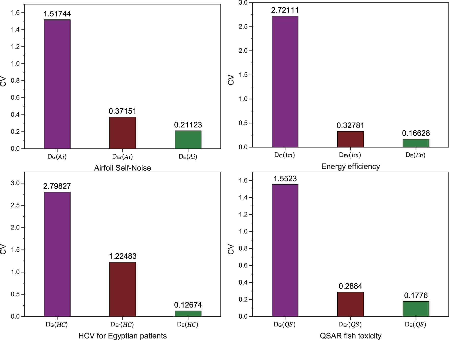
CV-values of three measure sets.
The dispersion degree of
Thus,
7.3. The Optimal Selection of i i
In this subsection, we select the optimize
Definition 7.16.
Let
If there exists
If there exists
The maximum
Theorem 7.17.
Let
Proof.
This follows from Proposition 7.5.
Example 7.18.
Pick
Then
Thus,
7.4. The Optimal Selection of i r
In this subsection, we select the optimal
Definition 7.19.
Let
If there exists
If there exists
The maximum
Example 7.20.
Pick
We have
Thus,
7.5. The Optimal Selection of i i
In this subsection, we select the optimal
Definition 7.21.
Let
If there exists
If there exists
The maximum
Example 7.22.
Pick
We have
Thus,
8. COMPARISONS
In this section, we make a comparison with literatures [11,23] so as to see the innovation of this article more clearly.
Three articles are based on GrC. Thus, the research ideas of three articles are the same and the obtained results are similar.
The research path of three articles is the same, and the details are as follows: Granular structures or
The differences of three articles are as below.
The studied ISs are different: This article considers
The introduced relations are different: This article introduces the dominance relation on the object set in an OIS by defining the order between two information values, literature [11] proposes the similarity relation on the universe in a covering IS by means of the neighborhood of each pointand literature [23] presents the tolerance relation on the object set in an incomplete interval-valued IS by defining the similarity degree between two information values.
The constructed
This article considers homomorphisms between OISs and then obtains map characters of
This article studies the optimal selection of
9. CONCLUSIONS
In this article,
Invariant characters of
CONFLICTS OF INTEREST
The authors declare that they have no conflict of interest.
AUTHORS' CONTRIBUTIONS
Y.N. Wang designs the overall structure of this paper and improves the language, S.C. Wang writes the paper, and H.X. Tang collects the data.
ACKNOWLEDGMENTS
The authors would like to thank the editors and the anonymous reviewers for their valuable comments and suggestions, which have helped immensely in improving the quality of the paper. This work was supported by Natural Science Foundation of Guangxi (2016GXNSFAA380282, 2018GXNSFAA294134), Guangxi Higher Education Institutions of China (Document No. [2019] 52), National Social Science Fund's Major Research Special Project (18VHQ013), China-ASEAN Institute for Innovation Governance and Intellectual Property Research (2019ZCY04), and Collaborative Innovation Center for Integration of Terrestrial and Marine Economies (2019YB22).
APPENDIX
Theorem 5.8.
Let
Proof.
(1) Obviously, “
“
Then
Then
Thus
It follows that
Hence
(2) “
Thus
“
Then
(3) It can be obtained from (2).
Theorem 6.3.
Let
If
Proof.
Clearly,
Assume that
Assume that
Hence
By the proof of Theorem 5.1, it can be obtained that
On account of
Assume that
Thus
Then
By Theorem 5.2,
Assume that
Hence,
Thus,
Clearly,
Proposition 6.9.
Let
Proof.
Suppose
Let
Then
Additionally,
So
Because
Then
This implies
Thus
Conversely, suppose
Because
Additionally,
Thus
On account of
Then
Because
Thus
Theorem 6.13.
Assume that
Proof.
Suppose
Let
Let
Additionally,
So
Because
This implies
On account of
Because
Then
So
This implies
Thus
Conversely, suppose
Let
Because
Additionally,
Then
On account of
Then,
So
Because
Thus
REFERENCES
Cite this article
TY  - JOUR
AU  - Yini Wang
AU  - Sichun Wang
AU  - Hongxiang Tang
PY  - 2020
DA  - 2020/10/21
TI  - Information Structures in an Ordered Information System Under Granular Computing View and Their Optimal Selection Based on Uncertainty Measures
JO  - International Journal of Computational Intelligence Systems
SP  - 1619
EP  - 1635
VL  - 13
IS  - 1
SN  - 1875-6883
UR  - https://doi.org/10.2991/ijcis.d.201007.001
DO  - 10.2991/ijcis.d.201007.001
ID  - Wang2020
ER  -