1. INTRODUCTION

The advancement in technology nowadays has enabled the collection and storage of datasets with massive number of features and large volume of data. An analyst may interest to analyze the features that distinguish a particular object from the rest of object in data set. In recent years, mining contrast subspace has been introduced to discover contrast subspaces of queried object. Given a two-class data set, a queried object, and a target class, mining contrast subspace finds subspaces where a queried object is most likely similar to target class while least likely similar to non-target class. Those subspaces are subsets of features that each can comprised of one or more features that represent the data set. These subspaces are called as contrast subspaces. Any object can be queried object which its contrast subspaces are unknown and need to be investigated. Target class is any class label on which the similarity to the queried object is examined in order to find contrast subspaces.

The discovery of contrast subspaces is a crucial task in many application domains including fraud detection, intrusion detection, medical diagnosis, etc. The contrast subspaces can be used to characterize a particular object and enhance the analysis of data. For instance, in banking sector, an analyst may want to know what subspaces do the suspicious transaction is most likely similar to fraudulent cases but dissimilar to normal cases. By knowing the contrast subspaces, further action can be taken in order to avoid the bank account being used by the unauthorized user. In addition to that, an analyst may want to identify the subspaces which cause a suspicious claim most similar to fraudulent cases but different from normal cases in an insurance sector [1,2]. Those contrast subspaces can help the analyst in determining the right action to be performed to tackle the misuse claim.

Tree-Based Contrast Subspace Miner (TB-CSMiner) is a tree-based mining contrast subspace method that finds contrast subspaces of a queried object in a two-class classification problem with continuous input variables [3]. It employs a tree-based likelihood contrast scoring function in estimating the likelihood contrast score of a queried object to the target class against the non-target class regardless of the number of features in the subspace. The tree-based likelihood contrast scoring function uses interval values of features to recursively partition a subspace space so that the queried object and the target samples are grouped together and separated from the non-target samples. It estimates the likelihood contrast score of subspaces with respect to the queried object based on the ratio of probability of target samples (e.g., objects belong to target class) to the probability of non-target samples (e.g., objects belong to non-target class). However, the tree-based likelihood contrast scoring function of TB-CSMiner is designed to estimate the likelihood contrast score of a subspace with respect to a queried object in a numerical dataset. Particularly, the partitioning criterion for the process of partitioning the dataset is formed based on the interval values of numerical feature. The partitioning process conducted based on interval values is not applicable for categorical dataset that takes unordered nominal values [4–7]. Thus, TB-CSMiner cannot be applied to handle categorical datasets directly. Mapping nominal values onto numerical or ordinal values may cause loss of information [5,6].

In real-life applications, many research works have been conducted to deal with categorical data in various data mining problem [4,5,8–14]. This indicates the importance of effectively mining contrast subspace to learn categorical datasets. Other works include summarizing relational datasets based on features selection which emphasized on discretization of numerical data into categorical data [15–17]. This paper addresses this issue by extending the TB-CSMiner method where a tree-based likelihood contrast scoring function is proposed for estimating the likelihood contrast score of subspaces with respect to queried object in a categorical dataset.

In a two-class categorical data set, given a subspace space and a queried object, the proposed tree-based likelihood contrast scoring function divides data objects into two subsets of objects repeatedly by using features values of queried object until the subset comprises of only objects belong to one class or the number of objects in the subset meets a minimum predefined threshold. Then, it measures the ratio of probability of target samples to the probability of non-target samples in the subset containing the queried object. Herein, the contrast subspace of a queried object is defined as the subspace where the queried object falls having higher probability number of target objects than the probability number of non-target objects. Since it is impractical to measure the likelihood contrast score of all possible subspaces, a similar framework of TB-CSMiner method is used to discover contrast subspaces of queried object in categorical dataset. That is, it first measures the likelihood contrast score of individual features or one-dimensional subspaces for the given queried object and selects only certain one-dimensional subspaces having high scores. This is followed by measuring the likelihood contrast score of possible subspaces for the queried object derived from the selected one-dimensional subspaces to find the contrast subspaces of queried object.

In this work, the effectiveness of the proposed extended TB-CSMiner method is validated in terms of performance accuracy of the classification task conducted on the resulting contrast subspaces. For a contrast subspace obtained from using the extended method, a new data set is generated by populating the contrast subspace space with the data sampled from the given data set in such a way that the target class and non-target class are separated well, with reference to a queried object. Subsequently, the newly created data set is used as an input for classification tasks. A contrast subspace shall achieve higher classification accuracy than other subspaces. The experimental results showed that the extended method has the ability to find contrast subspaces for the given queried object in categorical data.

The main contribution of this paper is to provide a tree-based method to find contrast subspaces of the target samples for categorical datasets. For a subspace, the tree-based method focuses on identifying a group of target samples having similar characteristics with the queried object. The tree-based method uses features values of queried object as criterion in partitioning the target and non-target samples. Based on the queried objects, the numbers of target and non-target samples are used to determine the similarity of queried object to the target class and non-target class in a subspace.

The remainder of this paper is organized as follows: Section 2 discusses related works. Section 3 presents the formalization of the tree-based likelihood contrast scoring function that deals with categorical values. The framework of the extended TB-CSMiner method which incorporates the proposed tree-based likelihood contrast scoring function for categorical data set is also presented in Section 3. Section 4 describes the experimental setup and results on eight real world categorical data sets. Finally, the paper is concluded in Section 5 by drawing a conclusion and providing some future works.

2. RELATED WORKS

There are a few methods have been developed to find contrast subspaces of a queried object to the best of our knowledge. Contrast Subspace Miner (CSMiner) is the earliest method introduced to discover contrast subspaces of the given queried object in numerical data set [1]. For a subspace, it employs the probability density of target class and the probability density of non-target class in the region where the queried object is located, to measure the respective likelihood score of the queried object to target class and to non-target class. The ratio of probability density of target class to probability density of non-target class is then used to estimate the likelihood contrast score of a subspace. A contrast subspace is where the queried object is in a region that comprised of higher density of target objects and lower density of non-target objects than average. This is corresponding to the queried object is most likely similar to target class and least likely similar to non-target class respectively. The likelihood contrast scores of contrast subspaces are often high compared to other subspaces. The CSMiner approach considers only non-trivial subspaces which their likelihood scores to the target class are not less than the predetermined minimum likelihood score in searching for contrast subspaces process. Besides that, CSMiner avoids the brute force search by using an upper bound of probability density of target objects to remove trivial subspaces from the search space. The possible subspaces are represented by an enumeration tree and the subspaces set are searched in depth-first search manner. All superspaces of a subspace (i.e., descendents of a subspace) can be removed if the upper bound of probability density of target objects does not meet the minimum likelihood threshold. CSMiner is remaining inefficient for data set with high number of features since the number of subspaces that need to be examined grows exponentially with the number of features in data set.

Contrast Subspace Miner-Bounding Pruning Refining (CSMiner-BPR) has been proposed to accelerate the process of CSMiner in searching contrast subspaces [2]. CSMiner-BPR combines a few new bounding pruning strategies and the pruning rule of CSMiner. CSMiner-BPR creates an upper bound of probability density of target objects and lower bound of probability density of non-target objects based on the ε-neighborhood of queried object. For each subspace, the neighborhood of a queried object is determined by the ε which is the marginal standard deviation of the data. Any objects within the distance ε of a queried object are assigned as the neighbors of the queried object. If the upper bound and lower bound conditions are met, all superspaces of a subspace can be pruned. By taking ε-neighborhood into account, it reduces the computation cost for objects outside from the ε-neighborhood and thus, speeds up the contrast subspaces search process.

However, CSMiner and CSMiner-BPR were developed for mining contrast subspaces in data set comprised of numerical values only. In both of these methods, the pair wise distance computation constituted their likelihood contrast scoring function. They used distance between objects to measure the similarity between objects. Unlike numerical values, categorical values are unordered and thus, it is difficult to define the similarity between categorical values by using distance [3,4]. This causes the existing methods cannot be directly applied to analyze categorical data set.

Recently, TB-CSMiner was introduced that applies a tree-based likelihood contrast scoring function to find contrast subspaces of the queried object in numerical data set [3]. The tree-based likelihood contrast scoring function adopts the divide-and-conquer concept of decision tree in measuring the likelihood contrast score of subspaces with respect to the given queried object. For a subspace, firstly, it selects a partitioning criterion to partition data objects including the queried object into two subsets of objects until the subset that containing the queried object reaches the predetermined minimum number of objects threshold or having objects belong to the same class. A partitioning criterion comprises a feature and its interval value which is the best for discriminating objects including queried object of different class. The likelihood contrast score of subspaces with respect to the queried object is then computed based on the ratio of probability of target objects to probability of non-target objects in the subset that containing the queried object. This also follows the notion applied in formulating the likelihood contrast score presented in the previous works (e.g., CSMiner and CSMiner-BPR) [1,2]. In contrast subspace, the queried object resides in subset that has higher probability of target objects and lower probability of non-target objects than the average value. That is, the contrast subspace should have high tree-based likelihood contrast score. TB-CSMiner accelerates the mining process by selecting a subset of one-dimensional subspaces with high likelihood contrast score from the initial features given in the data set. The contrast subspace of queried object is searched from those non-trivial one-dimensional subspaces. Although the tree-based likelihood contrast scoring function does not use distance in measuring the likelihood between the queried object and the class label, TB-CSMiner method cannot be applied directly for finding contrast subspaces of the queried object in categorical data. This is due to the categorical data contains features that take unordered nominal values. The partitioning criterion of the scoring function which is composed of the interval values of numeric feature cannot be used to partition categorical data in order to measure the likelihood contrast score of subspaces for a queried object.

Local Outlier with Graph Projection (LOGP) characterizes the abnormality of an object against the normal objects for categorical data by using the graph embedding approach [18]. It constructs geometrical structure model from the given data distribution and the model is used to find the subspaces where the object is well discriminated from the normal objects. In the problem of discovering properties, an algorithm called EXPREX was proposed that introduced the notion of exceptional property and defined the concept of exceptionality score, which measures the significance of a property [19]. Exceptional Property Extractor (EXPREX) identifies exceptional features with high exceptionality score for characterizing the abnormality of an object in categorical data. The exceptionality score is based on the randomization test following the Pearson chi-square criterion. A semi-supervised approach has been introduced for detecting outlier in categorical data [5]. It employs distance-based algorithm to characterize normal objects. This characterization model is used to identify outliers. Those features that contribute much in discriminating between normal objects and outliers are exploited in order to extract valuable information about the outlier. A feature-grouping-based outlier detection algorithm, WATCH method is proposed to identify outliers and explanation of the outlier in categorical data [20]. It gathered features into multiple groups based on the correlation among features. Then, it searched for outliers residing in each of the groups. The features group where the outliers are detected is used to explain the deviation of the outliers from other objects. Nevertheless, all of these methods find subspaces for explaining why an object is an outlier with respect to normal objects or inliers in categorical data. This is different from the proposed work in this paper in which the work focuses on finding subspaces where a queried object is most similar to target class than other classes in categorical data.

3. TB-CSMINER FOR CATEGORICAL DATA

In this section, an extended TB-CSMiner method is presented to discover contrast subspaces of the given a queried object in two-class categorical data. This method employs a tree-based likelihood contrast scoring function which is devised to estimate the likelihood contrast score of subspaces for a queried object in categorical data. In the next subsection, the formalization of new tree-based likelihood contrast scoring function utilized in the extended TB-CSMiner is presented. This is followed by a description of phases involved in the framework of the proposed extended TB-CSMiner to efficiently search for contrast subspaces in categorical data.

3.1. Tree-Based Likelihood Contrast Scoring Function

Given a two-class categorical data set, a queried object, and a target class, tree-based likelihood contrast scoring function uses features values of the queried object as partitioning criterion to group objects including queried object that have similar values on the features and also to separate the queried object from the non-target objects that have dissimilar values on the features in a subspace space. In fact, objects that have the same characteristics often belong to the same class and also belong to different class for objects that have dissimilar characteristics [21,22]. The tree-based likelihood contrast scoring function measures the likelihood score of a queried object to the target class and the non-target class based on the probability of target objects and the probability of non-target objects, in the group that contains queried object, respectively. Then, it uses the ratio of probability of target objects to probability of non-target objects to measure the likelihood contrast score of a subspace for the queried object.

The steps of the tree-based likelihood scoring measure process are described in the following. For a subspace space, it starts with choosing a criterion to partition data objects in the root node into a pair of nodes. Each of the nodes contains a subset of objects. We use the value of the selected feature of the given queried object as the partitioning criterion. For example, let consider the selected feature has value r for the given queried object, q, this value will be used for partitioning a node into a node containing subset of objects that have value r and another node which contains the rest of objects. A sequence of partitioning process is performed only on node where the given queried object falls. The partitioning process will be stopped when the number of objects in a node reaches a minimum number of objects threshold, MinObjs, or the nodes contains only objects belong to the same class. The node that has met one of the stopping criterions becomes the leaf node.

The likelihood contrast score of a subspace can be estimated based on the ratio of probability of target objects to probability of non-target objects in the leaf node. Sometimes, the leaf node can contain target objects without any non-target objects. In this situation, we use a small constant value n= 0.001 to replace the zero denominator of the probability of non-target objects which has been suggested in other relevant related works [23,24]. Let a queried object q and a dataset consists of objects O of two classes, O = O+∩O− where, O+ and O− are subsets of objects of O belong to target class C+ and non-target class C− respectively, described by a set of categorical features F, the tree-based likelihood contrast score of a subspace S for a q can be defined as following:

TB−LCS(q)=P(C+,Xleaf)∕|O+|n(1)

where P(C+,Xleaf) is the amount of target objects in the leaf node, |O+| is the amount of target objects in O,

n=P(C−,Xleaf)∕|O−|,P(C−,Xleaf)>00.001,P(C−,Xleaf)=0(2)

In Eq. (2), P(C−,Xleaf) is the amount of non-target objects in the leaf node and |O−| is the number of non-target objects in O. The value of P(C+,Xleaf) and P(C−,Xleaf) can be affected by the |O+| and |O−| respectively. Thus, |O+| and |O−| are used to normalize the respective P(C+,Xleaf) and P(C−,Xleaf). This corresponds to the probability of target objects and the probability of non-target objects in the leaf node. High tree-based likelihood contrast score of a subspace indicates that the queried object is more likely similar to the target class against the non-target class in the subspace. This means the subspace is likely to be the contrast subspace of the queried object.

Figure 1 depicts an illustration of TB−LCS(q) measure of three dimensional subspaces { s1, s2, s3} and { s2, s4, s6}. Suppose each feature in both of the subspaces has nominal values a, b, and c. The red point represents the queried object, the blue points signify objects that belong to target class, and the green points represent objects belong to non-target class. Let the minimum number of threshold MinObjs=5. For subspace { s1, s2, s3} in Figure 1, assume that the queried object has value b, a, and c for the respective feature s1, s2, s3, feature s1 having value b based on the queried object is selected first to partition the node that contains all objects in the data set into two groups, left node group and right node group. The left node group and right node group respectively comprise of objects that have feature s1 having values other than b and value b. Similar partition process continues using feature s2 having value a on the right node into which the queried object falls. After that, feature s3 having value c is selected to partition the right node. Since the queried object resides on the right node and there are only target objects in the node, the partition has been terminated at the third tier of the tree and the node becomes leaf node. The likelihood contrast score of subspaces { s1, s2, s3} is then computed.

Figure 1

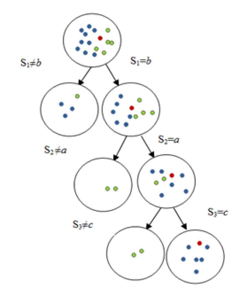
An illustration of TB − LC_S(q) computation subspace {s₁, s₂, s₃} for categorical data.

Meanwhile, for subspace { s2, s4, s6} in Figure 2, assume that the queried object has value b, a, b for each feature in the subspace respectively. The partition process begins by selecting feature s4 having value a following the s4 of the queried object and proceeded on the right node group that contains the queried object using feature s6 having value b. Lastly, the feature s2 habing value a is then used to partition the right node where the queried object falls. The partition process is halted on the right node at the third tier of the tree as the amount of objects in the node is less than MinObjs. That node becomes leaf node and subsequently the likelihood contrast score is calculated for subspace { s2, s4, s6}.

Figure 2

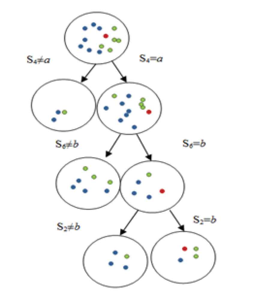
An illustration of TB − LC_S(q) computation subspace {s₂, s₄, s₆} for categorical data.

Based on the likelihood contrast score estimation for subspace { s1, s2, s3} and { s2, s4, s6}, the subspace { s1, s2, s3} is identified as the contrast subspace of the given queried object. This is undeniable as there are target objects only in the leaf node which corresponds to the queried object is more likely similar to the target class against non-target class.

3.1.1. The framework of extended TB-CSMiner method

When the number of features in categorical data set is high, the number of subspaces derived can be huge. This causes inefficient to compute the TB−LCS(q) of each subspace for a queried object. Feature selection is well known with its ability to accelerate the process of mining through reducing the dimensionality of data and at the same time it can improve the mining accuracy by eliminating the trivial features [25–28]. Hence, similar to the TB-CSMiner, the extended method comprises two main phases that are the feature selection and the contrast subspace search. The framework of two phases extended TB-CSMiner method is illustrated in Figure 3.

Figure 3

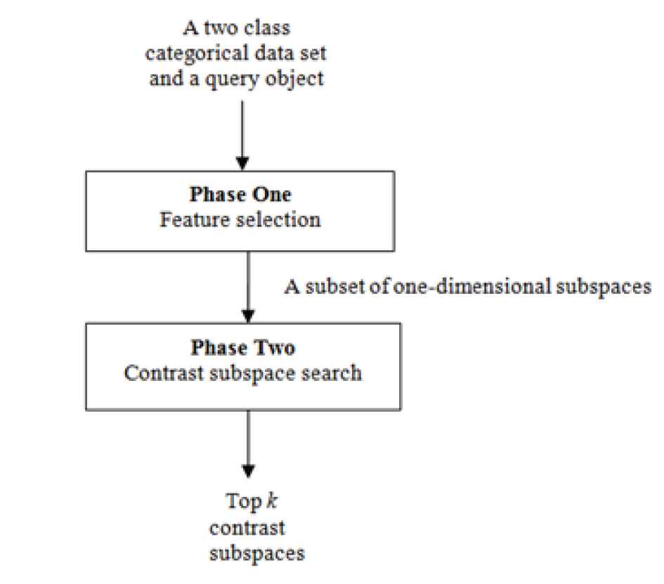
Framework of extended Tree-Based Contrast Subspace Miner (TB-CSMiner) method.

The pseudo code for phase one is presented in Algorithm 1 as shown in Table 1. In phase one, the tree-based likelihood contrast score of a subspace S for a given queried object q of a one-dimensional subspace in the categorical data set, is computed by using the devised TB−LCS(q) scoring function specifically for categorical data as shown in Eq. (1). The subspace is then compared with the subspaces in the current list of l one-dimensional subspaces by their likelihood contrast scores. If there is a subspace in the list which its likelihood contrast score is lower than the score of the currently considered subspace, the subspace in the list is removed and replaced with the considered subspace. After finished assessing each of the one-dimensional subspaces given in the data set, the subspaces are sorted in descending order of their TB−LCS(q) scores. These top l ranked one-dimensional subspaces are selected as a subset of non-trivial subspaces for contrast subspaces search in phase two. The parameter l is a predetermined number of one-dimensional subspaces.

Algorithm 1 Feature selection

Input: queried object q, target class C+, categorical data set X, set of categorical features F, minimum number of objects MinObjs, number of one-dimensional subspaces l Output: Subset of l one-dimensional subspaces with highest tree-based likelihood contrast score 1 Initialize Fs as list of l null subspaces with tree-based likelihood contrast score 0 2 For one-dimensional subspace s∈F 3    If ∀o∈X belong to same class or |X|⩽ MinObjs 4      Compute TB−LCs(q) using Eq. (1); 5      S ← s; 5      If ∃ S' ∈ Fs s.t. TB-LCS(q) > TB-LCS‘(q) 6        Insert S into Fs and remove S' from Fs; 7      End 8    Else 9      Select the s value of q to partition X; 10     X ← subset of data containing q after partition; 11   End 12   Sort Ans in descending order of TB-LCs(q); 13 End for 14 Sort Fs in descending order of TB-LCs(q); 15 Return Fs;

Table 1

Pseudo code for feature selection phase.

Algorithm 2 provides the contrast subspace search procedure in phase two depicted in Table 2. In phase two, the TB−LCS(q) score of t random subspaces with respect to the queried object are assessed to find contrast subspaces of the queried object. First, a feature is randomly picked from the subset of selected one-dimensional subspaces. Herein, the value of the feature based on the given queried object is then used as a partitioning criterion to partition data space with respect to the queried object. These processes are performed repeatedly until the stopping criterions as mentioned in the previous section are met. The different features along the partition are taken as a random subspace. After that, the devised TB−LCS(q) function specifically for categorical data in Eq. (1), is used to compute the TB−LCS(q) score of the subspace. Then, the TB−LCS(q) score of the subspace is compared with the score of subspaces in the current list of k subspaces. The subspaces in the list with TB−LCS(q) score lower than the score of the current subspace being considered are removed from the list and then, the considered subspace is appended to the list. When t random subspaces have been constructed and examined, the k subspaces in the list are ordered by their TB−LCS(q) scores from the largest score to the smallest score. Finally, the h highly scored subspaces are selected as the contrast subspaces of the queried object.

Algorithm 2 Contrast subspace search

Input: queried object q, target class C+, categorical data set X, set of one-dimensional subspace Fs, minimum number of objects MinObjs, number of contrast subspaces h, number of random subspaces t Output: h contrast subspaces with highest tree-based likelihood contrast score 1 Initialize Ans as list of h null subspaces with tree-based likelihood contrast score 0 2 For i:=1:t do 3    S ←∅; 4    Select a random feature s from Fs; 5    Select the s value of q to partition X; 6    X ← subset of data containing q after partition; 7    If ∄ s′∈ S s.t. s′ = s 8      Insert s into S; 9    End 10  If ∀o∈X belong to same class or |X|⩽ MinObjs 11      Compute TB−LCs(q) using Eq. (1); 12      If ∃ S' ∈ Ans s.t. TB-LCS(q) > TB-LCS‘(q) 13        Insert S into Ans and remove S' from Ans; 14      End 15    Else 16      Go to Step 4; 17    End 18    Sort Ans in descending order of TB-LCs(q); 19 End for 20 Return Ans;

Table 2

Pseudo code for contrast subspace search phase.

4. EXPERIMENTAL SETUP

5. RESULTS AND DISCUSSION

The results of all classifiers on eight real-world categorical data sets for full-dimensional subspace and contrast subspace are reported in Table 4.

Refering to Table 4, the average classification accuracies of the classification tasks performed by the J48 classifier using the contrast subspace space dataset were higher compared to the one using the full-dimensional space for all data sets except Mushroom data. That is, the J48 classifier achieved 84.56%, 88.23%, 98.58%, 94.99%, 90.78%, 97.69%, 95.04%, and 89.82% for the respective Mushroom, Breast Cancer, Congressional Votes, Tic-Tac-Toe, Lymphography, Chess, Car Evaluation, and Heart data. While for the NB classifier, it shows high average classification accuracy for the contrast subspace compared to the average classification accuracy for the full-dimensional subspace of the Breast Cancer, Congressional Votes, Tic-Tac-Toe, Lymphography, Chess, and Heart datasets. The NB classifier achieved 86.27%, 89.83%, 98.32%, 95.71%, 91.85%, 98.03%, 95.53%, and 91.52% for Mushroom, Breast Cancer, Congressional Votes, Tic-Tac-Toe, Lymphography, Chess, Car Evaluation, and Heart datasets, respectively.

Similarly, the Random Forest (RF) classifier gained high average classification accuracy on contrast subspace compared to the average classification accuracy on full dimensional subspace for Breast Cancer, Congressional Votes, Tic-Tac-Toe, Lymphography, Chess, and Heart data. Particularly, RF achieved 86.74%, 89.85%, 98.84%, 95.37%, 91.69%, 98.22%, 95.45%, and 90.97% for the respective Mushroom, Breast Cancer, Congressional Votes, Tic-Tac-Toe, Lymphography, Chess, Car Evaluation, and Heart data. On the other hand, the average classification accuracy of the classifier SVM on contrast subspace is higher than the average classification accuracy of the classifier SVM on full-dimensional subspace for five data sets which are the Breast Cancer, the Congressional Votes, the Tic-Tac-Toe, the Lymphography, and the Heart data. It achieved 86.14%, 86.88%, 98.45%, 95.25%, 86.31%, 97.65%, 95.37%, and 89.64% for the respective Mushroom, Breast Cancer, Congressional Votes, Tic-Tac-Toe, Lymphography, Chess, Car Evaluation, and Heart data. However, the performance accuracy of the classifiers was lower when using the contrast subspace of the Mushroom and Car Evaluation datasets. This happened because of the high number of objects in Mushroom and Car Evaluation data may require high minimum number of objects in the leaf node to estimate the similarity between the queried object and the target samples. Meanwhile, the classifiers performed very well for the contrast subspace than full dimensional subspace of the Breast Cancer, Congressional Votes, Tic-Tac-Toe, Lymphography, and Heart datasets. This may be due to the fact that those data comprised of only small number of objects. Although there are advanced approaches able to achieve high performance accuracy on some of the data sets, those approaches attempt at either classifying object to a class or searching clusters of objects that are having similar characteristics [38,39]. However, our work interest is to find contrast subspaces for a particular queried object where queried object is most similar to target class against other class.

The classification accuracies obtained using the NB and RF classifiers for the contrast subspace space often provide high classification accuracy compared to other classifiers. This is due to the classifier NB involves probability estimation in classifying data which is similar to the tree-based likelihood contrast scoring function of the tree-based method that estimates the probability of target objects and other objects with respect to the queried object in finding contrast subspaces. Meanwhile, the RF classifier creates multiple random decision trees, thus it reduces the over fitting issues and hence improves the classification accuracy. The SVM classifier produced low classification accuracy for the contrast subspace space compared to the other classifiers on most of the datasets. This is because proper approaches are necessary for SVM to deal with data consisting more than two classes [35].

Overall, the classification tasks being carried on contrast subspace space outperform most of the classification tasks on full-dimensional space that is 24 out of 32 various cases. The classification tasks on full-dimensional subspace outperform the classification tasks on contrast subspace on only eight out of 32 various cases. The superior performance on contrast subspace indicates that the contrast subspaces obtained by using the extended tree-based method is capable to improve the accuracy of the classification tasks. This is due to the fact that the objects of two classes are separated well in contrast subspace space. According to the paired-sample T-test at the significance level of 0.05, the extended tree-based method has achieved significant improvement of classification accuracy against the baseline classification (i.e., classification on full-dimensional space) on most of cases. In summary, the results demonstrate that the extended method exhibits the ability to identify the right contrast subspaces for the given queried objects in categorical data set.

6. CONCLUSION

There are many data contains categorical values in real-life applications. It often requires methods specifically designed for handling those categorical data in order to attain satisfactory performance. In this paper, we have extended the TB-CSMiner for finding contrast subspaces of a given queried object in two-class categorical data set. It uses a tree-based likelihood contrast scoring function that has been designed to handle nominal values of categorical data. The extended method comprises of two phases; Phase (1) finding a subset of relevant one-dimensional subspaces from initial features given in dataset and Phase (2) performing contrast subspace search on the selected subset of one-dimensional subspaces, with respect to a given queried object. We have experimentally evaluated the effectiveness of our extended method on eight real-world categorical data sets. These empirical studies have shown that the extended method was capable to improve the classification accuracy and mine contrast subspaces of a given queried object in categorical data. One of the future works of this paper will be improving the efficiency of mining process and optimizing the contrast subspace search using an evolutionary algorithm.

AUTHORS' CONTRIBUTIONS

This is to inform the editor that all Authors have contributed equally to the publication of this paper.

ACKNOWLEDGMENTS

This work was supported in part by the Universiti Malaysia Sabah internal grant no. SBK0428-2018.