
Feature-Weighting and Clustering Random Forest
 , Tao Wen1, 2, Wei Sun2, Qilong Zhang1
- DOI
- 10.2991/ijcis.d.201202.001How to use a DOI?
- Keywords
- Random forest; Feature weighting; Node split method; Categorical feature; Decision tree ensemble
- Abstract
Classical random forest (RF) is suitable for the classification and regression tasks of high-dimensional data. However, the performance of RF may be not satisfied in case of few features, because univariate split method cannot bring more diverse individuals. In this paper, a novel method of node split of the decision trees is proposed, which adopts feature-weighting and clustering. This method can combine multiple numerical features, multiple categorical features or multiple mixed features. Based on the framework of RF, we use this split method to construct decision trees. The ensemble of the decision trees is called Feature-Weighting and Clustering Random Forest (FWCRF). The experiments show that FWCRF can get the better ensemble accuracy compared with the classical RF based on univariate decision tree on low-dimensional data, because FWCRF has better individual accuracy and lower similarity between individuals. Meanwhile, the empirical performance of FWCRF is not inferior to the classical RF and AdaBoost on high-dimensional data. Furthermore, compared with other multivariate RFs, the advantage of FWCRF is that it can directly deal with the categorical features, instead of the conversion from the categorical features to the numerical features.
- Copyright
- © 2021 The Authors. Published by Atlantis Press B.V.
- Open Access
- This is an open access article distributed under the CC BY-NC 4.0 license (http://creativecommons.org/licenses/by-nc/4.0/).
1. INTRODUCTION
The performance of classifiers can be significantly improved by aggregating the decisions of several classifiers instead of using only a single classifier. This is generally known as ensemble of classifiers, or multiple classifier systems. For an ensemble to achieve better accuracy than individual classifier, it is critical that there should be sufficient independence or dissimilarity between the individual classifiers.
The decision trees (DTs) are unstable classifiers, because when the training set is changed slightly, the prediction results may change greatly [1]. Therefore, DTs become the ideal candidates as the base classifiers in various ensemble learning frameworks. Random forest (RF) is a paragon of such ensembles, and is suitable for the classification and regression tasks of high-dimensional data and ill-posed data. RF is widely used in gene expression [2], credit risk prediction [3] and other fields [4] because of its excellent generalization ability, fast training speed, parallel processing, robustness to noise, few parameters, embedded feature selection.
RF is proposed by Breiman in [5]. In that paper, bootstrap sampling was used on training set to obtain a large number of random sampling subsets, and a DT was constructed based on each sampling subset. To further reduce the similarity between trees in the forest and speed up the construction of the trees, a subset of the features is selected randomly when each node in a tree is split, and the suitable split hyperplanes could be searched in the subspaces of features. In the prediction, the tree votes are combined by majority voting.
In contrast to the Adaboost [6], RF has obvious advantages in the construction speed and the robustness, which are attributed to the adoption of “random subspaces” strategy in node splits. As Ho said in [7]: “While most other classification methods suffer from the curse of dimensionality, this method can take advantage of high dimensionality.” RF is very suitable for the classification and regression tasks of the high-dimensional and sparse data. However, for low-dimensional data, the DTs in RF have higher similarity which leads to the poor generalization ability of ensemble classifier. To improve this situation, the oblique DTs are considered as base classifiers. Murthy et al. [8] shows that there are
In Breiman [5] posed a simple random oblique split method. But according to the experimental results, we can see that there was no advantage compared with the axis-parallel split. With the emergence of oblique DT algorithms, some oblique split methods with low computational consumption are used in ensembles [9–11]. These ensembles inherit the characteristics of RF, such as high efficiency, adapting to high-dimensional data, and have exceeded the performance of classic RF in some application fields. However, the oblique split methods are only adapted to the numerical data. When handling the data containing discrete and disordered categorical features, these ensembles need to convert the categorical features to numerical features by CRIMCOORD [12], OneHot encoder or other methods. The conversion may bring new bias to the classification tasks and reduce the generalization ability of classifiers. In Bjoern et al. [10], it has been shown that the performance of these methods on categorical data is not as good as that of classical RF.
In this paper, we present a method of node splits based on feature-weighting and clustering, which can not only combine multiple numerical features, but also combine multiple categorical features without conversion. And this split method working with the strategy of “random subspace” can construct more diverse DTs for ensemble. Therefore, based on the framework of RF, we use this split method to construct DTs. The ensemble of the DTs is called FWCRF. The experiments show that FWCRF has excellent generalization ability on numerical data, categorical data and mixed data. Especially, on the low-dimensional data, the performance of FWCRF outperforms classical RF.
The rest of the paper is as follows: Section 2 is the related work about brief reviews. The details of our split method and ensemble method will be given in Section 3. In Section 4, we compare the FWCRF with AdaBoost and RF through experiments. Section 5 gives our conclusion.
2. RELATED WORKS
In this section, we will briefly review node splits in DTs and ensembles of DTs first.
2.1. Split Methods
In Ho [7], on the premise of only considering the numerical data, the author divided the linear splits of nodes into three classes: axis-parallel linear splits, oblique linear splits and piecewise linear splits. The axis-parallel methods only act on one dimension at a time and thus result in an axis-parallel split. Besides, a suitable cut point (
The famous C4.5 [13] and CART [14] are axis-parallel trees, which have the advantages of fast induction and interpretability. However, if candidate features are strongly correlated, an extremely bad situation may occur. In Figure 1, it is easy to see that the features A1 are strongly related to each other. To completely separate the two classes of samples, multiple axis-parallel splits are needed which will result in a complex DT structure. So, the axis-parallel splits reduce the interpretability of the model and lead to over-fitting due to sufficiently detailed splits, thus influencing the generalization ability.
Axis-parallel splits and oblique split.
The oblique split methods can deal with the problem shown in Figure 1. In the space of p-dimensional numerical features, the samples in the node are divided into the left node or right node according to (2).
In (2), al is the coefficient of the lth feature, and if the
Different from binary-way splits of axis-parallel and oblique methods, piecewise linear method is multi-way splits. As Figure 2 illustrated, piecewise linear splits are regarded as the combination of multiple oblique splits. The methods can be simply described as: looking for k anchors in feature space, and each sample is clustered according to the nearest neighbor anchor. The anchors here may be selected among training samples, class centroids or cluster centers. Pedrycz and Sosnowski [19], Li et al. [20] and our method fall into this class.
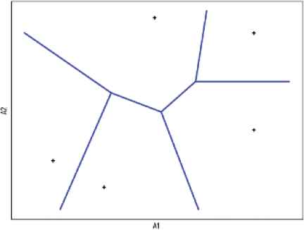
Piecewise linear splits.
2.2. DT Ensembles
Boosting [6], Bagging [21], Random Subspaces [7] and RF [5] are classic in ensemble learning.
AdaBoost is the most famous representative of Boosting. In Boosting, the individual classifiers are added one at a time so that each subsequent classifier is trained on data which have been “hard” for the previous ensemble members. A set of weights is maintained across the samples in the data set so that samples that have been difficult to classify acquire more weight, forcing subsequent classifiers to focus on them. The weights are also used in final decision combination, and the weights are determined by accuracies of individual classifiers.
In Bagging, the training subsets for generating the individual classifiers are extracted from the original training set based on bootstrap method, and the majority voting method is used for decision of ensembles. Bagging is suitable for parallel implementation for fast learning. However, the diversity obtained by bootstrapping is not as good as Boosting.
Different from the Boosting and Bagging based on random subsampling, the random subspace method selects feature subsets randomly to construct individual classifiers. The experiments in [7] show that random subspace method can produce more diverse individuals than Boosting and Bagging.
RF is an extension of Bagging, which combines random subsampling and random subspace. RF not only inherits the parallelizable characteristic of Bagging, but also has fewer randomly selected features in the process of constructing the individual trees, which makes RF achieve the accuracy compared favorably with AdaBoost, and the construction speed is much faster than the latter.
The effectiveness of RF does not depend on the specific methods of DT induction, and the oblique splits and piecewise linear splits can also be used to construct trees in forest, such as principal components analysis (PCA) [9,22], linear discriminant analysis (LDA) [10], support vector machine (SVM) [11] and C-fuzzy clustering [23]. In some cases, these methods can bring about better individual “accuracy” and “diversity.” However, PCA, LDA and SVM cannot be directly applied to categorical data.
3. FWCRF
The generalization ability of ensemble depends not only on the accuracy of individual DTs, but also on individual diversity. When the samples and features are sufficient, the univariate DTs with fast construction speed are more suitable to be the base classifiers of the ensembles. Instead, if the samples or features are insufficient, the multivariate split methods will bring about more diverse individuals for the ensembles. However, most multivariate split methods can only be used for numerical data. The feature-weighting and clustering split method proposed in this paper is based on the combination of multiple variables, and it is suitable to deal with the data of numerical features, categorical features and mixed features. The DTs constructed by this method have better generalization ability than the univariate DTs. The split method proposed can bring more diverse individuals to the ensembles by combining the “subsampling” and “subspace,” so that it ensures the better generalization ability of the ensembles compared with the classical RF in case of fewer training samples or features.
3.1. Feature-Weighting and Clustering Split
The split method proposed is based on clustering assumption. The clustering assumption states that the samples belonging to the same cluster belong to the same class. K-means is a widely used clustering algorithm. In this paper, we adopt the improved K-means to split nodes.
The number of classes of the current node is regarded as the clustering number k. The n samples in training set D will be divided into k disjoint subsets,
In (3),
Repeat (3) and (4) until the preset number of iterations is reached or the positions of all cluster centers are no longer changed.
The original K-means is an unsupervised clustering algorithm, which is suitable for unlabeled data. And the optimization goal is to minimize (5).
The goal of split is to reduce the class impurity of current node as much as possible. Note that the two goals are not the same. Therefore, we estimate the correlations between features and label to weight features. When calculating the distance from a sample to a cluster center, we give a larger weight to the feature strongly related to the label that enlarges the contribution of the feature to the distance. Otherwise, we give a smaller weight that reduces the contribution of the uncorrelated feature to the distance. In this way, the optimization goal of K-means algorithm is close to that of node split.
In this paper, we use the Relief-F algorithm [24,25] to weight features. The algorithm picks m samples. For each sample R, its knn nearest neighbors are searched in each class. The weight of feature A is calculated as follows:
In order to illustrate the role of feature weighting in clustering, we use dataset iris to carry out a simple experiment: 150 samples of dataset iris come from three classes, and each class has 50 samples. We directly use K-means algorithm to cluster, and obtain 10 misclassified samples. The specific results are shown in the confusion matrix in Table 1.
| setosa | versicolor | virginica | |
|---|---|---|---|
| Child node 1 | 50 | 0 | 0 |
| Child node 2 | 0 | 44 | 4 |
| Child node 3 | 0 | 6 | 46 |
Split results of unweighted features for iris.
Then, we use the Relief-F algorithm to calculate the weights of four features, which are 0.09, 0.14, 0.34 and 0.39 respectively. In the process of K-means clustering, the distances between samples and cluster centers are calculated by (8), where p indicates the number of features, wl indicates the weight of the lth feature. We obtain 6 misclassified samples, and the specific results are shown in Table 2.
| setosa | versicolor | virginica | |
|---|---|---|---|
| Child node 1 | 50 | 0 | 0 |
| Child node 2 | 0 | 48 | 4 |
| Child node 3 | 0 | 2 | 46 |
Split results of weighted features for iris.
Our method can be simply described as feature-weighting and clustering two steps. The specific process is shown in Algorithm 1.
In Algorithm 1, Imax value in the range of 1–10 with the probability of uniform distribution.
In step 3 of Algorithm 1, Relief-F is used to get the weights. Time complexity of Relief-F is
Steps 7 to 12 are the clustering process, and the time complexity is
Algorithm 1: split
Input: Current node training dataset D
Output: Divide D as
1: Initilize the number of clusters k with the number of classes in D.
2: Select feature subset F, randomly.
3: Input D and F, call Relief-F to generate w.
4: Assign wmax with maximum in w, F excludes features whose weights are less than
5: Initialize
6: For 1 to Imax Do
7: Combining (3) and (8), divide samples into
8: Recalculate
9: If
Then break For
10: End For
11: Return
Considering the above two parts, the time complexity of the Algorithm 1 is
OC1 [8] is a classic oblique DT, whose time complexity is
In summary, when k is small, the efficiency of the proposed split method is close to classical axis-parallel split method, and is better than most oblique split methods.
3.2. Categorical Feature
As mentioned in the previous subsection, the split method can be directly applied to numerical features. For categorical features, Relief-F algorithm can still be used to weight features. However, in the process of clustering, the representation of cluster center and the distance from sample to cluster center need to be redefined.
Inspired by the algorithms K-modes [26] and K-summary [27], in this paper, we use the probability estimation of each categorical feature value to represent the cluster center, and define a function to calculate the distance from sample to cluster center.
Definition 1.
Sj,l is the summary of all values of Al in Cj, and defined as follows:
Definition 2.
The center of Cj is represented by the following vector:
Definition 3.
Definition 4.
Let's use an example to illustrate the above definition. Suppose there are two clusters C1 and C2 described by two categorical features A1 and A2, and each cluster contains 10 samples as is shown in Table 3.
| A1 | A2 | |
|---|---|---|
| C1 | a11:9, a12:1 | a21:4, a22:4, a23:2 |
| C2 | a11:4, a12:3, a13:3 | a21:4, a22:4, a24:2 |
The distribution of values.
According to (10) and (11), the centers of C1 and C2 are
Only considering the categorical feature data, in Algorithm 1, we use (11) to represent clustering center instead of the original ones in step 5 and 8, and use (13) to calculate the distance from sample to cluster center instead of (8) in step 7.
For mixed feature data, the vector of clustering center consists of two parts: one is the means of numerical features, and the other is the vector as shown in (11). In this case, we use (14) to calculate the distance from sample to cluster center, where dis_n and dis_c are obtained by (8) and (13) respectively. And
3.3. The Constructions of DTs
In FWCRF, the trees are constructed on the basis of the top-down and recursion, and the split should be stopped, only when all samples in the current node are the same class or the feature subset used cannot distinguish these samples. The specific process is shown in Algorithm 2.
Algorithm 2: create_tree
Input: training set Ds
Output: the decision tree
1: Create node according to the samples in Ds.
2: Procedure grow(node)
3: If All the samples are of the same class or have the same feature values Then
4: Mark the node as a leaf, and label it with the class of the majority of samples in Ds.
5: Return node
6: End If
7: Call split to get the cluster
8: Save the values of
9: For
10: Create node_i according to samples in Ci, call grow(node_i).
11: End For
12: End Procedure
13: Return the node-rooted decision tree.
3.4. The Forest Construction and Combination Prediction
RF and Bagging use bootstrap method to independently and randomly select the subsets of the raw training samples with replacement. In this way, some samples will appear repeatedly in the same sample subset. However, we don't follow the method when we build the forests. The reason is that we use the Relief-F algorithm to weight the features in the split processing. The duplicate samples will affect the selection of the neighbors and cause feature weight to be enlarged. FWCRF extracts ns samples from the original training set D to form a subset Ds, using a randomly stratified sampling method without replacement. The ns is a parameter determined by users. The Ds is used to train an individual classifier. The data that are not sampled consists of out-of-bag dataset Do,
In (15), the acc and err represent the number of correctly classified samples and misclassified samples of Do on the leaf node, respectively.
nt and nf are the parameters in FWCRF, and nt represents the size of forest and nf determines the dimension of random subspace F in Algorithm 1. Users can adjust these parameters to trade off the accuracy and diversity of individual classifiers to achieve satisfactory ensemble accuracy and execution speed. The reason why these parameters should be decided by the users is that the way that can be applied to all classification problems is not available at present. The forest construction process is shown in Algorithm 3.
Algorithm 3: create_forest
Input: training set D, ns, nt and nf
Output: the forest
1: Create an empty forest Fo.
2: For
3: Sample randomly to obtain Ds and Do via D.
4: Use Ds to generate Ti.
5: Use Do to calculate the voting confidence of each leaf node in Ti.
6: Add Ti to Fo.
7: End For
8: Return Fo
The combination prediction is realized by (16).
In (16), Fo(x) and Ti(x) represent the decisions of the forest and the ith tree on the sample x, and
4. EXPERIMENT
In this section, we implement experiments to compare the performance of FWCRF with classic RF and AdaBoost. Firstly, we introduce the datasets and the main parameters of the three ensembles in the experiments. Then, we analyze the classification results. Finally, we choose two datasets to compare the anti-noise ability of three classifiers.
4.1. Experiment Set
In UCI [28], we select a benchmark of 31 datasets for experiments. From the perspective of features, these datasets include numeric, categorical and mixed data. The number of prediction features ranges from 3 to 240. The number of the samples ranges from 101 to 20000, and the number of class labels ranges from 2 to 26. All data have no missing values. As shown in Table 4, Rows 1–21 are the numerical datasets and Rows 22–26 are the categorical datasets and the others are mixed datasets.
| No. | Name | Samples | Features | Classes |
|---|---|---|---|---|
| 1 | Blood | 748 | 4 | 2 |
| 2 | BC | 569 | 30 | 2 |
| 3 | Ecoli | 336 | 7 | 8 |
| 4 | EEG | 14980 | 14 | 2 |
| 5 | Glass | 214 | 9 | 6 |
| 6 | HS | 306 | 3 | 2 |
| 7 | Image | 2130 | 19 | 7 |
| 8 | Iris | 150 | 4 | 3 |
| 9 | Letter | 20000 | 16 | 26 |
| 10 | MF-fac | 2000 | 216 | 10 |
| 11 | MF-fou | 2000 | 76 | 10 |
| 12 | MF-kar | 2000 | 64 | 10 |
| 13 | MF-mor | 2000 | 6 | 10 |
| 14 | MF-pix | 2000 | 240 | 10 |
| 15 | MF-zer | 2000 | 47 | 10 |
| 16 | Sonar | 208 | 60 | 2 |
| 17 | Vehicle | 846 | 18 | 4 |
| 18 | Wav1 | 5000 | 21 | 3 |
| 19 | Wav2 | 5000 | 40 | 3 |
| 20 | Wine | 178 | 13 | 3 |
| 21 | Yeast | 1484 | 8 | 10 |
| 22 | Balance | 625 | 4 | 3 |
| 23 | Car | 1728 | 6 | 4 |
| 24 | Chess | 3196 | 36 | 2 |
| 25 | Hayes | 160 | 4 | 3 |
| 26 | MONK | 432 | 6 | 2 |
| 27 | Abalone | 4177 | 7&1 | 3 |
| 28 | CMC | 1473 | 2&7 | 3 |
| 29 | Flags | 194 | 10&19 | 8 |
| 30 | TAE | 151 | 1&4 | 3 |
| 31 | Zoo | 101 | 15&1 | 7 |
Datasets.
The original data set abalone in Table 4 is a 29-classification problem. However, in our experiments, it will be regarded as a 3-classification problem, with 1–8 as a group, 9–10 as a group and the rest as a group.
We use C++ language to realize what we propose. In each split, we use Relief-F for feature-weighting, the number of nearest neighbors knn values 1 and the number of sampling m is set
We choose the widely used Adaboost and RF methods as the baseline in this paper. The two algorithms use the corresponding components of Weka [29]. Among them, the base classifier of AdaBoost is set to j48 (C4.5 implemented in Weka), the ensemble size is set to 100 and other settings adopt default values. Because of the fast generation of RF, the number of the individual classifiers of RF is set to 500, and the other settings adopt the default values.
We refer to [30]. The 10 repetition of 10-fold cross validation is used in our experiments to report the average accuracies of three ensembles on the test sets. Friedman test and Nemenyi test will be used to validate the differences of algorithms.
4.2. The Results and Analysis
Table 5 lists the accuracies obtained by the three ensembles on 31 datasets. The last row of the table is the average result. The FWCRF achieves the best accuracy on 20 of the datasets. The average accuracy of FWCRF is 84.92% on 31 datasets, which slightly outperforms AdaBoost (83.40%) and RF (83.59%). In order to further demonstrate the differences of the ensembles, the Friedman test is used. We use the averages of the ranks of three ensembles on 31 datasets to calculate
| Dataset | Accuracy% (Rank) |
||
|---|---|---|---|
| Adaboost | RF | FWCRF | |
| HS | 70.82 (2) | 65.95 (3) | 73.53 (1) |
| Balance | 75.15 (3) | 79.54 (2) | 86.45 (1) |
| Blood | 77.66 (2) | 72.83 (3) | 78.14 (1) |
| Hayes | 76.81 (3) | 79.56 (2) | 84.31 (1) |
| Sonar | 85.17 (3) | 85.58 (2) | 89.76 (1) |
| CMC | 50.46 (3) | 50.49 (2) | 53.76 (1) |
| Car | 96.87 (2) | 94.83 (3) | 97.36 (1) |
| TAE | 54.44 (3) | 62.45 (2) | 64.83 (1) |
| Ecoli | 84.35 (3) | 84.88 (2) | 87.08 (1) |
| MF-mor | 71.75 (2) | 69.91 (3) | 71.94 (1) |
| MF-zer | 78.97 (2) | 78.06 (3) | 79.74 (1) |
| Iris | 94.07 (3) | 94.53 (2) | 95.80 (1) |
| Abalone | 62.80 (3) | 63.88 (2) | 64.66 (1) |
| BC | 97.19 (2) | 96.59 (3) | 97.29 (1) |
| Wav1 | 85.69 (2) | 85.49 (3) | 86.13 (1) |
| Flags | 62.11 (3) | 68.81 (2) | 69.33 (1) |
| Glass | 78.27 (3) | 78.50 (2) | 79.02 (1) |
| Wav2 | 85.07 (3) | 85.40 (2) | 85.84 (1) |
| Letter | 97.21 (1) | 96.74 (3) | 97.17 (2) |
| MF-kar | 96.40 (3) | 96.73 (2) | 97.12 (1) |
| Zoo | 96.34 (1) | 95.84 (3) | 96.04 (2) |
| Wine | 97.30 (3) | 97.64 (2) | 97.81 (1) |
| Chess | 99.66 (1) | 99.30 (3) | 99.41 (2) |
| MONK | 99.49 (3) | 99.98 (2) | 100.00 (1) |
| Image | 98.64 (1) | 98.07 (2) | 98.05 (3) |
| MF-fac | 97.73 (1) | 96.97 (2) | 96.92 (3) |
| MF-pix | 97.73 (2) | 97.76 (1) | 97.36 (3) |
| MF-fou | 84.06 (2) | 84.38 (1) | 83.64 (3) |
| Yeast | 58.99 (3) | 61.34 (1) | 60.24 (2) |
| Vehicle | 78.16 (1) | 75.08 (2) | 73.96 (3) |
| EEG | 95.91 (1) | 94.21 (2) | 89.77 (3) |
| average | 83.40 (2.26) | 83.59 (2.23) | 84.92 (1.52) |
The accuracy of FWCRF compared with Adaboost and random forest (RF).
In order to demonstrate the advantages of FWCRF in categorical data and low-dimensional data, we first divide 31 datasets into three groups according to the types of features. On 5 categorical datasets, the average accuracies of FWCRF, AdaBoost and RF are 93.51%, 89.60% and 90.64% respectively, and the average accuracy of FWCRF is about 3% higher than that of the other two classifiers. On 5 mixed datasets, the average accuracies of FWCRF, AdaBoost and RF are 69.73%, 65.23% and 68.30% respectively, and FWCRF and RF are significantly better than AdaBoost. On 21 numerical datasets, the three classifiers perform equally, and their average accuracies are 86.51%, 86.24% and 85.55%, respectively.
Then we group the 31 datasets by the number of features. The datasets with less than 10 features is one group and the others are another group. On 14 low-dimensional datasets, the average accuracies of FWCRF, AdaBoost and RF are 78.37%, 75.14% and 75.62%, respectively, and the average accuracy of FWCRF is about 3% higher than that of the other two classifiers. On another group, the three classifiers perform equally, and their average accuracies are 90.33%, 90.20% and 90.15%, respectively.
For the convenience of analysis, we sort the datasets by the D-values of the accuracies of FWCRF and RF, and fill them in Table 5. And a result is found that besides Sonar in the first 5 rows, the other four datasets only include 3 or 4 features respectively. It is demonstrated that the proposed multivariate split method can generate more diverse individual classifiers than the univariate split method on the low-dimensional data, thus improving the classification accuracy of the ensemble. To further verify the result, we follow the method in [7] to calculate the accuracies of individual classifiers in the ensemble and the similarities between them. The individual accuracy is the average of the accuracies obtained by all individuals in the ensemble on the test sets. And the similarity is averaged over all 4950 pairs of 100 trees (124750 pairs in RF). The similarity (Si,j) of the pair of individuals is calculated as (17).
We choose HS, Balance, Sonar, Letter and EEG for similarity comparison experiment, and the results are reported in Table 6. The performance of FWCRF is significantly better than RF on low-dimensional data HS of numerical feature, low-dimensional data Balance of categorical feature and high-dimensional data Sonar. FWCRF and RF have the similar performance on Letter. However, the performance of FWCRF is inferior to RF on EEG.
| Dataset | Ensemble Accuracy% (Individual Accuracy%, Similarity%) |
||
|---|---|---|---|
| Adaboost | RF | FWCRF | |
| HS | 70.82 (69.82, 87.68) | 65.95 (64.74, 89.76) | 73.53 (71.31, 84.72) |
| Balance | 75.15 (64.91, 67.37) | 79.54 (76.91, 83.71) | 86.45 (68.01, 63.30) |
| Sonar | 85.17 (73.41, 78.28) | 85.58 (71.25, 71.05) | 89.76 (74.87, 68.04) |
| Letter | 97.21 (88.09, 79.08) | 96.74 (85.19, 74.62) | 97.17 (84.16, 73.63) |
| EEG | 95.91 (84.76, 75.05) | 94.21 (84.14, 72.13) | 89.77 (75.36, 68.84) |
Note: HS, Haberman's Survival; EEG, EEG Eye State.
The Individual accuracy and similarity of FWCRF compared with Adaboost and rnadom forest (RF).
The HS only contains three numerical features, and the accuracies of the three ensembles are not improved obviously compared with the corresponding individuals, and FWCRF obtains the best ensemble accuracy due to the highest individual accuracy and the lowest similarity. On Balance with four categorical features, although RF obtains the highest individual accuracy, FWCRF has the highest ensemble accuracy due to the lowest similarity between individuals. AdaBoost's lowest accuracy on Balance is attributable to its poor individual accuracies. On the Sonar, the ensemble accuracy of FWCRF is approximately 4% higher than the other two. The reason why FWCRF can beat AdaBoost is its lower individual similarity, and the reason why FWCRF can beat RF is its better individual accuracy. On the Letter, the three ensembles showed similar performances. On the EEG, the ensemble accuracy and individual accuracy of FWCRF are approximately 5% and 10% lower than the other two, respectively. By analyzing EEG, it is found that 7 of the 14 features have outliers. For example, the minimum value of certain feature is 1366.15, its maximum value is 715897, the mean is 4416.44, the median is 4354.87 and the maximum value is 162 times of the mean. The existence of outliers makes the obtained cluster centers seriously deviate from the ideal ones. Although this is conducive to the diversity of individuals, it decreases individual accuracy severely.
Considering the performance of the three ensembles on these five datasets with different dimensions and types, it is not difficult to find that under the univariate split methods, AdaBoost is more competitive than RF in low-dimensional datasets, which is mainly due to the lower similarity between individual classifiers brought by Boosting method compared with Bagging + subspace method. FWCRF also uses Bagging + subspace method, but FWCRF makes up for the deficiency of the classical axis-parallel split on low-dimensional datasets by utilizing the multivariate split method.
4.3. Robustness
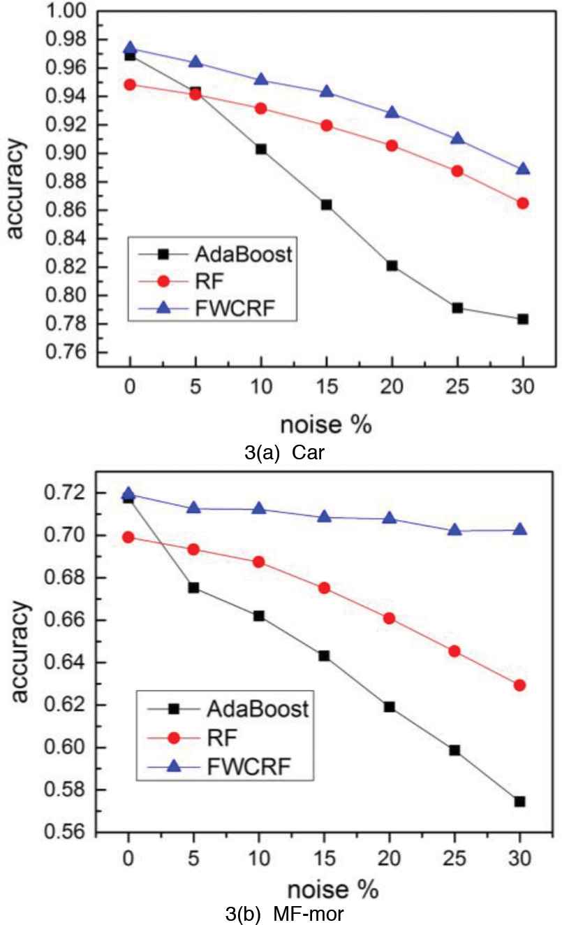
For the classification problem, the noise existing in the prediction features of training data is called input noise, and the noise existing on the class label is called output noise. In Breiman [5], the author points out that RF is more robust than AdaBoost on data with output noise. FWCRF not only uses the classic framework of RF, but also combines the multiple features at each split. Therefore, we infer that FWCRF should has better anti-noise ability than the classic RF and AdaBoost. In this paper, we implement the comparison of robustness on the datasets of categorical feature Car and numerical feature MF-mor.
In the experiments of output noise, we randomly add m% noise to samples in training set,

The Robustness of FWCRF compared with AdaBoost and random forest (RF) to output noise.
In the experiments of input noise, we add m% noise to the values of the prediction features,
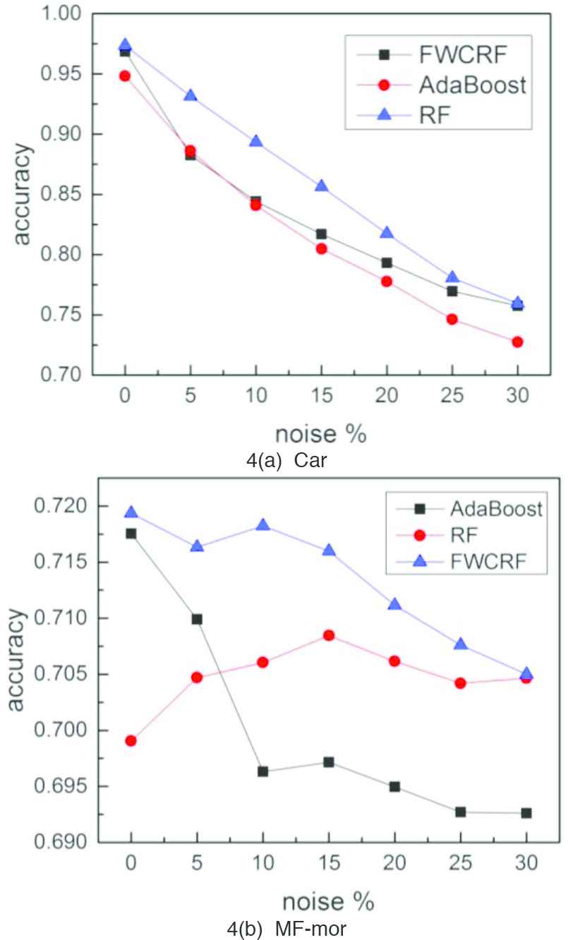
The Robustness of FWCRF compared with AdaBoost and random forest (RF) to iutput noise.
5. CONCLUSION
The RF [5] is known as a representative work of ensemble learning, which is suitable for high-dimensional data. However, it cannot get a good ensemble effect on low-dimensional data because the univariate split method cannot generate diverse individuals. Although the emergence of some oblique RFs based on numerical features partially solves the above problems, they cannot be directly applied to the datasets containing categorical features.
In this paper, we propose a feature-weighting and clustering method combining multiple variables. When splitting nodes, we first use Relief-F algorithm to weight features, and then use clustering algorithm based on weighted distance to split nodes. This method can be regarded as a variation of classical K-means. By defining the “center” and “distance between two points,” we make this method applicable to the categorical features. We use the DTs generated by this method as the base classifiers, and construct the ensemble classifier (FWCRF) based on the framework of RF. Finally, we compare FWCRF with the classical RF and AdaBoost on 31 datasets. The experimental results show that the FWCRF outperforms the other two ensembles on low-dimensional datasets, whose performance is comparable with the other two on the rest datasets. At the same time, we also verify that the robustness of FWCRF is superior to AdaBoost on the data with output noise.
CONFLICT OF INTEREST
The authors declare that they have no competing interests.
AUTHORS' CONTRIBUTIONS
The study was conceived and designed by Zhenyu Liu and Tao Wen and experiments performed by Wei Sun and Qilong Zhang. All authors read and approved the manuscript.
ACKNOWLEDGMENTS
The authors wish to thank the anonymous referees for their valuable comments and suggestions, which improved the technical content and the presentation of the paper. This work is supported by the National Nature Science Foundation of China under Grant 61772101, 61602075 and Key Natural Guidance Plan of Liaoning Province in 2018.
REFERENCES
Cite this article
TY  - JOUR
AU  - Zhenyu Liu
AU  - Tao Wen
AU  - Wei Sun
AU  - Qilong Zhang
PY  - 2020
DA  - 2020/12/07
TI  - Feature-Weighting and Clustering Random Forest
JO  - International Journal of Computational Intelligence Systems
SP  - 257
EP  - 265
VL  - 14
IS  - 1
SN  - 1875-6883
UR  - https://doi.org/10.2991/ijcis.d.201202.001
DO  - 10.2991/ijcis.d.201202.001
ID  - Liu2020
ER  -